Phase Transition of the Ising Model on Fractal Lattice

Abstract

Phase transition of the Ising model is investigated on a planar lattice that has a fractal structure. On the lattice, the number of bonds that cross the border of a finite area is doubled when the linear size of the area is extended by a factor of four. The free energy and the spontaneous magnetization of the system are obtained by means of the higher-order tensor renormalization group method. The system exhibits the order-disorder phase transition, where the critical indices are different from that of the square-lattice Ising model. An exponential decay is observed in the density matrix spectrum even at the critical point. It is possible to interpret that the system is less entangled because of the fractal geometry.

I Introduction

Phase transition and critical phenomena have been one of the central issues in statistical analyses of condensed matter physics Domb_Green . When the second-order phase transition is observed, thermodynamic functions, such as the free energy, the internal energy, and the magnetization, show non-trivial behavior around the transition temperature $T_{\rm c}^{~{}}$ Fisher ; Stanley . This critical singularity reflects the absence of any scale length at $T_{\rm c}^{~{}}$, and the power-law behavior of thermodynamic functions around the transition is explained by the concept of the renormalization group Kadanoff ; Kadanoff2 ; Wilson-Kogut ; Domb_Green .

Analytic investigation of the renormalization group flow in $\varphi^{4}_{~{}}$-model shows that the Ising model exhibits a phase transition when the lattice dimension is larger than one, which is the lower critical dimension Wilson-Kogut ; Justin . In a certain sense, the one-dimensional Ising model shows rescaled critical phenomena around $T_{\rm c}^{~{}}=0$. When the lattice dimension is larger than four, which is the upper critical dimension, and provided that the system is uniform, then the Ising model on regular lattices exhibits mean-field-like critical behavior.

Compared with critical phenomena on regular lattices, much less is known on fractal lattices. Renormalization flow is investigated by Gefen et al., Gefen1 ; Gefen2 ; Gefen3 ; Gefen4 where correspondence between lattice structure and the value of critical indices is not fully understood in a quantitative manner. For example, the Ising model on the Sierpinski gasket does not exhibit phase transition at any finite temperature, although the Hausdorff dimension of the lattice, $d_{\rm H}^{~{}}=\ln 3/\ln 2\approx 1.585$, is larger than one Gefen5 ; Luscombe . The absence of the phase transition could be explained by the fact that the number of interfaces, i.e. the outgoing bonds from a finite area, does not increase when the size of the area is doubled on the gasket. A non-trivial feature of this system is that there is a logarithmic scaling behavior in the internal energy toward zero temperature log . The effect of anisotropy has been considered recently Ran . In case of the Ising model on the Sierpinski carpet, presence of the phase transition is proved Vezzani , and its critical indices were roughly estimated by Monte Carlo simulations Carmona . It should be noted that it is not easy to collect sufficient number of data plots for finite-size scaling FSS on such fractal lattices by means of Monte Carlo simulations, because of the exponential blow-up of the number of sites in a unit of fractal.

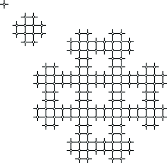
Figure 1: Composition of the fractal lattice. Upper left: a local vertex around an Ising spin shown by the empty dot. Middle: the basic cluster which contains $N_{1}^{~{}}=12$ vertices. Lower right: the extended cluster which contains $N_{2}^{~{}}=12^{2}_{~{}}$ vertices. In each step of the system extension, the linear size of the system increases by the factor of 4, where only 12 units are linked, and where 4 units at the corners are missing, if it is compared with a 4 by 4 square cluster.

In this article, we investigate the Ising model on a planar fractal lattice, shown in Fig. 1. The lattice consists of vertices around the lattice points, which are denoted by the empty dots in the figure, where there are Ising spins. The whole lattice is constructed by recursive extension processes, where the linear size of the system increases by the factor of four in each step. If the lattice was a regular square one, $4\times 4=16$ units are connected in the extension process, whereas only 12 units are connected on this fractal lattice; 4 units are missing in the corners. As a result, the number of sites contained in a cluster after $n$ extensions is $N_{n}^{~{}}=12^{n}_{~{}}$, and the Hausdorff dimension of this lattice is $d_{\rm H}^{~{}}=\ln 12/\ln 4\approx 1.792$. The number of outgoing bonds from a cluster is only doubled in each extension process since the sites and the bonds at each corner are missing. If we evaluate the lattice dimension from the relation

$$M=L^{d-1}_{~{}}$$ (1)

between the linear dimension $L$ and the number of outgoing bonds $M$, we have $d=1.5$, since $M$ is proportional to $\sqrt{L}$ on the fractal. Remark that the value is different from $d_{\rm H}^{~{}}\approx 1.792$

We report the critical behavior of the Ising model on the fractal lattice when the system size is large enough. Thermodynamic properties of the system are numerically studied by means of the Higher-Order Tensor Renormalization Group (HOTRG) method HOTRG . The system exhibits the order-disorder phase transition, where the critical indices are different from the square lattice Ising model. In the next Section we introduce a representation of the Ising model in terms of a vertex model, which is suitable for numerical analyses by means of the HOTRG method. In Sec. III, we show the calculated result around the transition temperature $T_{\rm c}^{~{}}$. Conclusions are summarized in the last Section.

II Vertex representation

We introduce a representation of the Ising model as a (symmetric) 16-vertex model. The Ising interaction between two adjacent Ising spins $\sigma$ and $\sigma^{\prime}$, where each one takes either $+1$ or $-1$, is represented by the diagonal Hamiltonian

$$H(\sigma,\sigma^{\prime})=-J\sigma\sigma^{\prime}\,,$$ (2)

where $J>0$ represents the ferromagnetic coupling. Throughout this article we assume that there is no external magnetic field. The corresponding local Boltzmann weight on the bond is given by

$$\exp\left[-\frac{H(\sigma,\sigma^{\prime})}{k_{\rm B}T}\right]=\exp\left[\frac{J}{k_{\rm B}T}\,\sigma\sigma^{\prime}\right]=e^{K\sigma\sigma^{\prime}}_{~{}}\,,$$ (3)

where $T$ is the temperature, $k_{\rm B}$ is the Boltzmann constant, and we have introduced a parameter $K=J/k_{\rm B}T$.

It is possible to factorize the bond weight $e^{K\sigma\sigma^{\prime}}_{~{}}$ into two parts, by introducing an auxiliary spin $s=\pm 1$, which is often called an ‘ancilla’, and which is located between $\sigma$ and $\sigma^{\prime}$ Fisher_M . A key relation is

$$e^{K\sigma\sigma^{\prime}}_{~{}}=\frac{1}{2\left(\cosh 2{\overline{K}}\right)^{1/2}_{~{}}}\,\sum_{s}^{~{}}\,e^{{\overline{K}}s(\sigma+\sigma^{\prime})}_{~{}}\,,$$ (4)

where the r.h.s. takes the value $\left(\cosh 2{\overline{K}}\right)^{1/2}_{~{}}$ when $\sigma=\sigma^{\prime}$, and $\left(\cosh 2{\overline{K}}\right)^{-1/2}_{~{}}$ when $\sigma\neq\sigma^{\prime}$, and where Eq. (4) holds under the condition

$$e^{K}_{~{}}=\left(\cosh 2{\overline{K}}\right)^{1/2}_{~{}}\,.$$ (5)

The new parameter ${\overline{K}}$ is then expressed as follows

$$e^{\overline{K}}_{~{}}=\sqrt{e^{2K}_{~{}}+\sqrt{e^{4K}_{~{}}-1}}\,.$$ (6)

Thus, if we introduce a factor

$$W_{\sigma s}^{~{}}=e^{\overline{K}\sigma s}_{~{}}\left[2\left(\cosh 2{\overline{K}}\right)^{1/2}_{~{}}\right]^{-1/2}_{~{}}$$ (7)

for each division of a bond, we can rewrite the Ising interaction in the following form

$$e^{K\sigma\sigma^{\prime}}_{~{}}=\sum_{s}^{~{}}\,W_{\sigma s}^{~{}}\,W_{\sigma^{\prime}s}^{~{}}\,.$$ (8)

By means of the factorization in Eq. (8), we can map the square-lattice Ising model into the symmetric 16-vertex model, where the local vertex weight is defined as

$$T_{s\,s^{\prime}s^{\prime\prime}s^{\prime\prime\prime}}^{~{}}=\sum_{\sigma}^{~{}}\,W_{\sigma s}^{~{}}\,W_{\sigma s^{\prime}}^{~{}}\,W_{\sigma s^{\prime\prime}}^{~{}}\,W_{\sigma s^{\prime\prime\prime}}^{~{}}\,.$$ (9)

In the upper-left corner of Fig. 1, we have shown the graphical representation of the vertex weight $T_{s\,s^{\prime}s^{\prime\prime}s^{\prime\prime\prime}}^{~{}}$, where the open circle denotes the Ising spin $\sigma$, which is summed up. The four short bars around the Ising spin in Fig. 1 show the halves of the bonds, where there are auxiliary spins $s$, $s^{\prime}$, $s^{\prime\prime}$, and $s^{\prime\prime\prime}$ at the end of each short bar.

In case we consider a finite-size cluster with rectangular shape with free boundary conditions, we have to prepare a new boundary Boltzmann weight

$$P_{s\,s^{\prime}s^{\prime\prime}}^{~{}}=\sum_{\sigma}^{~{}}\,W_{\sigma s}^{~{}}\,W_{\sigma s^{\prime}}^{~{}}\,W_{\sigma s^{\prime\prime}}^{~{}}$$ (10)

and a corner Boltzmann weight

$$C_{s\,s^{\prime}}^{~{}}=\sum_{\sigma}^{~{}}\,W_{\sigma s}^{~{}}\,W_{\sigma s^{\prime}}^{~{}}\,.$$ (11)

It should be noted that these boundary weights $P_{s\,s^{\prime}s^{\prime\prime}}^{~{}}$ and $C_{s\,s^{\prime}}^{~{}}$ are obtained by taking partial trace for the vertex weight; we have the relations

$$P_{s\,s^{\prime}s^{\prime\prime}}^{~{}}=\frac{\sum_{s^{\prime\prime\prime}}^{~{}}\,T_{s\,s^{\prime}s^{\prime\prime}s^{\prime\prime\prime}}^{~{}}}{\sum_{s^{\prime\prime\prime}}^{~{}}\,W_{\sigma s^{\prime\prime\prime}}^{~{}}}$$ (12)

and

$$C_{s\,s^{\prime}}^{~{}}=\frac{\sum_{s^{\prime\prime}s^{\prime\prime\prime}}^{~{}}T_{s\,s^{\prime}s^{\prime\prime}s^{\prime\prime\prime}}^{~{}}}{(\sum_{s^{\prime\prime}}^{~{}}\,W_{\sigma s^{\prime\prime}}^{~{}})(\sum_{s^{\prime\prime\prime}}^{~{}}\,W_{\sigma s^{\prime\prime\prime}}^{~{}})}\,,$$ (13)

where one can neglect the denominator when one is interested in the critical singularity; the denominators just subtract a regular function from the free energy of the system. In case that one needs fixed boundary conditions, it is sufficient to avoid taking the configuration sum for $\sigma$ in the r.h.s. of both Eq. (10) and Eq. (11), and to set all the boundary spins to be either $+1$ or $-1$ according to the condition. The vertex weights $T_{s\,s^{\prime}s^{\prime\prime}s^{\prime\prime\prime}}^{~{}}$, $P_{s\,s^{\prime}s^{\prime\prime}}^{~{}}$, and $C_{s\,s^{\prime}}^{~{}}$ are invariant under arbitrary permutation of the indices.

There are various choices of the factorization of the bond weight in Eq. (8). Instead of using the relation in Eq. (7), one can introduce an asymmetric decomposition

$$W=\left(\begin{array}[]{cc}\sqrt{\cosh K},&\sqrt{\sinh K}\\ \sqrt{\cosh K},&-\sqrt{\sinh K}\end{array}\right)\,,$$ (14)

where we have used the matrix notation for the weight $W_{\sigma s}^{~{}}$. This expression is often employed in the tensor network formulations HOTRG , which does not require any typical symmetry for local weights, as long as the numerical treatment is concerned. In case this asymmetric factorization in Eq. (14) is employed, one has to care about the order of the indices in $T_{s\,s^{\prime}s^{\prime\prime}s^{\prime\prime\prime}}^{~{}}$ RG . In the following numerical calculation, we use the symmetric factorization.

The fractal lattice we treat in this article is constructed by a recursive joining process of the local tensors, which is nothing but a vertex weight in Eq. (9) at the beginning. In each extension process, we join 12 local tensors as shown in the middle of Fig. 1. In the joining process, we take the configuration sum for those tensor indices inside the cluster, leaving those on the border that become new tensor indices of the extended tensor. Because of the fractal geometry, some of the bonds inside the cluster are not connected with each other. We also take configuration sum for these dangling bonds, and the process just change the normalization of the partition function by amount of

$$\sum_{s}^{~{}}\,W_{\sigma s}^{~{}}=2\cosh{\overline{K}}\,\left[2\left(\cosh 2{\overline{K}}\right)^{1/2}_{~{}}\right]^{-1/2}_{~{}}$$ (15)

for each, if we choose the definition of $W_{\sigma s}^{~{}}$ in Eq. (7). We take the rescaling effect into account, although the rescaling is not essential to the thermodynamic properties of the system, in particular to its critical singularity. In this manner, what we are dealing with is the Ising model, where there are only spins denoted by the empty dots in Fig. 1.

At first we have only 4 spins $s$, $s^{\prime}$, $s^{\prime\prime}$, and $s^{\prime\prime\prime}$ on the outgoing bonds, and after $n$ extensions of the system, we have $4\times 2^{n}_{~{}}$ border spins on the surface of the extended cluster. The application of the HOTRG to this fractal system is straightforward. The recursive structure of the lattice is suitable for the repeated process of system extensions and renormalization group transformations in the HOTRG method. The partition function $Z_{n}^{~{}}(T)$ of the system after $n$ extensions is obtained by the contraction of the extended tensors; we choose the periodic boundary conditions to evaluate

$$Z_{n}^{~{}}(T)=\sum_{ij}^{~{}}\,T_{ijij}^{(n)}\,,$$ (16)

where $T_{ijkl}^{(n)}$ is the renormalized local tensor obtained after $n$ extensions.

III Numerical Results

In order to simplify the numerical analysis, we choose the parameterization $J=k_{\rm B}=1$, and thus we have $K=1/T$. In the numerical calculation by means of HOTRG, we keep $D=24$ states at most for block spin variables. We have verified that the choice $D=24$ is sufficient for obtaining the converged free energy

$$F_{n}^{~{}}(T)=-k_{\rm B}T\ln Z_{n}^{~{}}(T)$$ (17)

in the entire temperature region chi . We treat the free energy per site

$$f(T)=\lim_{n\rightarrow\infty}^{~{}}\,\frac{F_{n}^{~{}}(T)}{N_{n}^{~{}}}$$ (18)

in the following thermodynamic analyses, where the r.h.s. converges already for $n\lesssim 30$ .

Figure 2 shows the temperature dependence of the specific heat per site

$$c(T)=\frac{\partial}{\partial T}\,u(T)\,,$$ (19)

where $u(T)$ is the internal energy per site

$$u(T)=-T^{2}_{~{}}\,\frac{\partial}{\partial T}\,\frac{f(T)}{T}\,,$$ (20)

and the temperature derivatives are performed numerically. There is no singularity in $c(T)$ around its maximum. One might find a weak non-analytic behavior at $T_{\rm c}^{~{}}\approx 1.317$, which is marked by the dotted line in the figure; the numerical derivative of $c(T)$ with respect to temperature (plotted in the inset) has a sharp peak at the critical temperature $T_{\rm c}^{~{}}$. It is, however, difficult to determine the critical exponent $\alpha$ precisely, because of the weakness in the singularity; as shown in the figure, $c(T)$ around $T_{\rm c}^{~{}}$ is almost linear in $T$, and therefore $\alpha$ is nearly zero.

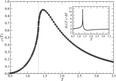
Figure 2: The specific heat $c(T)$ per site in Eq. (19). Inset: numerical derivative of $c(T)$ with respect to temperature; a sharp peak is observed at $T_{\rm c}^{~{}}\approx 1.317$.

Figure 3 shows the spontaneous magnetization per site $m(T)$, which is obtained by inserting a $\sigma$-dependent local weight

$${\tilde{T}}_{s\,s^{\prime}s^{\prime\prime}s^{\prime\prime\prime}}^{~{}}=\sum_{\sigma}^{~{}}\,\sigma\,W_{\sigma s}^{~{}}\,W_{\sigma s^{\prime}}^{~{}}\,W_{\sigma s^{\prime\prime}}^{~{}}\,W_{\sigma s^{\prime\prime\prime}}^{~{}}$$ (21)

into the system. Since the fractal lattice is inhomogeneous, the value is weakly dependent on the location of the observation site, but the critical behavior is not affected by the location; we choose a site from the four sites that are in the middle of the 12-site cluster shown in Fig. 1. The numerical calculation by HOTRG captures the spontaneous magnetization $m(T)$ below $T_{\rm c}^{~{}}$ since any tiny round-off error is sufficient for breaking the symmetry inside low-temperature ordered state. Around the transition temperature, the magnetization satisfies a power-law behavior

$$m(T)\propto|T_{\rm c}^{~{}}-T|^{0.0137}_{~{}}\,,$$ (22)

where the precision of the exponent is around 2%, which can be read out from the inset of Fig. 3 as a tiny deviation from the linear dependence (the dashed lines) in $m(T)^{1/\beta}$ near $T_{\rm c}^{~{}}$.

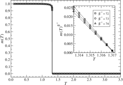
Figure 3: The spontaneous magnetization per site $m(T)$. Inset: the power-law behavior below $T_{\rm c}^{~{}}=1.31716$.

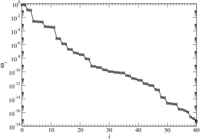
Figure 4: Decay of the singular values after $n=8$ extensions.

As a byproduct of the numerical HOTRG calculation, we can roughly observe the entanglement spectrum, entanglement which is the distribution of the eigenvalue $\omega_{i}^{~{}}$ of the density matrix that is created for the purpose of obtaining the block spin transformation. Since the effect of environment is not considered in our implementation of the HOTRG method, the eigenvalue $\omega_{i}^{~{}}=\lambda^{2}_{i}$ is obtained as the square of the singular values $\lambda_{i}^{~{}}$ in the higher-order singular value decomposition applied to the extended tensors. Figure 4 shows $\omega_{i}^{~{}}$ at $T=T_{\rm c}^{~{}}$ in the decreasing order. The decay is rapid, and therefore further increase of the number of block-spin state from $D=24$ to a larger number does not significantly improve the precision in $Z_{n}^{~{}}$; the difference in $f(T_{\rm c}^{~{}})$ between $D=8$ and $D=16$ is already of the order of $10^{-6}_{~{}}$. It should be noted that the eigenvalues are not distributed equidistantly in logarithmic scale; the corner double line structure is absent CDL1 ; CDL2 .

IV Conclusions and Discussions

We have investigated the Ising model on the fractal lattice shown in Fig. 1 by means of the HOTRG method. The calculated specific heat $c(T)$ suggests that the model shows 2^nd order phase transition. Qualitatively speaking, the presence of weak singularity in the specific heat agrees with the result of the $\epsilon$-expansion, which shows the increasing nature of the critical exponent in $c(T)$ with respect to the space dimension $d~{}$ Wilson-Kogut . The calculated spontaneous magnetization $m(T)$ also supports the 2^nd order phase transition with the exponent $\beta_{\rm fractal}^{~{}}\approx 0.0137$, which is smaller by one order of magnitude than the critical exponent $\beta_{\rm square}^{~{}}=1/8=0.125$ of the square-lattice Ising model.

The fractal structure of the lattice modifies the entanglement spectrum from that on the square lattice explained by the corner double line picture CDL1 ; CDL2 . Since each corner is missing in the fractal structure in Fig. 1, short-range entanglement is almost filtered out in the process of the renormalization group transformation. This may be the reason why we do not need many degrees of freedom for the renormalized tensors. The situation is similar to the entanglement structure reported in the tensor network renormalization TNR1 ; TNR2 ; TNR3 ; TNR4 ; TNR5 ; Loop .

The lattice geometry of the fractal lattice can be modified in several manners. For example, one can alternate the system extension process of the fractal for the purpose of modifying the Hausdorff dimension; for every odd $n$ the extension with 12 vertices shown in Fig. 1 is performed, and for even $n$ the normal extension with 16 vertices on the square-lattice is performed. Alternatively, one can also modify the basic cluster, in such a manner as introducing 6 by 6 cluster where 4 corners are missing, etc. It is also worth considering three-dimensional fractal lattice, and apply the HOTRG method as it was done for the cubic lattice Ising model Xie . These modifications do not spoil the applicability of the HOTRG method while the numerical requirement is heavier than the current research. Analyses of quantum systems on a variety of fractal lattice is another possible extensions Voigt1 ; Voigt2 . These further study may clarify the role of the entanglement in the universality of the phase transition in both regular and fractal lattices.

- (1) Phase transitions and critical phenomena, vol. 1-20, ed. C. Domb, M.S. Green, and J. Lebowitz (Academic Press, 1972-2001).
- (2) H.E. Stanley, Introduction to Phase Transitions and Critical Phenomena, (Oxford, 1971).
- (3) M.E. Fisher, Rev. Mod. Phys. 46, 597 (1974) and references therein.
- (4) L.P. Kadanoff, Physics 2, 263 (1966).
- (5) E. Efrati, Z. Wang, A. Kolan, and L.P. Kadanoff, Rev. Mod. Phys. 86 647 (2014).
- (6) K.G. Wilson and J. Kogut, Phys. Rep. 12, 75 (1974).
- (7) J. Zinn-Justin, Quantum Field Theory and Critical Phenomena, (Oxford, 1996).
- (8) Y. Gefen, B.B. Mandelbrot, and A. Aharony, Phys. Rev. Lett. 45, 855-858 (1980).
- (9) Y. Gefen, Y. Meir, B.B. Mandelbrot, and A. Aharony, Phys. Rev. Lett. 50, 145-148 (1983).
- (10) Y. Gefen, A. Aharony, and B.B. Mandelbrot, J. Phys. A: Math. Gen. 16, 1267-1278 (1983).
- (11) Y. Gefen, A. Aharony, and B.B. Mandelbrot , J. Phys. A: Math. Gen. 17, 1277-1289 (1984).
- (12) Y. Gefen, A. Aharony, Y. Shapir, and B.B. Mandelbrot, J. Phys. A 17, 435 (1984).
- (13) J.H. Luscombe and R.C. Desai, Phys. Rev. B 32, 1614 (1985).
- (14) T. Stošić, B.D. Stošić, S. Milošević, and H.E. Stanley, Physica A 233, 31 (1996).
- (15) M. Wang, S.J. Ran, T. Liu, Y. Zhao, Q.R. Zheng and G. Su, to appear in Euro. Phys. J. B; arXiv:1311.1502.
- (16) A. Vezzani, J. Phys. A: Mathe. Gen. 36, 1593 (2003).
- (17) J.M. Carmona, Umberto Marini Bettolo Marconi, J.J. Ruiz-Lorenzo, A. Tarancon, Phys. Rev. B 58, 14387 (1998).
- (18) T.W. Burkhardt and J.M.J. van Leeuwen, Real-space renormalization, Topics in Current Physics 30 (Springer, Berlin, 1982), and references therein.
- (19) Z.Y. Xie, J. Chen, M.P. Qin, J.W. Zhu, L.P. Yang, T. Xiang, Phys. Rev. B 86, 045139 (2012).
- (20) M.E. Fisher, Proc. Roy. Soc. A 254, 66 (1960).
- (21) The symmetry in the local tensors is not always preserved when one performs the renormalization group transformation in the HOTRG method. Thus, for most of the cases, the symmetry is not that important in the numerical calculations.
- (22) A larger value of is necessary if one needs tiny density-matrix eigenvalues for the purpose of analyzing their asymptotic decay.
- (23) It is possible to identify the system boundary of a finite area of 2d classical lattice models as ‘a wave function’ of a certain 1d quantum system. In this manner one naturally finds the quantum-classical correspondence, and can introduce the notion of entanglement in classical lattice models.
- (24) Z.C. Gu and X.G. Wen, Phys. Rev. B 80, 155131 (2009).
- (25) H. Ueda, K. Okunishi, and T. Nishino, Phys. Rev. B 89, 075116 (2014).
- (26) G. Evenbly and G. Vidal, Phys. Rev. Lett. 115, 180405 (2015).
- (27) G. Evenbly and G. Vidal, Phys. Rev. Lett. 115, 200401 (2015).
- (28) G. Evenbly, arXiv: 1509.07484.
- (29) G. Evenbly and G. Vidal, arXiv: 1510.00689.
- (30) M. Hauru, G. Evenbly, W.W. Ho, D. Gaiotto, and G. Vidal, arXiv: 1512.03846.
- (31) S. Yang, Z.C. Gu, and X.G. Wen, arXiv: 1512.04938.
- (32) Z.Y. Xie, J. Chen, M.P. Qin, J.W. Zhu, L.P. Yang, and T Xiang, Phys. Rev. B 86, 045139 (2012).
- (33) A. Voigt, J. Richter, P. Tomczak, and Physica A 299, 461 (2001).
- (34) A. Voigt, W. Wenzel, J. Richter, and P. Tomczak, Eur. Phys. J. B 38, 49 (2004).