TransG : A Generative Model for Knowledge Graph Embedding

TransG : A Generative Model for Knowledge Graph Embedding

Abstract

Recently, knowledge graph embedding, which projects symbolic entities and relations into continuous vector space, has become a new, hot topic in artificial intelligence. This paper proposes a novel generative model (TransG) to address the issue of multiple relation semantics that a relation may have multiple meanings revealed by the entity pairs associated with the corresponding triples. The new model can discover latent semantics for a relation and leverage a mixture of relation-specific component vectors to embed a fact triple. To the best of our knowledge, this is the first generative model for knowledge graph embedding, and at the first time, the issue of multiple relation semantics is formally discussed. Extensive experiments show that the proposed model achieves substantial improvements against the state-of-the-art baselines. All of the related poster, slides, datasets and codes have been published in http://www.ibookman.net/conference.html.

1 Introduction

Abstract or real-world knowledge is always a major topic in Artificial Intelligence. Knowledge bases such as Wordnet [Miller, 1995] and Freebase [Bollacker et al., 2008] have been shown very useful to AI tasks including question answering, knowledge inference, and so on. However, traditional knowledge bases are symbolic and logic, thus numerical machine learning methods cannot be leveraged to support the computation over the knowledge bases. To this end, knowledge graph embedding has been proposed to project entities and relations into continuous vector spaces. Among various embedding models, there is a line of translation-based models such as TransE [Bordes et al., 2013], TransH [Wang et al., 2014], TransR [Lin et al., 2015b], and other related models [He et al., 2015] [Lin et al., 2015a].

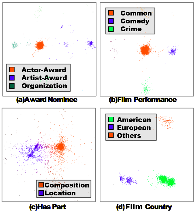
Figure 1: Visualization of TransE embedding vectors with PCA dimension reduction. Four relations (a $\thicksim$ d) are chosen from Freebase and Wordnet. A dot denotes a triple and its position is decided by the difference vector between tail and head entity ($\mathbf{t-h}$). Since TransE adopts the principle of $\mathbf{t-h\approx r}$, there is supposed to be only one cluster whose centre is the relation vector $\mathbf{r}$. However, results show that there exist multiple clusters, which justifies our multiple relation semantics assumption.

A fact of knowledge base can usually be represented by a triple $(h,r,t)$ where $h,r,t$ indicate a head entity, a relation, and a tail entity, respectively. All translation-based models almost follow the same principle $\mathbf{h_{r}+r\approx t_{r}}$ where $\mathbf{h_{r},r,t_{r}}$ indicate the embedding vectors of triple $(h,r,t)$, with the head and tail entity vector projected with respect to the relation space.

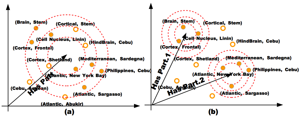
Figure 2: Visualization of multiple relation semantics. The data are selected from Wordnet. The dots are correct triples that belong to $\mathrm{HasPart}$ relation, while the circles are incorrect ones. The point coordinate is the difference vector between tail and head entity, which should be near to the centre. (a) The correct triples are hard to be distinguished from the incorrect ones. (b) By applying multiple semantic components, our proposed model could discriminate the correct triples from the wrong ones.

In spite of the success of these models, none of the previous models has formally discussed the issue of multiple relation semantics that a relation may have multiple meanings revealed by the entity pairs associated with the corresponding triples. As can be seen from Fig. 1, visualization results on embedding vectors obtained from TransE [Bordes et al., 2013] show that, there are different clusters for a specific relation, and different clusters indicate different latent semantics. For example, the relation HasPart has at least two latent semantics: composition-related as (Table, HasPart, Leg) and location-related as (Atlantics, HasPart, NewYorkBay). As one more example, in Freebase, (Jon Snow, birth place, Winter Fall) and (George R. R. Martin, birth place, U.S.) are mapped to schema /fictional_universe/fictional_character/place_of_birth and /people/person/place_of_birth respectively, indicating that birth place has different meanings. This phenomenon is quite common in knowledge bases for two reasons: artificial simplification and nature of knowledge. On one hand, knowledge base curators could not involve too many similar relations, so abstracting multiple similar relations into one specific relation is a common trick. On the other hand, both language and knowledge representations often involve ambiguous information. The ambiguity of knowledge means a semantic mixture. For example, when we mention “Expert”, we may refer to scientist, businessman or writer, so the concept “Expert” may be ambiguous in a specific situation, or generally a semantic mixture of these cases.

However, since previous translation-based models adopt $\mathbf{h_{r}+r\approx t_{r}}$, they assign only one translation vector for one relation, and these models are not able to deal with the issue of multiple relation semantics. To illustrate more clearly, as showed in Fig.2, there is only one unique representation for relation $\mathrm{HasPart}$ in traditional models, thus the models made more errors when embedding the triples of the relation. Instead, in our proposed model, we leverage a Bayesian non-parametric infinite mixture model to handle multiple relation semantics by generating multiple translation components for a relation. Thus, different semantics are characterized by different components in our embedding model. For example, we can distinguish the two clusters $\mathrm{HasPart.1}$ or $\mathrm{HasPart.2}$, where the relation semantics are automatically clustered to represent the meaning of associated entity pairs.

To summarize, our contributions are as follows:

• We propose a new issue in knowledge graph embedding, multiple relation semantics that a relation in knowledge graph may have different meanings revealed by the associated entity pairs, which has never been studied previously.

• To address the above issue, we propose a novel Bayesian non-parametric infinite mixture embedding model, TransG. The model can automatically discover semantic clusters of a relation, and leverage a mixture of multiple relation components for translating an entity pair. Moreover, we present new insights from the generative perspective.

• Extensive experiments show that our proposed model obtains substantial improvements against the state-of-the-art baselines.

2 Related Work

Prior studies are classified into two branches: translation-based embedding methods and the others.

2.1 Translation-Based Embedding Methods

Existing translation-based embedding methods share the same translation principle $\mathbf{h+r\approx t}$ and the score function is designed as:

$$f_{r}(h,t)=||\mathbf{h_{r}+r-t_{r}}||_{2}^{2}$$

where $\mathbf{h_{r},t_{r}}$ are entity embedding vectors projected in the relation-specific space. TransE [Bordes et al., 2013], lays the entities in the original entity space: $\mathbf{h_{r}=h,t_{r}=t}$. TransH [Wang et al., 2014], projects entities into a hyperplane for addressing the issue of complex relation embedding: $\mathbf{h_{r}=h-w_{r}^{\top}hw_{r},t_{r}=t-w_{r}^{\top}tw_{r}}$. To address the same issue, TransR [Lin et al., 2015b], transforms the entity embeddings by the same relation-specific matrix: $\mathbf{h_{r}=M_{r}h,t_{r}=M_{r}t}$. TransR also proposes an ad-hoc clustering-based method, CTransR, where the entity pairs for a relation are clustered into different groups, and the pairs in the same group share the same relation vector. In comparison, our model is more elegant to address such an issue theoretically, and does not require a pre-process of clustering. Furthermore, our model has much better performance than CTransR, as we expect. TransM [Fan et al., 2014] leverages the structure of the knowledge graph via pre-calculating the distinct weight for each training triple to enhance embedding. KG2E [He et al., 2015] is a probabilistic embedding method for modeling the uncertainty in knowledge graph.

2.2 Pioneering Embedding Methods

There list the pioneering embedding approaches:

Structured Embedding (SE). The SE model [Bordes et al., 2011] transforms the entity space with the head-specific and tail-specific matrices. The score function is defined as $f_{r}(h,t)=||\mathbf{M_{h,r}h-M_{t,r}t}||$. According to [Socher et al., 2013], this model cannot capture the relationship between entities. Semantic Matching Energy (SME). The SME model [Bordes et al., 2012] [Bordes et al., 2014] can handle the correlations between entities and relations by matrix product and Hadamard product. In some recent work [Bordes et al., 2014], the score function is re-defined with 3-way tensors instead of matrices. Single Layer Model (SLM). SLM applies neural network to knowledge graph embedding. The score function is defined as $f_{r}(h,t)=\mathbf{u_{r}^{\top}}g(\mathbf{M_{r,1}h+M_{r,2}t})$ where $\mathbf{M_{r,1},M_{r,2}}$ are relation-specific weight matrices. Collobert had applied a similar method into the language model, [Collobert and Weston, 2008]. Latent Factor Model (LFM). The LFM [Jenatton et al., 2012], [Sutskever et al., 2009] attempts to capture the second-order correlations between entities by a quadratic form. The score function is as $f_{r}(h,t)=\mathbf{h^{\top}W_{r}t}$. Neural Tensor Network (NTN). The NTN model [Socher et al., 2013] defines a very expressive score function to combine the SLM and LFM: $f_{r}(h,t)=\mathbf{u_{r}^{\top}}g(\mathbf{h^{\top}W_{\cdot\cdot r}t+M_{r,1}h+M_{r,2}t+b_{r}})$, where $\mathbf{u_{r}}$ is a relation-specific linear layer, $g(\cdot)$ is the $tanh$ function, $\mathbf{W}\in\mathbb{R}^{d\times d\times k}$ is a 3-way tensor. Unstructured Model (UM). The UM [Bordes et al., 2012] may be a simplified version of TransE without considering any relation-related information. The score function is directly defined as $f_{r}(h,t)=||\mathbf{h-t}||_{2}^{2}$. RESCAL. This is a collective matrix factorization model which is also a common method in knowledge base embedding [Nickel et al., 2011], [Nickel et al., 2012].

Semantically Smooth Embedding (SSE). [Guo et al., 2015] aims at further discovering the geometric structure of the embedding space to make it semantically smooth. [Wang et al., 2014] focuses on bridging the gap between knowledge and texts, with a joint loss function for knowledge graph and text corpus. [Wang et al., 2015] incorporates the rules that are related with relation types such as 1-N and N-1. PTransE. [Lin et al., 2015a] is a path-based embedding model, simultaneously considering the information and confidence level of the path in knowledge graph.

3 Methods

3.1 TransG: A Generative Model for Embedding

As just mentioned, only one single translation vector for a relation may be insufficient to model multiple relation semantics. In this paper, we propose to use Bayesian non-parametric infinite mixture embedding model [Griffiths and Ghahramani, 2011]. The generative process of the model is as follows:

1. For an entity $e\in E$:

   1. Draw each entity embedding mean vector from a standard normal distribution as a prior: $\mathbf{u_{e}\backsim\mathcal{N}(0,1)}$.

2. For a triple $(h,r,t)\in\Delta$:

   1. Draw a semantic component from Chinese Restaurant Process for this relation: $\pi_{r,m}\thicksim CRP(\beta)$.

   2. Draw a head entity embedding vector from a normal distribution: $\mathbf{h}\backsim\mathcal{N}(\mathbf{u_{h}},\sigma_{h}^{2}\mathbf{E})$.

   3. Draw a tail entity embedding vector from a normal distribution: $\mathbf{t}\backsim\mathcal{N}(\mathbf{u_{t}},\sigma_{t}^{2}\mathbf{E})$.

   4. Draw a relation embedding vector for this semantics: $\mathbf{u_{r,m}}=\mathbf{t-h}\backsim\mathcal{N}(\mathbf{u_{t}-u_{h}},(\sigma_{h}^{2}+\sigma_{t}^{2})\mathbf{E})$.

where $\mathbf{u_{h}}$ and $\mathbf{u_{t}}$ indicate the mean embedding vector for head and tail respectively, $\sigma_{h}$ and $\sigma_{t}$ indicate the variance of corresponding entity distribution respectively, and $\mathbf{u_{r,m}}$ is the $m$-th component translation vector of relation $r$. Chinese Restaurant Process (CRP) is a Dirichlet Process and it can automatically detect semantic components. In this setting, we obtain the score function as below:

$$\mathbb{P}\{(h,r,t)\} \propto\sum_{m=1}^{M_{r}}\pi_{r,m}\mathbb{P}(\mathbf{u_{r,m}}|h,t)$$ (1)

$$=\sum_{m=1}^{M_{r}}\pi_{r,m}e^{-\frac{||\mathbf{u_{h}+u_{r,m}-u_{t}}||_{2}^{2}}{\sigma_{h}^{2}+\sigma_{t}^{2}}}$$

where $\pi_{r,m}$ is the mixing factor, indicating the weight of $i$-th component and $M_{r}$ is the number of semantic components for the relation $r$, which is learned from the data automatically by the CRP.

Inspired by Fig.1, TransG leverages a mixture of relation component vectors for a specific relation. Each component represents a specific latent meaning. By this way, TransG could distinguish multiple relation semantics. Notably, the CRP could generate multiple semantic components when it is necessary and the relation semantic component number $M_{r}$ is learned adaptively from the data.

3.2 Explanation from the Geometry Perspective

Similar to previous studies, TransG has geometric explanations. In the previous methods, when the relation $r$ of triple $(h,r,t)$ is given, the geometric representations are fixed, as $\mathbf{h+r\approx t}$. However, TransG generalizes this geometric principle to:

$$m_{(h,r,t)}^{*}=\underset{m=1...M_{r}}{\arg\max}~{}~{}\left(\pi_{r,m}e^{-\frac{||\mathbf{u_{h}+u_{r,m}-u_{t}}||_{2}^{2}}{\sigma_{h}^{2}+\sigma_{t}^{2}}}\right)$$

$$\mathbf{h+u_{r,m_{(h,r,t)}^{*}}}\approx\mathbf{t}$$ (2)

where $m_{(h,r,t)}^{*}$ is the index of primary component. Though all the components contribute to the model, the primary one contributes the most due to the exponential effect ($exp(\cdot)$). When a triple $(h,r,t)$ is given, TransG works out the index of primary component then translates the head entity to the tail one with the primary translation vector.

For most triples, there should be only one component that have significant non-zero value as $\left(\pi_{r,m}e^{-\frac{||\mathbf{u_{h}+u_{r,m}-u_{t}}||_{2}^{2}}{\sigma_{h}^{2}+\sigma_{t}^{2}}}\right)$ and the others would be small enough, due to the exponential decay. This property reduces the noise from the other semantic components to better characterize multiple relation semantics. In detail, $\mathbf{\left(t-h\right)}$ is almost around only one translation vector $\mathbf{u_{r,m_{(h,r,t)}^{*}}}$ in TransG. Under the condition $m\neq m_{(h,r,t)}^{*}$, $\left(\mathbf{\frac{||\mathbf{u_{h}+u_{r,m}-u_{t}}||_{2}^{2}}{\sigma_{h}^{2}+\sigma_{t}^{2}}}\right)$ is very large so that the exponential function value is very small. This is why the primary component could represent the corresponding semantics.

Table 1: Statistics of datasets

Data	WN18	FB15K	WN11	FB13
#Rel	18	1,345	11	13
#Ent	40,943	14,951	38,696	75,043
#Train	141,442	483,142	112,581	316,232
#Valid	5,000	50,000	2,609	5,908
#Test	5,000	59,071	10,544	23,733

Table 2: Evaluation results on link prediction

Datasets	WN18				FB15K
Metric	Mean Rank		HITS@10(%)		Mean Rank		HITS@10(%)
	Raw	Filter	Raw	Filter	Raw	Filter	Raw	Filter
Unstructured [Bordes et al., 2011]	315	304	35.3	38.2	1,074	979	4.5	6.3
RESCAL [Nickel et al., 2012]	1,180	1,163	37.2	52.8	828	683	28.4	44.1
SE　[Bordes et al., 2011]	1,011	985	68.5	80.5	273	162	28.8	39.8
SME(bilinear) [Bordes et al., 2012]	526	509	54.7	61.3	284	158	31.3	41.3
LFM [Jenatton et al., 2012]	469	456	71.4	81.6	283	164	26.0	33.1
TransE [Bordes et al., 2013]	263	251	75.4	89.2	243	125	34.9	47.1
TransH [Wang et al., 2014]	401	388	73.0	82.3	212	87	45.7	64.4
TransR [Lin et al., 2015b]	238	225	79.8	92.0	198	77	48.2	68.7
CTransR [Lin et al., 2015b]	231	218	79.4	92.3	199	75	48.4	70.2
KG2E [He et al., 2015]	362	348	80.5	93.2	183	69	47.5	71.5
TransG (this paper)	483	470	81.4	93.3	203	98	52.8	79.8

To summarize, previous studies make translation identically for all the triples of the same relation, but TransG automatically selects the best translation vector according to the specific semantics of a triple. Therefore, TransG could focus on the specific semantic embedding to avoid much noise from the other unrelated semantic components and result in promising improvements than existing methods. Note that, all the components in TransG have their own contributions, but the primary one makes the most.

3.3 Training Algorithm

The maximum data likelihood principle is applied for training. As to the non-parametric part, $\pi_{r,m}$ is generated from the CRP with Gibbs Sampling, similar to [He et al., 2015] and [Griffiths and Ghahramani, 2011]. A new component is sampled for a triple (h,r,t) with the below probability:

$$\mathbb{P}(m_{r,new})=\frac{\beta e^{-\frac{||\mathbf{h-t}||_{2}^{2}}{\sigma_{h}^{2}+\sigma_{t}^{2}+2}}}{\beta e^{-\frac{||\mathbf{h-t}||_{2}^{2}}{\sigma_{h}^{2}+\sigma_{t}^{2}+2}}+\mathbb{P}\{(h,r,t)\}}$$ (3)

Table 3: Evaluation results on FB15K by mapping properties of relations(%)

Tasks	Predicting Head(HITS@10)				Predicting Tail(HITS@10)
Relation Category	1-1	1-N	N-1	N-N	1-1	1-N	N-1	N-N
Unstructured [Bordes et al., 2011]	34.5	2.5	6.1	6.6	34.3	4.2	1.9	6.6
SE　[Bordes et al., 2011]	35.6	62.6	17.2	37.5	34.9	14.6	68.3	41.3
SME(bilinear) [Bordes et al., 2012]	30.9	69.6	19.9	38.6	28.2	13.1	76.0	41.8
TransE [Bordes et al., 2013]	43.7	65.7	18.2	47.2	43.7	19.7	66.7	50.0
TransH [Wang et al., 2014]	66.8	87.6	28.7	64.5	65.5	39.8	83.3	67.2
TransR [Lin et al., 2015b]	78.8	89.2	34.1	69.2	79.2	37.4	90.4	72.1
CTransR [Lin et al., 2015b]	81.5	89.0	34.7	71.2	80.8	38.6	90.1	73.8
TransG (this paper)	85.4	95.7	44.7	80.8	84.0	56.5	95.0	83.3

where $\mathbb{P}\{(h,r,t)\}$ is the current posterior probability. As to other parts, in order to better distinguish the true triples from the false ones, we maximize the ratio of likelihood of the true triples to that of the false ones. Notably, the embedding vectors are initialized by [Glorot and Bengio, 2010]. Putting all the other constraints together, the final objective function is obtained, as follows:

$$\min_{\mathbf{u_{h},u_{r,m},u_{t}}}\mathcal{L}$$

$$\mathcal{L}=-\sum_{(h,r,t)\in\Delta}ln\left(\sum_{m=1}^{M_{r}}\pi_{r,m}e^{-\frac{||\mathbf{u_{h}+u_{r,m}-u_{t}}||_{2}^{2}}{\sigma_{h}^{2}+\sigma_{t}^{2}}}\right)$$

$$+\sum_{(h^{\prime},r^{\prime},t^{\prime})\in\Delta^{\prime}}ln\left(\sum_{m=1}^{M_{r}}\pi_{r^{\prime},m}e^{-\frac{||\mathbf{u_{h^{\prime}}+u_{r^{\prime},m}-u_{t^{\prime}}}||_{2}^{2}}{\sigma_{h^{\prime}}^{2}+\sigma_{t^{\prime}}^{2}}}\right)$$

$$+C\left(\sum_{r\in R}\sum_{m=1}^{M_{r}}||\mathbf{u_{r,m}}||_{2}^{2}+\sum_{e\in E}||\mathbf{u_{e}}||^{2}_{2}\right)$$ (4)

where $\Delta$ is the set of golden triples and $\Delta^{\prime}$ is the set of false triples. $C$ controls the scaling degree. $E$ is the set of entities and $R$ is the set of relations. Noted that the mixing factors $\pi$ and the variances $\sigma$ are also learned jointly in the optimization.

SGD is applied to solve this optimization problem. In addition, we apply a trick to control the parameter updating process during training. For those very impossible triples, the update process is skipped. Hence, we introduce a similar condition as TransE [Bordes et al., 2013] adopts: the training algorithm will update the embedding vectors only if the below condition is satisfied:

$$\frac{\mathbb{P}\{(h,r,t)\}}{\mathbb{P}\{(h^{\prime},r^{\prime},t^{\prime})\}} = \frac{\sum_{m=1}^{M_{r}}\pi_{r,m}e^{-\frac{||\mathbf{u_{h}+u_{r,m}-u_{t}}||_{2}^{2}}{\sigma_{h}^{2}+\sigma_{t}^{2}}}}{\sum_{m=1}^{M_{r^{\prime}}}\pi_{r^{\prime},m}e^{-\frac{||\mathbf{u_{h^{\prime}}+u_{r^{\prime},m}-u_{t^{\prime}}||_{2}^{2}}}{\sigma_{h^{\prime}}^{2}+\sigma_{t^{\prime}}^{2}}}}$$ (5)

$$\leq M_{r}e^{\gamma}$$

where $(h,r,t)\in\Delta$ and $(h^{\prime},r^{\prime},t^{\prime})\in\Delta^{\prime}$. $\gamma$ controls the updating condition.

As to the efficiency, in theory, the time complexity of TransG is bounded by a small constant M compared to TransE, that is $O(\mathrm{TransG})=O(M\times O(\mathrm{TransE}))$ where M is the number of semantic components in the model. Note that TransE is the fastest method among translation-based methods. The experiment of Link Prediction shows that TransG and TransE would converge at around 500 epochs, meaning there is also no significant difference in convergence speed. In experiment, TransG takes 4.8s for one iteration on FB15K while TransR costs 136.8s and PTransE costs 1200.0s on the same computer for the same dataset.

4 Experiments

Our experiments are conducted on four public benchmark datasets that are the subsets of Wordnet and Freebase, respectively. The statistics of these datasets are listed in Tab.1. Experiments are conducted on two tasks : Link Prediction and Triple Classification. To further demonstrate how the proposed model approaches multiple relation semantics, we present semantic component analysis at the end of this section.

4.1 Link Prediction

Link prediction concerns knowledge graph completion: when given an entity and a relation, the embedding models predict the other missing entity. More specifically, in this task, we predict $t$ given $(h,r,*)$, or predict $h$ given $(*,r,t)$. The WN18 and FB15K are two benchmark datasets for this task. Note that many AI tasks could be enhanced by Link Prediction such as relation extraction [Hoffmann et al., 2011].

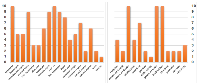
Figure 3: Semantic component number on WN18 (left) and FB13 (right).

Table 4: Different clusters in WN11 and FB13 relations.

Relation	Cluster	Triples (Head, Tail)
$\mathrm{PartOf}$	Location	(Capital of Utah, Beehive State), (Hindustan, Bharat) …
	Composition	(Monitor, Television), (Bush, Adult Body), (Cell Organ, Cell)…
$\mathrm{Religion}$	Catholicism	(Cimabue, Catholicism), (St.Catald, Catholicism) …
	Others	(Michal Czajkowsk, Islam), (Honinbo Sansa, Buddhism) …
$\mathrm{DomainRegion}$	Abstract	(Computer Science, Security System), (Computer Science, PL)..
	Specific	(Computer Science, Router), (Computer Science, Disk File) …
$\mathrm{Profession}$	Scientist	(Michael Woodruf, Surgeon), (El Lissitzky, Architect)…
	Businessman	(Enoch Pratt, Entrepreneur), (Charles Tennant, Magnate)…
	Writer	(Vlad. Gardin, Screen Writer), (John Huston, Screen Writer) …

Evaluation Protocol. We adopt the same protocol used in previous studies. For each testing triple $(h,r,t)$, we corrupt it by replacing the tail $t$ (or the head $h$) with every entity $e$ in the knowledge graph and calculate a probabilistic score of this corrupted triple $(h,r,e)$ (or $(e,r,t)$) with the score function $f_{r}(h,e)$. After ranking these scores in descending order, we obtain the rank of the original triple. There are two metrics for evaluation: the averaged rank (Mean Rank) and the proportion of testing triple whose rank is not larger than 10 (HITS@10). This is called “Raw” setting. When we filter out the corrupted triples that exist in the training, validation, or test datasets, this is the“Filter” setting. If a corrupted triple exists in the knowledge graph, ranking it ahead the original triple is also acceptable. To eliminate this case, the “Filter” setting is preferred. In both settings, a lower Mean Rank and a higher HITS@10 mean better performance.

Implementation. As the datasets are the same, we directly report the experimental results of several baselines from the literature, as in [Bordes et al., 2013], [Wang et al., 2014] and [Lin et al., 2015b]. We have attempted several settings on the validation dataset to get the best configuration. For example, we have tried the dimensions of 100, 200, 300, 400. Under the “bern.” sampling strategy, the optimal configurations are: learning rate $\alpha=0.001$, the embedding dimension $k=100$, $\gamma=2.5$, $\beta=0.05$ on WN18; $\alpha=0.0015$, $k=400$, $\gamma=3.0$, $\beta=0.1$ on FB15K. Note that all the symbols are introduced in “Methods”. We train the model until it converges in previous version (about 10,000 rounds), but we provide the results of 2,000 rounds for comparison in current version.

Results. Evaluation results on WN18 and FB15K are reported in Tab.2 and Tab.3. We observe that:

1. TransG outperforms all the baselines obviously. Compared to TransR, TransG makes improvements by 2.9% on WN18 and 26.0% on FB15K, and the averaged semantic component number on WN18 is 5.67 and that on FB15K is 8.77. This result demonstrates capturing multiple relation semantics would benefit embedding.

2. The model has a bad Mean Rank score on the WN18 and FB15K dataset. Further analysis shows that there are 24 testing triples (0.5% of the testing set) whose ranks are more than 30,000, and these few cases would lead to about 150 mean rank loss. Among these triples, there are 23 triples whose tail or head entities have never been co-occurring with the corresponding relations in the training set. In one word, there is no sufficient training data for those relations and entities.

3. Compared to CTransR, TransG solves the multiple relation semantics problem much better for two reasons. Firstly, CTransR clusters the entity pairs for a specific relation and then performs embedding for each cluster, but TransG deals with embedding and multiple relation semantics simultaneously, where the two processes can be enhanced by each other. Secondly, CTransR models a triple by only one cluster, but TransG applies a mixture to refine the embedding.

Our model is almost insensitive to the dimension if that is sufficient. For the dimensions of ${100,200,300,400}$, the HITS@10 of TransG on FB15 are ${81.8\%,84.0\%,85.8\%,88.2\%}$, while those of TransE are ${47.1\%,48.5\%,51.3\%,49.2\%}$.

4.2 Triple Classification

In order to testify the discriminative capability between true and false facts, triple classification is conducted. This is a classical task in knowledge base embedding, which aims at predicting whether a given triple $(h,r,t)$ is correct or not. WN11 and FB13 are the benchmark datasets for this task. Note that evaluation of classification needs negative samples, and the datasets have already provided negative triples.

Evaluation Protocol. The decision process is very simple as follows: for a triple $(h,r,t)$, if $f_{r}(h,t)$ is below a threshold $\sigma_{r}$, then positive; otherwise negative. The thresholds $\{\sigma_{r}\}$ are determined on the validation dataset.

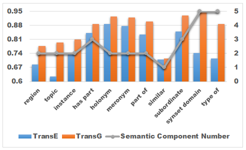
Figure 4: Accuracies of each relations in WN11 for triple classification. The right y-axis is the number of semantic components, corresponding to the lines.

Table 5: Triple classification: accuracy(%) for different embedding methods.

Methods	WN11	FB13	AVG.
LFM	73.8	84.3	79.0
NTN	70.4	87.1	78.8
TransE	75.9	81.5	78.7
TransH	78.8	83.3	81.1
TransR	85.9	82.5	84.2
CTransR	85.7	N/A	N/A
KG2E	85.4	85.3	85.4
TransG	87.4	87.3	87.4

Implementation. As all methods use the same datasets, we directly re-use the results of different methods from the literature. We have attempted several settings on the validation dataset to find the best configuration. The optimal configurations of TransG are as follows: “bern” sampling, learning rate $\alpha=0.001$, $k=50$, $\gamma=6.0$, $\beta=0.1$ on WN11, and “bern” sampling, $\alpha=0.002$, $k=400$, $\gamma=3.0$, $\beta=0.1$ on FB13.

Results. Accuracies are reported in Tab.5 and Fig.4. The following are our observations:

1. TransG outperforms all the baselines remarkably. Compared to TransR, TransG improves by 1.7% on WN11 and 5.8% on FB13, and the averaged semantic component number on WN11 is 2.63 and that on FB13 is 4.53. This result shows the benefit of capturing multiple relation semantics for a relation.

2. The relations, such as “Synset Domain” and “Type Of”, which hold more semantic components, are improved much more. In comparison, the relation “Similar” holds only one semantic component and is almost not promoted. This further demonstrates that capturing multiple relation semantics can benefit embedding.

4.3 Semantic Component Analysis

In this subsection, we analyse the number of semantic components for different relations and list the component number on the dataset WN18 and FB13 in Fig.3.

Results. As Fig. 3 and Tab. 4 show, we have the following observations:

1. Multiple semantic components are indeed necessary for most relations. Except for relations such as “Also See”, “Synset Usage” and “Gender”, all other relations have more than one semantic component.

2. Different components indeed correspond to different semantics, justifying the theoretical analysis and effectiveness of TransG. For example, “Profession” has at least three semantics: scientist-related as $\mathrm{(ElLissitzky,Architect)}$, businessman-related as $\mathrm{(EnochPratt,Entrepreneur)}$ and writer-related as $\mathrm{(Vlad.Gardin,ScreenWriter)}$.

3. WN11 and WN18 are different subsets of Wordnet. As we know, the semantic component number is decided on the triples in the dataset. Therefore, It’s reasonable that similar relations, such as “Synset Domain” and “Synset Usage” may hold different semantic numbers for WN11 and WN18.

5 Conclusion

In this paper, we propose a generative Bayesian non-parametric infinite mixture embedding model, TransG, to address a new issue, multiple relation semantics, which can be commonly seen in knowledge graph. TransG can discover the latent semantics of a relation automatically and leverage a mixture of relation components for embedding. Extensive experiments show our method achieves substantial improvements against the state-of-the-art baselines.

Support Materials. All of the related poster, slides, datasets and codes HAVE BEEN ALREADY published in http://www.ibookman.net/conference.html.

6 Code Tricks

1. The class “TransG” is the experimental version, rather than “TransG_Hierarchical”. Note that, for numerical stabilization, we fix the variance $\sigma$ as a constant.

2. When generating the new cluster, we assign the CRP factor as the mixture factor, which is required by CRP theoretically. But as to the center of new cluster, we assign a random vector rather than $\mathbf{t-h}$. Because in big data scenario, theoretical center is far away from the ground-truth.

3. Regarding the learning methodology of parameter $\pi$ and $\sigma$, we applied the stochastic gradient ascent (SGD) for efficiency, rather than likelihood counting, which is naturally suitable for CRP but inefficient. We suggest the reader to implement both for experiments.

4. Due to the slow convergence rate, in previous version, we train the model until convergence, almost around 10,000 epos. But in current version, we conduct the same rounds with other baselines （2,000 rounds).

References

- [Bollacker et al., 2008] Kurt Bollacker, Colin Evans, Praveen Paritosh, Tim Sturge, and Jamie Taylor. 2008. Freebase: a collaboratively created graph database for structuring human knowledge. In Proceedings of the 2008 ACM SIGMOD international conference on Management of data, pages 1247–1250. ACM.
- [Bordes et al., 2011] Antoine Bordes, Jason Weston, Ronan Collobert, Yoshua Bengio, et al. 2011. Learning structured embeddings of knowledge bases. In Proceedings of the Twenty-fifth AAAI Conference on Artificial Intelligence.
- [Bordes et al., 2012] Antoine Bordes, Xavier Glorot, Jason Weston, and Yoshua Bengio. 2012. Joint learning of words and meaning representations for open-text semantic parsing. In International Conference on Artificial Intelligence and Statistics, pages 127–135.
- [Bordes et al., 2013] Antoine Bordes, Nicolas Usunier, Alberto Garcia-Duran, Jason Weston, and Oksana Yakhnenko. 2013. Translating embeddings for modeling multi-relational data. In Advances in Neural Information Processing Systems, pages 2787–2795.
- [Bordes et al., 2014] Antoine Bordes, Xavier Glorot, Jason Weston, and Yoshua Bengio. 2014. A semantic matching energy function for learning with multi-relational data. Machine Learning, 94(2):233–259.
- [Collobert and Weston, 2008] Ronan Collobert and Jason Weston. 2008. A unified architecture for natural language processing: Deep neural networks with multitask learning. In Proceedings of the 25th international conference on Machine learning, pages 160–167. ACM.
- [Fan et al., 2014] Miao Fan, Qiang Zhou, Emily Chang, and Thomas Fang Zheng. 2014. Transition-based knowledge graph embedding with relational mapping properties. In Proceedings of the 28th Pacific Asia Conference on Language, Information, and Computation, pages 328–337.
- [Glorot and Bengio, 2010] Xavier Glorot and Yoshua Bengio. 2010. Understanding the difficulty of training deep feedforward neural networks. In International conference on artificial intelligence and statistics, pages 249–256.
- [Griffiths and Ghahramani, 2011] Thomas L Griffiths and Zoubin Ghahramani. 2011. The indian buffet process: An introduction and review. The Journal of Machine Learning Research, 12:1185–1224.
- [Guo et al., 2015] Shu Guo, Quan Wang, Bin Wang, Lihong Wang, and Li Guo. 2015. Semantically smooth knowledge graph embedding. In Proceedings of ACL.
- [He et al., 2015] Shizhu He, Kang Liu, Guoliang Ji, and Jun Zhao. 2015. Learning to represent knowledge graphs with gaussian embedding. In Proceedings of the 24th ACM International on Conference on Information and Knowledge Management, pages 623–632. ACM.
- [Hoffmann et al., 2011] Raphael Hoffmann, Congle Zhang, Xiao Ling, Luke Zettlemoyer, and Daniel S Weld. 2011. Knowledge-based weak supervision for information extraction of overlapping relations. In Proceedings of the 49th Annual Meeting of the Association for Computational Linguistics: Human Language Technologies-Volume 1, pages 541–550. Association for Computational Linguistics.
- [Jenatton et al., 2012] Rodolphe Jenatton, Nicolas L Roux, Antoine Bordes, and Guillaume R Obozinski. 2012. A latent factor model for highly multi-relational data. In Advances in Neural Information Processing Systems, pages 3167–3175.
- [Lin et al., 2015a] Yankai Lin, Zhiyuan Liu, and Maosong Sun. 2015a. Modeling relation paths for representation learning of knowledge bases. Proceedings of the 2015 Conference on Empirical Methods in Natural Language Processing (EMNLP). Association for Computational Linguistics.
- [Lin et al., 2015b] Yankai Lin, Zhiyuan Liu, Maosong Sun, Yang Liu, and Xuan Zhu. 2015b. Learning entity and relation embeddings for knowledge graph completion. In Proceedings of the Twenty-Ninth AAAI Conference on Artificial Intelligence.
- [Miller, 1995] George A Miller. 1995. Wordnet: a lexical database for english. Communications of the ACM, 38(11):39–41.
- [Nickel et al., 2011] Maximilian Nickel, Volker Tresp, and Hans-Peter Kriegel. 2011. A three-way model for collective learning on multi-relational data. In Proceedings of the 28th international conference on machine learning (ICML-11), pages 809–816.
- [Nickel et al., 2012] Maximilian Nickel, Volker Tresp, and Hans-Peter Kriegel. 2012. Factorizing yago: scalable machine learning for linked data. In Proceedings of the 21st international conference on World Wide Web, pages 271–280. ACM.
- [Socher et al., 2013] Richard Socher, Danqi Chen, Christopher D Manning, and Andrew Ng. 2013. Reasoning with neural tensor networks for knowledge base completion. In Advances in Neural Information Processing Systems, pages 926–934.
- [Sutskever et al., 2009] Ilya Sutskever, Joshua B Tenenbaum, and Ruslan Salakhutdinov. 2009. Modelling relational data using bayesian clustered tensor factorization. In Advances in neural information processing systems, pages 1821–1828.
- [Wang et al., 2014] Zhen Wang, Jianwen Zhang, Jianlin Feng, and Zheng Chen. 2014. Knowledge graph embedding by translating on hyperplanes. In Proceedings of the Twenty-Eighth AAAI Conference on Artificial Intelligence, pages 1112–1119.
- [Wang et al., 2015] Quan Wang, Bin Wang, and Li Guo. 2015. Knowledge base completion using embeddings and rules. In Proceedings of the 24th International Joint Conference on Artificial Intelligence.