Eta-mesic nuclei: past, present, future
Abstract
Eta-mesic nucleus or the quasibound nuclear state of an eta () meson in a nucleus is caused by strong-interaction force alone. This new type of nuclear species, which extends the landscape of nuclear physics, has been extensively studied since its prediction in 1986. In this paper, we review and analyze in great detail the models of the fundamental –nucleon interaction leading to the formation of an –mesic nucleus, the methods used in calculating the properties of a bound , and the approaches employed in the interpretation of the pertinent experimental data. In view of the successful observation of the –mesic nucleus 25Mgη and other promising experimental results, future direction in searching for more –mesic nuclei is suggested.
Keywords: Eta-mesic nuclei; Final-state interaction; Binding energy; Scattering length.
PACS Numbers:21.85+d; 21.65.Jk; 21.30.Fe; 25.40.Ve
I Introduction
It is well-known that mesons play an important role in nuclear physics. The interaction of mesons with nuclei has two complementary components: meson-induced nuclear reactions and meson-nucleus bound systems. Thus, an understanding of the ensemble of meson-nucleus interactions can enhance our knowledge of nuclear force and nuclear structure.
The modern era of meson-nucleus physics began with the advent of various meson factories in the 1960s, where high-intensity pion () and kaon () beams were made available. Since then, meson-nucleus bound systems such as –mesic and –mesic atoms have been studied extensively. Consequently, a wealth of information has been obtained about –nucleus and –nucleus interactions.
For a long time, the role of eta () meson in nuclear physics research was considered secondary because the –nucleon–nucleon () coupling constant is much smaller than the and coupling constants. In the mid-1980s, experiments at LAMPF showed that mesons are copiously produced in pion-induced nuclear reactions. This led to the development of the interaction model by Bhalerao and Liu (BL) bhal . The model has made evident that production off a nucleon is dominated by the resonance and that both the and coupling constants are by no means small. The BL model was later used by Haider and Liu to predict the existence of nuclear bound states of the meson – the –mesic nuclei hai1 .
Mesic nuclei differ from mesic atoms in two imporant aspects. While the formation of mesic atoms is driven by the Coulomb interaction between a nucleus and the bound meson, the binding of an meson into a nuclear orbit is solely due to strong interaction because the carries no electric charge. Furthermore, while the size of mesic atoms are of atomic scale, the size of –nucleus bound systems are of nuclear scale. The prediction of –mesic nucleus, a novel form of nuclear species adds, therefore, a new dimension to the study of the dynamics of –nucleus interaction and the properties of meson in nuclear medium jain ; mach .
In this paper, we review the progress made in the search of –mesic nuclei since its prediction in 1986. Among others, we examine the various experimental approaches used in the search. We also analyze in depth different methods employed in interpreting the data. In section II, we give a comprehensive analysis of the low-energy interaction models that are the basis of the formation of –mesic nucleus. In section III, theoretical calculations that led to the prediction of the existence of –mesic nuclei are reviewed. In particular, we demonstrate the importance of treating realistically the subthreshold interaction in a nucleus. Current status on experimental searches for –mesic nuclei, including the observation of –mesic nucleus 25Mgη, are discussed in section IV. Suggestions on future search for –mesic nuclei are given in section V.
II Low-energy eta-nucleon interaction
The threshold of –nucleon system is 1488 MeV which is 47 MeV below the baryon resonance . This resonance couples strongly to the system with an decay branching fraction of about 45–60%. Consequently, in the threshold region the interaction is dominated by and it is attractive. Bhalerao and Liu bhal formulated an off-shell isobar model for threshold pionic production on a nucleon and scattering. They treated the three dominant reaction channels – , , and – in a coupled-channels formalism and unitarized the model through the generation of the coupled –matrices. The parameters of the model were determined from fitting only the phase shifts and inelasticity parameters in the , and channels over a broad range of energies. With these determined parameters, the model was used to predict the cross sections and the scattering length, . The predicted scattering length has a positive real part.1 11footnotetext: The sign convention , where denotes the scattering amplitude, was used.
Because the interaction is attractive, the inequality indicates that there is no –wave –nucleon bound state newt . However, it can have an interesting nuclear implication. As will be shown in the next section, a first-order –nucleus optical potential, , is proportional to with being the –matrix of the scattering and the nuclear form factor. Consequently, leads to and, thus, to , i.e., to an attractive –nucleus interaction. The attraction, if strong enough, opens the possibility of having an bound in a nucleus to form a short-lived –nucleus bound state. Indeed, the first prediction of the existence of such nuclear bound states, the –mesic nuclei, was made by Haider and Liu hai1 .
| [fm] | Method Used111 OSE: Off-shell Extension (see the text); ChPT: Chrial Perturbation Theory; EL: Effective Lagrangian; MEM: Meson-exchange Model. | OSE | Reference |
|---|---|---|---|
| ChPT with pseudo-potential | ++ | Kaiser et al. kais1 | |
| Chiral unitary model | + | Mai et al. mai | |
| Chiral unitary approach | + | Inoue et al. inou | |
| Coupled-channel Isobars | ++ | Bhalerao and Liu bhal | |
| Coupled-channel Isobars | ++ | Bhalerao and Liu bhal | |
| Coupled-channel –matrices | ++ | Durand et al. dura | |
| Chiral EL | + | Ramon et al. ramo | |
| ChPT | + | Mai et al. mai | |
| MEM | ++ | Gasparyan et al. gasp | |
| –matrix, solution G380 | + | Arndt et al. arnd | |
| MEM | + | Sibirtsev et al. sibi | |
| Final-state interaction | – | Fäldt and Wilkin fald1 | |
| EL/–matrix | – | Feuster and Mosel feus | |
| EL/–matrix | + | Sauermann et al. saue | |
| Final-state interaction | – | Willis et al. will | |
| ChPT | + | Krippa krip | |
| Final-state interaction | – | Wilkin wilk | |
| –matrix | – | Feuster and Mosel feus | |
| ChPT with pseudo-potential | ++ | Kaiser et al. kais2 | |
| Coupled-channel T-matrices | + | Batinić al. bat1 | |
| –matrix | + | Green and Wycech gre3 | |
| ChPT | + | Nieves and Arriola niev | |
| –matrix | + | Green and Wycech gre2 | |
| –matrix | + | Green and Wycech gre4 | |
| Quark model | ++ | Arima et al. arim | |
| Vector-meson dominance | + | Lutz et al. lutz | |
| –matrix | + | Green and Wycech gre2 | |
| –matrix, solution Fit A | + | Arndt et al. arnd |
The scattering length has since been extensively studied by many researchers. In Table 1 we list some representative published results bhal ; kais1 ; mai ; inou ; dura ; ramo ; gasp ; arnd ; sibi ; fald1 ; feus ; saue ; will ; krip ; wilk ; kais2 ; bat1 ; gre3 ; niev ; gre2 ; gre4 ; arim ; lutz . Owing to the unavailibity of an beam, cannot be extracted directly from –nucleus to –nucleus elastic-scattering experiments; rather it has to be inferred from experimental data having an in the final state by way of using theoretical models.
An inspection of Table 1 shows that the values of are confined into a narrower range than that of which varies between 0.20 and 1.14 fm. The strong model dependence of is due to the fact that is not directly constrained by the data. This dependence is further evidenced by the noted large differences between the various calculated scattering lengths given in some same publications. For example, varies from 0.87 to 1.05 fm in Ref.gre2 . To emphasize the strong model dependence, Birbrair and Gridnev birb calculated using two reaction mechanisms. They showed that one of the mechanisms, the resonance mechanism, gave fm. The other mechanism, the –meson-exchange mechanism, gave fm (even the sign changed). The combined effect of the two mechanisms on the real part of the scattering length was, however, not given. We note that the –meson-exchange has also been included in some meson-exchange models (MEM) gasp ; sibi , although the individual contribution of the exchange diagram was not mentioned. In view of the result of MEM, we believe that an overall negative is unlikely.
The second column of Table 1 indicates the model or method used in determining the scattering length. The possibility of making an off-shell extension of the model/method is given in the third column of the table. An off-shell extension (OSE) of the model is particularly important for the investigation of –nucleus interaction. This is because for the formation of an –nuclear bound state, the basic interaction is off-shell. The models having both the off-shell momentum and off-shell energy dependences are indicated with a double plus sign (++) in the OSE column. Many models do not have off-shell momentum form factors. However, as the lack of an explicit off-shell momentum form factor is equivalent to an off-shell momentum form factor having an infinite range in the momentum space, these models are labeled with a single plus sign (+) so long as they can be used to calculate interaction at subthreshold energies. Otherwise, the models are labeled with a minus sign (–), as is the case with the final-state-interaction model fald1 ; wilk .
As can be seen from Table 1, many models are based on the –matrix approach arnd ; feus ; gre3 ; gre2 ; gre4 . A discussion on this approach is, therefore, in order. Within the context of the –matrix approach, one often begins by parametrizing the matrix and then relates it to the matrix by Heitler’s damping equation , where is the free Hamiltonian heit . One then uses the matrix to fit the data, whence to determine the parameters of the model. However, the data fitting can determine only the on-shell matrix and hence, by way of Heitler equation, only the on-shell matrix. In other words, models formulated within the framework of –matrix approach do not provide an explicit way of making off-momentum-shell extension. The Heitler on-shell relation has also led to the caution on the uniqueness of the off-shell matrix obtained by first extrapolating the on-shell matrix (determined from fitting data) to off-shell (subthreshold) energy region and then to infer the subthreshold matrix from the extrapolated matrix rodb .
Besides –matrix and –matrix methods, many authors applied chiral pertubation theory (ChPT) to calculate the scattering length mai ; krip ; kais2 ; niev . The results are also given in Table 1. The corresponding vary between to fm, depending on how the leading orders in the chiral expansion were calculated. However, as pointed out by Kaiser et al. kais1 , in order to investigate the formation of resonances one needs a non-perturbative approach which sums a set of diagrams to all orders. This summation is beyond the framework of systematic expansion scheme of ChPT. To overcome this difficulty, a combination of ChPT and pseudopotential methods was employed in Refs.kais1 ; kais2 . It is interesting to note that the model of Ref.kais1 is an improvement of that in Ref.kais2 and it contains more terms. This improved model leads to a smaller scattering length: fm. The authors of Ref.kais1 believe that the smaller scattering length is a result of cancellations among the various reaction diagrams in the model.
It is further noteworthy that in a recent coupled-channel isobars approach, Durand et al. dura included five meson-baryon channels and nine isobar resonances. By fitting directly the data, their model gave an fm, which is remarkably close to that given by the BL bhal model.222footnotetext: The BL model fits the phase shifts and inelasticities instead of the data.
In summary, there are compensations among contributions from various reaction mechanisms considered in the models. These mutual cancellations could be the reason that the two most recent models kais1 ; dura , which contains many reaction diagrams, give rise to a small . In this respect, we surmise that the BL model has grasped the essence of the dynamics. Clearly, the quality of the models will be ultimately determined by their predictive power of the binding energies and widths of –mesic nuclei.
III Eta-nucleus interaction and eta–mesic nucleus
The wave function of an –nucleus bound state (or an –mesic nuclear state) satisfies the eigenvalue equation , where is the Hamiltonian and is the eigenenergy. (For simplicity of notation, the quantum label will be omitted, but understood). Solving the above equation is equivalent to solving the integral equation , where is the free Green’s function. We will discuss and analyze the physics contents of three different approaches used to solve the eigenvalue equation in order to calculate the eigenenergy hai10 .
III.1 Covariant eta–nucleus optical potential
Solving a four-dimensional eigenvalue equation requires a full relativistic description of the nucleus, which is still not available at this time. Consequently, we make a covariant reduction cel1 to obtain a covariant three-dimensional equation hai1 ; hai10 :
| (3.1.1) |
Here, , , and are, respectively, the initial, final relative momentum, and the reduced mass of the –nucleus system. We denote the eigenenergy as with and representing, respectively, the binding energy and width of the –nucleus bound state. In spite of its Schrödinger-like form, Eq.(3.1.1) is fully covariant. The main advantage of working with a covariant theory is that the –nucleus interaction can be related to the elementary process by unambiguous kinematical transformations cel2 ; liu1 .
The three-dimensional covariant matrix elements in Eq.(3.1.1) is related to the fully relativistic one by
| (3.1.2) |
where
| (3.1.3) |
and
| (3.1.4) |
In Eq.(3.1.3), is the magnitude of the on-shell –nucleus relative momentum. At the –nucleus threshold, =0.
The three-dimensional relativistic wave function is related to the fully relativistic one by
| (3.1.5) |
As a result of the application of the covariant reduction, the zeroth components of the four-momenta and are no longer independent variables but are constrained by
| (3.1.6) |
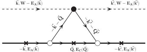
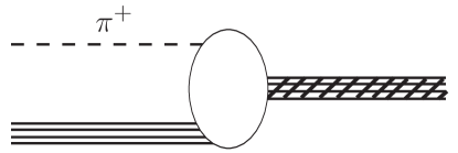
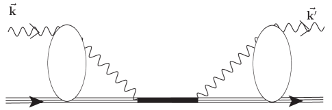
The first-order microscopic –nucleus optical potential is represented by the diagram shown in Fig.1. It can be expressed in terms of the interaction, namely,
| (3.1.7) | |||||
where the off-shell interaction is weighted by the product of the nuclear wave functions corresponding to having the nucleon at the momenta and before and after its collision with the meson, respectively. The is the invariant mass and is equal to the total energy in the c.m. frame of the and the nucleon . It is given by hai1
| (3.1.8) | |||||
where is the seperation energy of nucleon . The , , and are, respectively, the momentum, total energy, and mass of the core nucleus arising from removing a nucleon of mometum from the target nucleus of momentum . At the threshold of the –nucleus system, .
Equation (3.1.7) indicates that the calculation of involves integration over the Fermi motion variable and, hence, the matrix elements of are to be calculated at both the on-shell and off-shell momenta . On the other hand, Eq.(3.1.8) indicates that the evaluation of must be carried out at subthreshold energies.
The off-shell matrix element of in the –nucleus system is related to the off-shell scattering amplitude in the system by
| (3.1.9) | |||||
where and are the initial and final relative three-momenta in the c.m. frame of the system. As already mentioned, the kinematical transformations between the variables on the left-side and right-side of Eq.(3.1.9) are unambiguous in a three-dimensional covariant theory.
We define the on-shell limit as and , where is the on-shell relative momentum. A natural way of parameterizing is
| (3.1.10) |
so that in the on-shell limit . The has the standard partial-wave expansion of a spin 0–spin 1/2 system:
| (3.1.11) | |||||
where , , , and is the isospin of the system and equals to 1/2. In the on-shell limit,
| (3.1.12) |
The phase shifts are complex-valued because the thresholds for and reactions are lower than the threshold for scattering. When , and
| (3.1.13) |
The and are, respectively, the (complex) scattering length and volume. Near the threshold, only the –wave term, in Eq.(3.1.11), is important.
Different off-shell models give different off-shell extensions of to kinematic regions where and . In the seperable model of Ref.bhal , the off-shell amplitude is given by
| (3.1.14) |
with
| (3.1.15) |
| (3.1.16) |
and
| (3.1.17) |
Here is a short-hand notation for the quantum numbers of the isobar resonance. The is the bare mass of the isobar and , and in Eq.(3.1.17) are the self-energies of the isobar associated, respectively, with its coupling to the , , and channels bhal . The coupling constants and form factors are denoted by and . At the threshold, only the –wave interaction is important, which limits the isobar to or .
The full off-shell calculation of was carried out using the inverse-iteration method kwon and the model of Bhalerao and Liu bhal . The calculation showed that the existence of –mesic nuclei is indeed possiible hai1 . This possibility was reaffirmed by Li et al. liku who employed a different method, the Green’s function method. The results obtained with the inverse-iteration method and with improved numerical integration techniques over the Fermi motion variable of the nucleon are given in Table 2. No bound state solutions were found for nuclei with mass number . The systematic feature of having more bound states in heavier nuclei has been discussed in Ref.hai1 . In short, it is the increasing compactness of the nuclear system with the mass number as well as the increasing magnitude of that help in the formation of an –mesic nucleus. In particular, so long as the BL model bhal is used, no bound state is possible in nuclei lighter than 12C.
| Nucleus | Orbital () | |
|---|---|---|
| 12C | ||
| 16O | ||
| 26Mg | ||
| 40Ca | ||
| 90Zr | ||
| 208Pb | ||
III.2 Factorization of covariant optical potential
Once the full dynamics of the –nucleus optical potential has been understood, it is of interest to see whether more insight could be gained from using a simplified theoretical formalism. In this respect, a factorization approximation (FA) has been proposed by Liu and Haider hai10 . Within the context of FA, the scattering amplitude in Eq.(3.1.7) is taken out of the –integration at an ad-hoc fixed momentum and an ad-hoc energy :
| (3.2.1) |
where
| (3.2.2) |
is the nuclear form factor having the normalization . In Eq.(3.2.1), the off-shell is still defined by the same functional dependences on various momenta and energies as given by Eqs.(3.1.9) and (3.1.14), except that and are now replaced by and , respectively. The choice of is certainly not unique. It was suggested in Ref.hai10 to take an average of two geometries corresponding, respectively, to having a motionless target nucleon fixed before and after the collision. This leads one to set
| (3.2.3) |
This choice has, in addition, the virtue of preserving the symmetry of the –matrix with respect to the interchange of and . Because Eq.(3.1.8) shows that the interaction in a nucleus occurs at subthreshold energies, it is therefore reasonable to set
| (3.2.4) |
with being a phenomenological energy-shift parameter. From eq.(3.1.8) one sees that
| (3.2.5) |
where the average, denoted by , is over all the nucleons (j = 1,…,A). The or has the meaning of averaged binding of the target nucleons. It is worth noting that the subthreshold nature of the hadron-nucleon interaction, Eqs.(3.1.8) and (3.2.4), is also evident in –mesic and –mesic atoms. We refer to section III of Ref. hai10 for details.
In Table 3, we present the bound-state solutions obtained from using the factorized covariant potential [Eq.(3.2.1)] with MeV, and with all the other interaction parameters being the same as those for Table 2. The nuclear form factors used in the calculations are from Refs.hai10 ; hofs . A comparison between Tables 2 and 3 indicates that the FA results obtained with MeV are very close to the full dynamical calculation results. This value of is similar to the one found in pion-nucleus elastic scattering studies cott . From the results in Table 3 and from Eq.(3.2.4) we conclude that the interaction in a nucleus takes place mainly at an energy about 30 MeV below the threshold, .
| (MeV) | |||||
|---|---|---|---|---|---|
| Nucleus | Orbital () | ||||
| 12C | |||||
| 16O | |||||
| 26Mg | |||||
| 40Ca | |||||
| 90Zr | |||||
| 208Pb | |||||
III.3 Static approximation
One special case of factorized potential is the static approximation to the potential. In the static approximation, not only is the amplitude factorized out of the integration in Eq.(3.1.7), but also all the hadron masses are treated as being massive with respect to the momenta. The static approximation was first used in the study of mesic atoms eric2 , where the isospin-averaged spin-nonflip part of the first-order static optical potential for a spin-0 hadron has the general form eric
| (3.3.1) |
where is the hadron mass, the hadron-nucleus reduced mass, the effective –th partial-wave hadron-nucleon () amplitude, and is the Legendre polynomial of order . In Eq.(3.3.1), and are the initial and final hadron-nucleus relative momenta. It is instructive to see the relation between this last equation and the fully covariant amplitude, Eqs.(3.1.9)–(3.1.11). We first note that in the static approximation the target nucleon is treated as being at rest before as well as after its collision with the hadron eric2 . Hence, the initial and final relative momenta, and , in the c.m. frame of the system are and , respectively. Clearly, . In terms of the variables and , Eq.(3.3.1) becomes
| (3.3.2) |
For –mesic nuclei calculations, , , and . Hence,
| (3.3.3) |
It is easy to see that when mass of the i–th particle is treated as being very massive with respect to its momentum such that , the multiplicative factor in front of the amplitude in Eq.(3.1.9) becomes unity and that in front of the amplitude in Eq.(3.1.10) becomes
| (3.3.4) |
In mesic-atom studies, the on-shell hadron-nucleon scattering length was often used eric for in Eq.(3.3.1). We call the use of on-shell scattering length the on-shell static approximation. It was pointed out by Kwon and Tabakin kwon that should be regarded as an effective amplitude. In what follows, we will denote this effective amplitude as while use to denote exclusively the on-shell scattering length.
We show in Table 4 the calculated results given by the static approximation (SA) for light nuclei. The results of using = 0.23 + i0.09 fm (BL model bhal at 30 MeV below threshold), = 0.28 + i0.19 fm (BL model at threshold), and = 0.48 + i0.08 fm (from Fig.1 of Green-Wychech (GW) gre4 model at 30 MeV below threshold) are given, respectively, in the third, fourth, and fifth columns. We have found that the use of = 0.91 +i0.27 fm (GW model at threshold) can give bound state in 3He (result not shown). However, owing to the rapid decrease of amplitude of the GW model with the energy, one sees from Table 4 that there is no bound state in 3He when of the GW model is used.
For both the BL and GW models, . In fact, the decrease of the interaction strength at subthreshold energies is a very general feature. Furthermore, this decrease is very model dependent. Hence, it becomes impractical to employ the models listed in Table 1 for which the off-shell dependence cannot be easily reconstructed from the corresponding publications.
| (MeV) | ||||
|---|---|---|---|---|
| Nucleus | Nuclear Form Factor hofs | BL model | GW model | |
| 3He | Hollow exponential | |||
| 4He | 3-parameter Fermi | |||
| 6Li | Modified harmonic well | |||
| 9Be | Harmonic well | |||
| 10B | Harmonic well | |||
| 12C | Harmonic well | |||
| 16O | Harmonic well | |||
| 26Mg | 2-parameter Fermi | |||
Upon comparing columns 3 and 4 of Table 4 with the columns of = and = MeV of Table 3, respectively, we see that the corresponding binding energies and half-widths are quite similar to each other. This is to be expected because, as discussed above, SA is obtained from the factorization approximation in the infinite-mass limit. Quantitatively, SA gives slightly stronger binding energies. This is because in SA there is no off-shell momentum form factor at the vertices. This slight difference between the SA and FA causes a notable difference for the “boderline” nucleus. For example, while the SA predicts a loosely bound in 10B, the FA predicts no bound state in 10B. Hence, one has to exercise caution in interpreting the calculated results, particularly if the results indicate a loosely bound –mesic nucleus.
It is, thus, informative to determine the smallest value of an effective scattering amplitude, , that can bind the into the nuclear orbital in a given nucleus. Although the real and imaginary parts of this minimal off-shell amplitude are not independent of each other, we set, without loss of generality, to be 0.09 fm, as suggested by the two off-shell models (BL and GW) discussed above. We then searched for . The results are given in Table 5 for nuclei having mass number =3 to 9. We choose this mass range because of the existing strong interest in finding –nuclear bound states in light nuclear systems.
| Nucleus | Nuclear Form Factor hofs | (fm) |
|---|---|---|
| 3He | Hollow exponential | 0.49 + i0.09 |
| 4He | 3-parameter Fermi | 0.35 + i0.09 |
| 6Li | Modified harmonic well | 0.35 + i0.09 |
| 9Be | Harmonic well | 0.24 + i0.09 |
In the literature, the static approximation is sometimes referred to as the local-density approximation (LDA) in which the nucleus is treated as an infinite and motionless nuclear matter. Since the pioneering study of pionic atoms by Ericson and Ericson eric2 , the LDA has been extensively applied to studying the , and –atoms. In recent years, the method has been applied to the investigation of -mesic nucleus in 12C and heavier nuclei by Garcia-Recio et al. recio and Cieplý et al. ciep . One calculates the binding energy of the , if it exists, by solving numerically krel ; salc1 ; salc the coordinate-space Klein-Gordon equation
| (3.3.5) |
where is the self-energy of the . In Eq.(3.3.5) denotes the total energy of the and is defined by , where is the binding energy of the . The self-energy is related to the optical potential by . Theoretical models for used in Refs.recio and ciep are very different, leading to quite different results. One notes, among others, the models used in Ref.recio gave rise to very large widths while the models in Ref.ciep gave narrow . A common finding in both these references is the strong sensitivity of the calculated to the energies at which the interaction takes place. Their finding agrees with our discussion of Tables 3 to 5.
In summary, it is important to use an effective off-shell amplitude at the appropriate subthreshold energy. Since the energy dependence of the off-shell amplitude is highly model-dependent, experimental determination of the lightest nucleus in which an can be bound constitutes one of the many ways to differentiate various theoretical models.
IV Experimental search for –mesic nuclei
The unavailability of an –meson beam makes the hadron-induced nuclear production the sole way to study –nucleus interaction, including the formation of –mesic nuclei. Production of by pions peng , protons maye ; bilg ; bilg2 ; beti , and deuterons berg ; mers ; smyr have been carried out in various laboratories.
Experiments in search for –mesic nuclei can be divided into two types. In the first type of experiment one looks for a peak in the spectrum of an emerging particle as a signature of the formation of an –mesic nucleus. In the second type of experiment the bound state of is not measured and the experimental final state is composed in fact of an unbound and a nucleus. The total and differential production cross sections are measured as a function of the -nucleus relative momentum One then uses the Watson final-state-interaction method wats1 to infer from the data whether there is an –nucleus bound state.
In this section, we will discuss in detail some representative experiments in each of the above categories. Our emphasis is on the methods used for theoretical analysis of the data. For detailed technical aspects of the experiments, we refer the readers to the excellent review by Machner mach .
IV.1 Spectral methods
The first search for –mesic nucleus was carried out by Chrien et al. chri at Brookhaven National Laboratory. Targets of lithium, carbon, oxygen, and aluminum were placed in a beam at 800 MeV/c and the outgoing proton spectrum was measured. The underlying idea behind the experiment can be stated as follows liu2 . If the binding of by a nucleus takes place in the reaction
then a resonance-like peak will appear in the outgoing proton spectrum. However, the expected peak was not observed. Post-analysis has shown that the negative result was due mainly to two reasons. First, there was a huge background of proton events. Second, the was produced at high momenta, unfavorable to its capture into the nuclear orbit.
To reduce the background events, Lieb lieb has proposed to study the reaction
in an experimental setup that favors producing at rest so as to maximize its capture by the nucleus and then take advantage of the dominance ( to detect a nearly back-to-back pair in coincidence with the outgoing fast proton. A peak was observed, but it was located at the area where the detector efficiency is limited. Hence, as pointed out in Ref.mach , it is unclear whether the peak was due to the poor detector efficiency for which the data were not corrected. Nevertheless, the triple-coincidence approach proposed above has since been employed in many experimental studies and has successfully reduced background events.
(a) 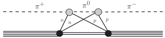
(b) 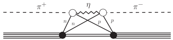
(c) 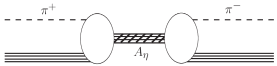
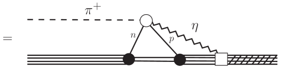
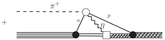
The search for an bound state in pion double-charge-exchange (DCX) reaction leading to the double isobaric analog state (DIAS), 18O()18Ne(DIAS), was carried out at LAMPF by Johnson et al. john . At pion energies above the production threshold, the DIAS can be reached via the path as well as via the path, as illustrated in Fig.2. In Fig.3 we show in detail the reaction diagrams of the –mesic nucleus formation. This LAMPF experiment was based on the theoretical calculation liu3 of the DCX reaction 14C()14O(DIAS). The calculations indicate that when there is no formation of bound state of in 14N, the interference between the amplitudes (a) and (b) shown in Fig.2 will not lead to any new structure in the excitation function of the DCX reaction. On the other hand, if there is formation of 14Nη, then the interference among the three amplitudes in Fig.2 will produce a resonance-like energy dependence in the DCX excitation function near the threshold. Furthermore, this resonance-like structure depends on the pion momentum transfer: greater is the momentum transfer, stronger will be the signature. It is reasonable to expect that the excitation functions of the DCX reactions 18ONe(DIAS) and 14CO(DIAS) have a similar energy dependence. Data analysis of the LAMPF experiment showed a visible structure in the predicted energy region of the DCX excitation function (Fig.3 of Ref.john ). However, the statistics of the data was poor. Thus, the observed structure was not statistically significant. Experiments having better statistics will be greatly valuable.
A large number of experiments designed to search for –mesic nuclei make use of transfer reactions. An example was the COSY-GEM collaboration experiment budz designed to detect the –25Mg bound state in the reaction
| (4.1.1) |
In order to maximize the probability of having the produced being captured in the nuclear orbit, the emerging 3He was detected in the forward direction (i.e., zero degree). In this forward geometry the beam momentum is entirely transfered to 3He, leaving the produced at rest. If the is bound, it cannot emerge as a free . Instead it interacts with a target nucleon and emerges as a pion. For example,
| (4.1.2) |
Because the initial has zero momentum, the emerging and would be back-to-back if the neutron had no Fermi motion. With the Fermi-motion, the and will lie in two opposite but back-to-back cones. The 3He–– triple coincidence techniques were employed to reduce background events.
The data are shown in Fig.4 where (denoted BE in Ref.budz ) represents the real part of the binding energy for events having . Events having correspond to an unbound . The experimental spectrum exhibits a peak structure centered at MeV with a half-width MeV. The significance of the peak budz is 5.3, indicating the existence of an Mg bound state, the mesic nucleus 25Mgη.

Using the factorization approach (section III.2) with MeV and the BL model bhal for , we obtained the binding energy MeV and half-width MeV for the Mg bound state hai3 . The large difference between the experimental and theoretical values of the binding energy has motivated us to reexamine how the application of a theory can take into account the actual set-up of an experiment.
The usual theoretical approach is to calculate only the following multi-step reaction process which we denote as Process M (M for mesic-nucleus formation):
25Mg
X .
However, the off-shell produced in the intermediate state can also be scattered by the residual nucleus and emerge as a pion, without being captured by the nucleus. We denote this multi-step reaction process as Process S (S for scattering):
X .
These two processes are illustrated in Fig.5. We emphasize that because these two reaction paths lead to the same measured final state, they cannot be distinguished by the experiment. Consequently, in theoretical analysis one must take coherent summation of the two amplitudes to account for the quantum interference between them. We, therefore, fit the experimental spectrum by using the sum of two amplitudes:
| (4.1.3) |
where is given by Eq.(3.2.1) and . The is the wave function of bound , and is its adjoint (p.120 of Ref.rodb ). We have noted that in the threshold and subthreshold regions, –nucleus interaction is isotropic and that the matrix elements are nearly constant for and between 0 and 100 MeV/. Because of these aspects of the –nucleus interaction and the experimental selection of events corresponding to being produced nearly at rest, Eq.(4.1.3) can be evaluated at .
(a)
(b)
’
In Eq.(4.1.3) there is only one parameter and its sole role is to adjust the overall magnitude. We emphasize that we used the same micrscopic theory-based in calculating and , and that the values of and were kept fixed, i.e., they were not fitting parameters. Furthermore, we square the sum of the amplitudes, in marked contrast to using the sum of a squared background amplitude and a squared Gaussian ampltude. Hence, interference effects between the amplitudes are present in our analysis while they were absent in the COSY-GEM fit budz .
Upon introducing the above-mentioned factorization result ( MeV and MeV) into Eq.(4.1.3), we obtained from the fit the overall scale factor (counts/fm2) and a spectral distribution peaked at MeV. The distribution is shown as curve (a) in Fig.4. The 4.0 MeV downward shift from MeV indicates clearly the importance of the interference effect. Effects of the nuclear medium modification of the interaction, in particular the true pion absorption, was also examined by Haider and Liu hai3 using the model of Chiang et al. chia . They found that the inclusion of true pion absorption gave an MeV and MeV for the process. Upon introducing these latter quantities into Eq.(4.1.3), they obtained again the same overall scale factor, (counts/fm2), and a spectral distribution peaked at –12.5 MeV (shown as curve (b) in Fig.4).
We have thus seen the importance of interference effect arising from two reaction amplitudes. It is worth emphasizing that effects of quantum interference are often crucial in understanding the data. For example, researchers were once puzzled by the observed “abnormal” cross-section ratios CNCN)] in the region. The observed ratios were later well explained when the interference between quasifree and non-quasifree reaction amplitudes was taken into account by Ohkubo and Liu ohku .
A different approach to the analysis of the COSY-GEM data on 27Al was given by Friedman et al. frie in which only the Process was considered. By using one of the strongest scattering-length models gre4 at an appropriate subthreshold energy, they were able to obtain for 25Mgη binding energies ranging from to MeV and half-widths between 1.9 and 2.9 MeV. One thus sees that the calculated peaks overestimate the observed peak ( MeV) while the calculated half-widths underestimate the observed one by a factor of two. It was argued in Ref.frie that the very small calculated width was due to the neglect of true pion-absorption contributions to in-medium amplitude. However, no quantitative estimate was given.
From the view point of nuclear theory an interesting question arises, namely, which reaction mechanism is correct? Is it the two-amplitude mechanism leading to cross sections proportional to or, is it the one-amplitude mechanism giving cross sections proportional to ? We believe that the answer lies in obtaining high-statistics data. This is because when only the process is considered, theoretical calculation will give rise to a symmetric peak centered at with a width . On the other hand, when both the and processes are included, the interference between them will result in an asymmetric peak (see both curves in Fig.4). Current data neither contradict an asymmetric peak nor rule out a symmetric one. Future high-statistics data should yield a clear answer.
Various proton- and deuteron-induced transfer-reaction experiments mach ; krze were carried out to search for bound in 3He, 4He, and 11B. To date, no bound state has been observed in these light nuclei. The photon-induced experiment
| (4.1.4) |
was performed at MAMI in Mainz pfei . A peak structure was seen near the threshold and was interpreted as an evidence of the mesic nucleus 3Heη. However, the analysis of a later experiment having much higher statistics revealed that the peak was the result of a very complicated structure of the background and, hence, could not support the previous conclusions of mesic-nucleus formation pher .
In view of our discussion on the minimum nuclear mass number needed for the formation of an –mesic nucleus (section III.2), we believe that more experiments searching for bound states of in nuclei having a mass number should be the logical next step.
IV.2 Final-state-interaction method
The differential cross section of a two-body to two-body reaction is given by
| (4.2.1) |
For nuclear production, is the –production potential, is the beam-target relative momentum in the initial channel and is the –nucleus relative momentum in the final channel, with and being the corresponding scattering wavefunctions.
Watson wats1 showed that in the threshold region, if
(a) the two-particle scattering in the final channel is dominated by –wave,
(b) the primary production (denoted ) is nearly independent of (apart from energy conservation), and
(c) the interaction between the two final particles is confined in a small region , such that ,
then the following final-state interaction (FSI) approximation holds:
| (4.2.2) |
where denotes the –wave phase shift of the two-particle scattering in the final state. In the literature, is termed the enhancement factor. The FSI approach consists in fitting the data with the following equation:
| (4.2.3) |
The low-energy expansion of is
| (4.2.4) |
with and denoting, respectively, the –nucleus –wave scattering length and effective range. In the scattering-length appproximation (SLA), one uses Hence, there are three fitting parameters, namely, and In the effective-range approximation (ERA), one uses the first two terms of Eq.(4.2.4). Consequently, there are two more fitting parameters, and . In Appendix A, we give the inequalities that and/or must satisfy when there is a quasibound state (Eqs.(A.1.19) and (A.2.14)).
Results obtained from fitting the He reaction by different groups are summarized in Table 6. (For the sake of concise notation, in this subsection the –3He scattering length and effective range will henceforth be denoted as and , respectively.) One notes from Table 6 that the results of Fits 1 and 2 cannot be used to convincingly determine whether there is an –3He bound state. This is because the sign of the real part of the scattering length are undetermined from FSI fits. Indeed, in the SLA,
| (4.2.5) |
Because in this last equation appears as a squared quantity, its sign cannot be determined. This sign ambiguity also exists in FSI fits using the ERA.
By defining and , we have
| (4.2.6) |
where , and are real-valued coefficients. From the fitted values of , and one can determine , , and , which, when combined with the given by the fit, will allow one to determine the magnitude and the sign of the product . However, one cannot determine the sign of seperately from the sign of . The authors of Ref.sibi2 believe that a clear seperation of and is only possible in a model-dependent way.
| Fits | [fm] | [fm] | [MeV/c] | Refs. |
|---|---|---|---|---|
| 1 | maye | |||
| 2 | smyr | |||
| 3 | wilk | |||
| 4 | mers | |||
| 5 | sibi2 |
In Fit 3, Wilkin wilk circumvented the sign ambiguity embedded in Eq.(4.2.5) with the aid of an optical model. First, the sign of was chosen to be positive. The sign-fixed was then used to construct a first-order –3He optical potential in the on-shell static approximation which, in turn, was used to generate . The scattering length generated in such a manner has the sign of its real part well-determined by the optical model. Finally, the and He data were fitted simultaneously by treating both the sign-fixed and as parameters. It was determined that fm and fm. By using the same procedure, it was determined from the He data that . One notes that the –3He scattering length, , does not satisfy the bound-state criteria, Eq.(A.1.19), in Appendix A-1. Hence, the result of Fit 3 indicates that there is no bound state in 3He. On the other hand, the value of given by Fit 3 suggests that an –4He bound state is possible.
For Fit 4, Mersmann et al. mers only published the value of the scattering length obtained in their effective-range approximation to FSI; the effective range in Table 6 was taken from Ref.mach . We have tested the implication of Fit 4 on the existence of –3He bound state by taking into account all possible combinations of the error bars given in the table. We found that only a small number of the combinations satisfied the existence critera of Eq.(A.2.14). However, as a whole, the result of Fit 4 could be unreliable because the high momenta part of the data used in the fit showed substantial –wave contribution mers , which is incompatible with the criteria for using Watson’s FSI theory.
The scattering length obtained in Fit 5 showed also that the sign of could not be determined by the FSI method alonesibi2 . It was pointed out in Ref.sibi2 that there were inconsistencies among the experimental data maye ; smyr ; mers ; berg . It was further suggested that one should carry out FSI fits by only using data corresponding to momentum MeV/c so as to ensure the –wave dominance (prerequisite-(a) for using the Watson FSI method).
In addition to the required wave dominance, we recall that prerequisite-(c) for using Watson’s method is that the momentum, , must satisfy . The maximal momentum, , satisfying this inequality can be determined by using the criterion wats2 . For example, the root-mean-square radius of 3He is 1.22 fm hofs . If one assumes =1.2 fm, then requires fm 70 MeV/c. The difference gives a quantitative estimate of the error of the method.
A general comment regarding the off-shell effects is in order. We see from Eq.(4.2.2) that the quantity is the on-shell –wave –nucleus scattering amplitude. In other words, the FSI method excludes off-shell information. The loss of off-shell information occured when a series of approximations wats1 ; wats2 were applied to the original scattering wave function . The on-shell feature of has also been pointed out in Refs.jain ; sibi2 . We believe that the three prerequisites leading to Eq.(4.2.2) have minimized the loss of off-shell information. In this respect, one could regard the lack of the off-shell effect as a “systematic uncertainty” intrinsic to the FSI method.
V Summary and future direction
The existence of –mesic nucleus is a consequence of the attractive interaction between meson and nucleon in the threshold energy region of the channel. This attactive force arises from the strong coupling of the baryon resonance to the system. While the strength of the attraction is not enough to cause an to be bound on a single nucleon, it can cause the to be bound on a nucleus, forming a mesic nucleus with a finite half-life. The minimum nuclear mass number for forming an –mesic nucleus depends on the predicted amplitude. The lightest nucleus onto which an can be bound clearly depends sensitively on the real part of the amplitude which is strongly model-dependent. Finding the lightest –mesic nucleus can, therefore, help differentiate various theoretical models of interaction.
We have shown in Section III that at the formation of an -mesic nucleus the meson interacts with the target nucleon at an energy that is below the threshold. Consequently, only those models that can be extended to subthreshold energies are relevant to nuclear studies of the meson.
In experimental search for –mesic nucleus, transfer reactions have been frequently employed. One such reaction has led to the observation of the –mesic nucleus with a 5.3 statistical significance budz . However, searching quasibound –nucleus states in lighter nuclei such as 3He, 4He, and 11B has not yet yielded positive results. Searching -mesic nuclei in medium-mass nuclear systems other than 25Mg is highly valuable.
A resonance structure was seen in the excitation function of the pion DCX reaction 18ONe(DIAS) at energies corresponding to threshold. However, the structure is statistically insignificant. It is, therefore, valuable to repeat this experiment with a much higher statistics. If successful, measurement of DCX excitation functions in the same energy region for other nuclei, such as 42Ca and 14C, also merit considerations.
Besides the spectral method, the FSI method has also been used to search for –mesic nucleus. However, the FSI method cannot determine the signs of the –nucleus scattering length and effective range without using a theoretical model. Hence, the conclusion of the FSI analysis is model dependent. In addition, one must bear in mind that Watson’s FSI theory wats1 is an approximative theory. The approximative feature is well laid out by the three prerequisites of the theory, as outlined in section IV-A. In particular, the dominance of final-state –wave scattering must be ascertained. In other words, the data used in FSI analyses must be isotropic in their angular distributions. This isotropy was not fulfilled in Fit 4 of Table 6. We have closely examined all the data used in the fits listed in Table 6 and found that the angular distributions are isotropic only on average (with a large disperson of 5%). Improved data are clearly helpful in future studies. To date, the FSI method has been mainly applied to3He. But no convincing evidence of bound state has been found. It is equally possible that cannot be bound onto a nucleus as light as 3He, as indicated by many models. We, therefore, believe that experiments searching for medium and heavy –mesic nuclei should be given priority in the next step of research.
Independent of whether an can be bound onto a light nucleus, studying production off a light nuclear system is important. Firstly, because in the production of a physical , the basic interaction takes place at energies above the threshold, analysis of production can, therefore, test an model in an energy domain very different from that relevant to the –mesic nucleus formation. In addition, the presence of only a few target nucleons in a light nuclear system makes calculations of multistep processes involving each individual nucleon feasible. Detailed multistep calculations have been reported for pion-induced liu4 and proton-induced lage2 ; sant productions. The production data in Ref.liu4 are well described by the Bhalerao-Liu model of interaction. Measurements of various differential cross sections of production and more microscopic analyses of the data are called for.
The existence of nuclear bound states of the in large nuclei creates the opportunity for using these mesic nuclei as a laboratory for studying the behavior of an meson in a dense nuclear environment. This is because the inner region of a medium- or heavy-mass nucleus are more close to a dense nuclear medium than the few-nucleon systems are. We mention, for example, the suggestion that bound states in nuclei are sensitive to the singlet component in and can be used as a probe of flavor-singlet dynamics bass . Hence, –mesic nuclei can improve our understanding on the – mixing. There is also theoretical work indicating that a dense nuclear medium can have very different effects on the hyperon and the baryon waas . These predicted effects can be checked by means of –mesic nuclei. There are also suggestions that the formation spectra of the –mesic nuclei can be used to check the prediction by chiral doublet theory on the mass difference betweem the nucleon and the in a nuclear medium hire ; naga .
We would like to conclude this review by emphasizing the importance of searching –nucleus bound states in medium and heavy mass nuclei. We believe that the successful observation of 25Mg, the encouraging structure in the excitation function of pion DCX reaction, the progress made in FSI studies, and the mastering of triple-coincidence and detection techniques have laid down a solid foundation for future successful searches of –mesic nuclei.
Acknowledgment
We would like to thank Dr. Christopher Aubin of Fordham University for his assistance with the reaction diagrams.
Appendix A Analytical Relations between bound-state and scattering observables
The –wave scattering amplitude is given by
| (A1) |
where is the matrix, is the phase shift, and is the c.m. momentum. For potentials that are exponentially bound, one has the following low-energy expansion:
| (A2) |
where denotes the –wave scattering length and the –wave effective range. When an optical potential is used in the calculation, the quantities , , and are all complex-valued. If there is a bound state (also termed quasibound state) of complex momentum , then the –matrix has a pole at . It follows that in Eq.(A1)
| (A3) |
In this appendix, we derive the interaction-model independent analytical relations between the binding energy, width, , scattering length , and the effective range .
A.1 The scattering length approximation
Equation (A2) shows that the first term dominates when is very small. Hence, one may approximate the low-energy expansion by using
| (A.1.1) |
Equation (A3) then gives and
| (A.1.2) |
In the complex –plane, we may express the scattering length by
| (A.1.3) |
with
| (A.1.4) |
Hence,
| (A.1.5) |
The complex energy is, therefore, given by
| (A.1.6) |
where is the reduced mass of the bound particle and
| (A.1.7) |
In the Cartesian representation,
| (A.1.8) |
where () and () denote, respectively, the binding energy and half-width of the bound state. It follows from Eqs.(A.1.3), (A.1.6), and (A.1.8) that
| (A.1.9) |
| (A.1.10) |
Because and , in what follows we will often write and whenever it is more convenient.
Because and , Eqs.(A.1.13) and (A.1.14) are, respectively, equivalent to
| (A.1.15) |
The first inequality requires In addition, a decaying outgoing wave of a bound state requires . The second inequality then leads to In summary, a bound-state requires simultaneously
| (A.1.16) |
which indicate that the bound-state poles are situated in the second quadrant (but above the diagonal line) of the complex –plane.
| (A.1.18) |
In choosing the branch of the square roots, the properties associated with the physical domains discussed above have been used. The and clearly satisfy all the three conditions stated in Eq.(A.1.16).
Equations (A.1.13) and (A.1.14) further indicate that and require, respectively, that and This in turn requires . The complex scattering length, , is therefore situated in the second quadrant but below the diagonal line in the complex -plane. In other words, in the plane the scattering length satisfies simultaneously
| (A.1.19) |
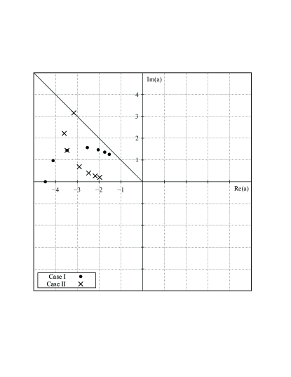
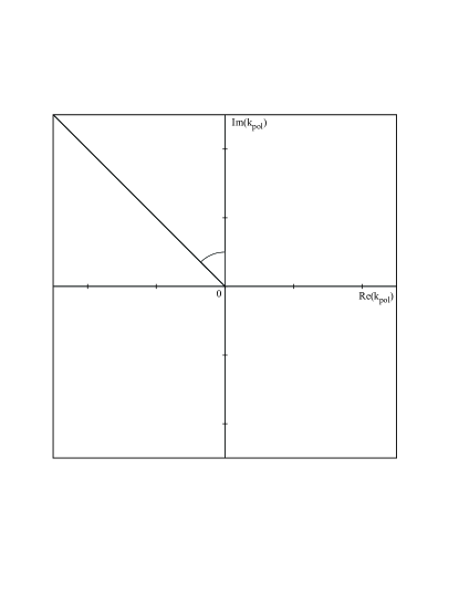
The third inequality was first given in Ref.hai10 . The physical domains in the –, –, and –planes are shown in Figs.6–8, respectively. When the polar angle, , in the –plane turns counter clockwise, the corresponding polar angles in the – and –planes turns in the opposite direction.
We now proceed to express the scattering length in terms of the binding energy . By using of Eq.(A.1.7), we can rewrite Eqs.(A.1.9) and (A.1.10) as
| (A.1.20) |
| (A.1.21) |
where, because of Eq.(A.1.8), . The inverse mapping, , is obtained by solving the above coupled equations and the result is:
| (A.1.22) |
| (A.1.23) |
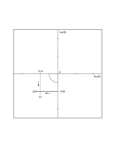
In the inverse mapping the object trajectory is on the –plane and the image trajectory is on the –plane. We have considered the following two cases as examples. Case I corresponds to fixing but varying in the direction given by the downward arrow along the dashed line in Fig.8. Case II corresponds to fixing the value of while varying along the horizontal linked-dotted line in the direction shown by the leftward arrow in Fig.8. The resulting (calculated with ) are shown, respectively, as the left-to-right solid circles and the descending crosses in Fig.6. One notes that the polar angles, , of the successive left-to-right solid circles in Fig.6 turn clockwise while the polar angles of the original –points along the downward dashed line in Fig.8 turn in a counterclockwise direction. This reversal of the sense of the turnung is a consequence of the opposite signs in front of the polar angles in Eqs.(A.1.3) and (A.1.6). The above inverse mappling explains the general feature given by detailed calculations in Ref.nisk .
Discussion on the role of nuclear mass in binding a particle: From Eqs.(A.1.22) and (A.1.23), one notes that the magnitudes of the real and imaginary parts of the scattering length are inversely proportional to . For –mesic nucleus, is the reduced mass of , which increases as nuclear mass increases. This in turn indicates that for to have a given binding energy in a lighter nucleus, it requires a larger than that for to have the same binding energy in heavier nuclei.
Finally, it is worth pointing out that in the literature, another sign convention of the scattering length is also used, namely, lim. We showed in Ref.hai4 that this sign difference does not alter the obtained results.
A.2 The effective range approximation
In the effective-range approximation to the low-energy expansion, both the first and second terms of Eq.(A2) are retained and Eq.(A3) becomes
| (A.2.1) |
There are three variables, and in this equation. Conseqently, one can only express one of the three variables as a function of the other two. By writing
| (A.2.2) |
one obtains readily from Eq.(A.2.1)
| (A.2.3) |
| (A.2.4) |
where
| (A.2.5) |
It is easy to verify that when , Eq.(A.2.5) becomes , and Eqs.(A.2.3) and (A.2.4) reduce to Eqs.(A.1.22) and (A.1.23), respectively.
By treating as the unknown in Eq.(A.2.1), we have the relations
| (A.2.6) |
| (A.2.7) |
Finally, we solve for when and are known. As one can see, Eq.(A.2.1) yields two solutions for . However, only the following one is physically meaningful, namely,
| (A.2.8) |
This is because as , so that the scattering-length approximation is recovered. It follows from Eq.(A.2.8) that
| (A.2.9) |
If , we can make a Taylor’s expansion of the square root. To the order of , Eqs.(A.2.8) and (A.2.9) are, respectively, equal to
| (A.2.10) |
| (A.2.11) |
The condition is then given by
| (A.2.12) |
or
| (A.2.13) |
This last inequality, resulting from the use of limited Taylor expansion, was first given in Ref.sibi2 . Consequently, in the effective-range approximation the necessary conditions for having a bound state are:
| (A.2.14) |
where and are obtained from taking, respectively, the imaginary and real parts of Eq.(A.2.10). When is very large, either the Taylor’s expansion cannot be done or it brings no advantage. In this latter case, we can directly calculate Eq.(A.2.8) by using the polar representation.
| (A.2.18) |
From Eqs.(A.2.16)–(A.2.18), one readily obtains
| (A.2.19) |
Again, for a bound state to exist, the quantities and must satisfy the three inequalities of Eq.(A.1.16).
In summary, all the analytic expressions derived in this appendix are interaction-model independent as long as the potential of the particle-target interaction belongs to the class of exponentially bound potentials so that the low-energy expansion, Eq.(A2), can be made. The only kinematic approximation used in our derivation is which is a very good approximation for bound state problems. We emphasize that the model depedence of the interaction dynamics does come into play when one theoretically calculates the scattering length, , the effective range, , and the binding energies, . In the effective-range approximation when two of these three quantities are calculated (or measured), the remaining one will be fixed by the analytic relations. Similarly, in the scattering-length approximation, when (or ) is calculated (or measured), the other variable (or ) will be fixed by the analytic relation. In this respect, these analytic relations can be used to check the consistency of calculations (or measurements).
References
References
- (1) R.S. Bhalerao and L.C. Liu, Phys. Rev. Lett. 54, 865 (1985).
- (2) Q. Haider and L.C. Liu, Phys. Lett. B 172, 257 (1986); B 174, 465E (1986).
- (3) N.G. Kelkar, K.P. Khemchandani, N.J. Upadhyay, and B.K. Jain, Rep. Prog. Phys. 76, 066301 (2013).
- (4) H. Machner, J. Phys. G 42, 043001 (2015).
- (5) Roger G. Newton, Scattering Theory of Waves andParticles ( Springer-Verlag, N. Y., 1982). The scattering length defined in this reference has an opposite sign to the one used in this work. This sign difference has been taken into account in our discussion.
- (6) N. Kaiser, T. Waas, and W. Weise, Nucl. Phys. A 612, 297 (1997).
- (7) M. Mai, P.C. Bruns, and U-G Meiner, Phys. Rev. D 86, 094033 (2012).
- (8) T. Inoue, E. Oset, and M.J. Vicente Vacas, Phys. Rev. C 65, 035204 (2002).
- (9) J. Durand, B. Juliá-Díaz, T.-S. H. Lee, B. Saghai, and T. Sato, Phys. Rev.C 78, 025204 (2008)
- (10) J. Caro Ramon, N. Kaiser, S. Wetzel, and W. Weise, Nucl. Phys. A 672, 249 (2000).
- (11) A.M. Gasparyan, J. Haidenbauer, C. Hanhart, and J. Speth, Phys. Rev. C 68, 045207 (2003).
- (12) R.A. Arndt et al., Phys. Rev. C 72, 045202 (2005).
- (13) A. Sibirtsev et al., Phys. Rev. C 65 044007 (2002).
- (14) G. Fäldt and C. Wilkin, Nucl. Phys. A 587, 769 (1995).
- (15) T. Feuster and U. Mosel, Phys. Rev. C 58, 457 (1998).
- (16) Ch. Sauermann, B.L. Friman, and W. Nörenberg, Phys. Lett. B 341, 261 (1995).
- (17) N. Willis et al., Phys. Lett. B 406, 14 (1997).
- (18) B. Krippa, Phys. Rev. C 64, 047602 (2001)
- (19) C.W. Wilkin, Phys. Rev. C 47, R938 (1993).
- (20) N. Kaiser, P.B. Siegel, and W. Weise, Phys. Lett. B 362, 23 (1995).
- (21) M. Batinić, I. Dadić, I. Šlaus, A. Švarc, B.M.K. Nefkens, and T.-S. H. Lee, Phys. Scripta 58, 15 (1998).
- (22) A.M. Green and S. Wycech, Phys. Rev. C 55, R2167 (1997).
- (23) J. Nieves and E.R. Arriola, Phys. Rev. D 64, 116008 (2001).
- (24) A.M. Green and S. Wycech, Phys. Rev. C 60, 035208 (1999).
- (25) A.M. Green and S. Wycech, Phys. Rev. C 71, 014001 (2006).
- (26) M. Arima, K. Shimizu, and K. Yazaki, Nucl. Phys. A 543, 613 (1992).
- (27) M.F.M. Lutz, G. Wolf, and B. Friman, Nucl. Phys. A 706, 431 (2002); erratum: Nucl. Phys. A 765, 495 (2006).
- (28) B.L. Birbrair and A.B. Gridnev, Z. Phys. A 354 95 (1996).
- (29) W. Heitler, Proc. Cambridge Phil. Soc. 37, 291 (1941); Elementary Wave Mechanics, Oxford University Press, Oxford, 1961.
- (30) L.S. Rodberg and R.M. Thaler, Introduction in Quantum Theory of Scattering, Academic Press, New York (1967), pp.238-239.
- (31) Q. Haider and L.C. Liu, Phys. Rev. C 66, 045208 (2002).
- (32) L.S. Celenza, M.K. Liou, L.C. Liu, and C.M. Shakin, Phys. Rev. C 10, 398 (1974). Used the -reduction with . Note that there is a misprint in the first line of Eq.(12), where should have been .
- (33) L. Celenza, L.C. Liu, and C.M. Shakin, Phys. Rev. C 12, 1983 (1975).
- (34) L.C. Liu and C.M. Shakin, Prog. Part. and Nucl. Phys. 5, 207 (1980).
- (35) Y.R. Kwon and F.B. Tabakin, Phys. Rev. C 18, 932 (1978).
- (36) G.L. Li, W.K. Cheng, and T.T.S. Kuo, Phys. Lett. B 195, 515 (1987).
- (37) H.R. Collard, L.R.B. Elton, and R. Hofstader, Numerical Data and Functional Relationships in Science and Technology, Vol. 2, ed. H. Schopper (Springer-Verlag, N.Y., 1967).
- (38) W.B. Cottingame and D.B. Holtkamp, Phys. Rev. Lett. 45, 1828 (1980).
- (39) M. Ericson and T.E.O. Ericson, Ann. Phys. 36, 323 (1966).
- (40) T.E.O. Ericson and F. Scheck, Nucl. Phys. B 19, 450 (1970); See Eq.(18) given therein.
- (41) C. García-Recio, T. Inoue, J. Nieves, and E. Oset, Phys. Lett. B 550, 47 (2002).
- (42) A. Cieplý, E. Friedman, A. Gal, and J. Mares̆, Nucl. Phys. A 925, 126 (2014).
- (43) M. Krell and T.E.O. Ericson, J. Compu. Phys. 3 202 (1968).
- (44) E. Oset and L.L. Salcedo, Anales de Fisica, Serie A 80, 109 (1984).
- (45) E. Oset and L.L. Salcedo, J. Compu. Phys. 57, 361 (1985).
- (46) J.C. Peng et al., Phys. Rev. Lett. 63, 2353 (1989).
- (47) B. Mayer et al., Phys. Rev. Phys. Rev. C 53, 2068 (1996).
- (48) R. Bilger et al., Phys. Rev. C 65, 044608 (2002).
- (49) R. Bilger et al., Phys. Rev. C 69, 014003 (2004).
- (50) M. Betigeri et al., Phys. Lett. B 472, 267 (2000).
- (51) J. Berger et al., Phys. Rev. Lett. 61, 919 (1988).
- (52) J. Smyrski et al., Phys. Lett. B 649, 258 (2007).
- (53) T. Mersmann et al., Phys. Rev. Lett. 98, 242301 (2007).
- (54) K.M. Watson, Phys. Rev. 88, 1164 (1952).
- (55) R.E. Chrien et al., Phys. Rev. Lett. 60, 2595 (1988).
- (56) L.C. Liu and Q. Haider, Phys. Rev. C 34, 1845 (1986).
- (57) B.J. Lieb et al., Progress at LAMPF, Los Alamos National Laboratory Report No. LA-11670-PR, 1989, p.52.
- (58) J.D. Johnson et al., Phys. Rev. C47, 2571 (1993).
- (59) Q. Haider and L.C. Liu, Phys. Rev. C36, 1636 (1987).
- (60) A. Budzanowski et al., Phys. Rev. C 79, 012201(R) (2009).
- (61) Q. Haider and L.C. Liu, J. Phys. G 37, 125104 (2010).
- (62) H.C. Chiang, E. Oset, and L.C. Liu, Phys. Rev. C 44, 738 (1991).
- (63) Y. Ohkubo and L.C. Liu, Phys. Rev. C 30, 254 (1984).
- (64) E. Friedman, A. Gal, and J. Mares̆, Phys. Lett. B 725, 334 (2013).
- (65) W. Krzemien, P. Moskal, and M. Skurzok, Acta Phys. Pol. B 46, 757 (2015).
- (66) M. Pfeiffer et al., Phys. Rev. Lett. 92, 252001 (2004); Phys. Rev. Lett. 94, 049102 (2005).
- (67) F. Pheron et al., Phys. Lett. B 709, 21 (2005).
- (68) A. Sibirtsev, J. Haidenbauer, C. Hanhart, and J. A. Niskanen, Eur. Phys. J. A 22, 495 (2004).
- (69) M.L. Goldberger and K.M. Watson, Collision Theory, John Wiley & Sons, Inc., New York, 1964, Chapter 9.
- (70) L.C. Liu, Phys. Lett. B 288, 18 (1992).
- (71) J.M. Laget and J.F. Lecolley, Phys. Rev. Lett 61, 2069 (1988).
- (72) A.B. Santra and B.K. Jain, Phys. Rev. C 64, 025201 (2001).
- (73) S.D. Bass and A.W. Thomas, Phys. Lett. B 634, 368 (2006); Acta Phys. Pol. B 45, 627 (2014).
- (74) T. Waas and W. Weise, Nucl. Phys. A 625, 287 (1997).
- (75) S. Hirenzaki and H. Nagahiro, Acta Phys. Pol. B 45, 619 (2014).
- (76) H. Nagahiro, D. Jido, and S. Hirenzaki, Phys. Rev. C 80, 025205 (2009), and the references therein.
- (77) J.A. Niskanen and H. Machner, Nucl. Phys. A 902, 40 (2013).
- (78) Q. Haider and Lon-chang Liu, Acta Phys. Pol. B 45, 827 (2014).