Kinematic dipole detection with galaxy surveys: forecasts and requirements

Abstract

Upcoming or future deep galaxy samples with wide sky coverage can provide independent measurement of the kinematic dipole – our motion relative to the rest frame defined by the large-scale structure. Such a measurement would present an important test of the standard cosmological model, as the standard model predicts the galaxy measurement should precisely agree with the existing precise measurements made using the CMB. However, the required statistical precision to measure the kinematic dipole typically makes the measurement susceptible to bias from the presence of the local-structure-induced dipole contamination. In order to minimize the latter, a sufficiently deep survey is required. We forecast both the statistical error and the systematic bias in the kinematic dipole measurements. We find that a survey covering $\sim 75\%$ of the sky in both hemispheres and having $\sim 30$ million galaxies can detect the kinematic dipole at $5\sigma$, while its median redshift should be at least $z_{\rm med}\sim 0.75$ for negligible bias from the local structure.

1. Introduction

Measurements of the motion of our Solar System through the cosmic microwave background (CMB) rest frame represent one of the early successes of precision cosmology. This so-called kinematic dipole corresponds to a velocity of $(369\pm 0.9)\,{\rm km\,s^{-1}}$ in the direction $(l,b)=(263.99^{\circ}\pm 0.14^{\circ},48.26^{\circ}\pm 0.03^{\circ})$ (Hinshaw et al., 2009). The kinematic dipole has even been detected (though not as precisely measured) by observing the relativistic aberration in the CMB anisotropy that it causes, which is detected via the coupling of high CMB multipoles in Planck (Aghanim et al., 2014).

Independently, the past few decades have seen significant progress in measuring the dipole in the distribution of extragalactic sources. The contribution of our motion through the large-scale structure (LSS) rest frame – the kinematic dipole – also leads to relativistic aberration, this time of galaxies or other observed LSS sources. We define the dipole amplitude via the amount of its “bunching up” of galaxies in the direction of the dipole

$$\frac{\delta N({\bf\hat{n}})}{\bar{N}}=A\,\bf\hat{d}\cdot\bf\hat{n}+\epsilon(\hat{n}),$$ (1)

where $N$ is the galaxy number in an arbitrary direction ${\bf\hat{n}}$, ${\bf\hat{d}}$ is the dipole direction, and $\epsilon$ is random noise. The dipole amplitude $A$ is approximately (but not exactly) equal to our velocity through the LSS rest frame in units of the speed of light; the precise relation is given in the following section.

However, the dominant contribution to the LSS dipole is typically not our motion through the LSS rest frame, but rather the fluctuations in structure due to the finite depth of the survey. The dipole component of the latter – the so-called “local-structure dipole” in the nomenclature of Gibelyou & Huterer (2012) – has amplitude $A\sim 0.1$ for shallow surveys extending to $z_{\rm max}\sim 0.1$, but is significantly smaller for deeper surveys. The local-structure dipole is the dominant signal at multipole $\ell=1$ in all extant LSS surveys. It has been measured and reported either explicitly (Baleisis et al., 1998; Blake & Wall, 2002; Hirata, 2009; Gibelyou & Huterer, 2012; Fernández-Cobos et al., 2014; Rubart & Schwarz, 2013; Yoon et al., 2014; Appleby & Shafieloo, 2014; Alonso et al., 2015), or as part of the angular power spectrum measurements. No LSS survey completed to date therefore had a chance to separate the small kinematic signal from the larger local-structure dipole contamination due to insufficient depth and sky coverage. This will change drastically with the new generation of wide, deep surveys.

Standard theory based on the adiabatic initial perturbations predicts that the kinematic dipole measured by the LSS should agree with the one measured by the CMB. Detection of an anomalously large (or small) dipole or the disagreement of its direction from that of the CMB dipole could indicate new physics: for example, the presence of superhorizon fluctuations in the presence of isocurvature fluctuations (Turner, 1991; Zibin & Scott, 2008; Itoh et al., 2010; Erickcek et al., 2008). Clearly, a kinematic dipole detection and measurement represent an important and fundamental consistency test of the standard cosmological model.

2. Methodology

2.1. Theoretical signal

The expected LSS kinematic dipole signal amplitude is given by (Burles & Rappaport, 2006; Itoh et al., 2010)

$$A=2\tilde{\beta}=2[1+1.25x(1-p)]\beta$$ (2)

where $\beta=v/c=0.00123$ (assuming the CMB dipole). The contribution $2\beta$ comes from relativistic aberration, while the correction $[1+1.25x(1-p)]$ corresponds to the Doppler effect; here $x$ is the faint-end slope of the source counts, $x\equiv d\log_{10}[n(m<m_{\rm lim})]/dm_{\rm lim}$, and $p$ is the logarithmic slope of the intrinsic flux density power-law, $S_{\rm rest}(\nu)\propto\nu^{p}$.

Clearly, the parameters $x$ and $p$ depend on the population of sources selected by the survey, and on any population drifts as a function of magnitude. We now estimate these parameters – note also that we only need the quantity $A$ to set our fiducial model, so very precise values of the population parameters are not crucial for this paper. Marchesini et al. (2012) find that the faint end of the V-band galaxy luminosity function does not vary much over the redshift range $0.4\leq z\leq 4$ and is equal to, in our notation, $x=0.11\pm 0.02$. Moreover, for optical sources the flux density slope $p$ varies significantly with the age of the source, but in the infrared it is more consistent, with measurements indicating $p\sim 0$ (White & Majumdar, 2004; Mo et al., 2010). Here we adopt $p=0$. Applying all these values to Eq. (2), we get

$$A\simeq 0.0028\quad\mbox{(expectation from CMB)}.$$ (3)

While the actual value of the kinematic dipole is of course unknown prior to the measurement, standard cosmology theory predicts it takes this value, plus or minus O(20%) changes depending on the source population selected. We adopt Eq. (3) as the fiducial amplitude.

The fiducial direction we adopt is the one of the best-fit CMB dipole, $(l,b)=(263.99^{\circ},48.26^{\circ})$. Note, however, that the results may vary depending on the relative orientation between the actual dipole direction and the coverage of the observed sky. Finally, note that bias (of the galaxy clustering relative to the dark matter field) enters into the contamination of the kinematic dipole measurements, but not the signal. The former quantity – the local-structure dipole – is linearly proportional to the bias $b$. Therefore, the bigger the bias, the more contamination the local-structure dipole provides for measurements of the kinematic effect. In this work we assume bias of $b=1$. Note that the kinematic signal itself, being due to our velocity through the LSS rest frame, is independent of bias.

2.2. Statistical error

Rewriting Eq. (1) somewhat, the modulation in the number of sources is given at each direction ${\bf\hat{n}}$ can be written as

$$\frac{\delta N(\hat{n})}{\bar{N}}={\bf x}\cdot{\bf T(\hat{n})}+\epsilon(\hat{n}),$$ (4)

where ${\bf x}=(d_{x},d_{y},d_{z},k_{1},...,k_{M})$ is the vector of the three dipole component coefficients in the three spatial coordinates, plus coefficients corresponding to other multipoles (one for the monopole, five for that many components of the quadrupole, etc), as well as any desired systematic templates. The vector ${\bf T(\hat{n})}=(n_{x},n_{y},n_{z},t_{1}(\hat{n}),...,t_{M}(\hat{n}))$, contains the three dipole unit vectors (with $n_{x}^{2}+n_{y}^{2}+n_{z}^{2}=1$), plus $M$ additional spatial patters for all templates included. Note that the choice of the fiducial values of the non-dipole template coefficients $k_{i}$ is arbitrary, since we will fully marginalize over each of these, effectively allowing $k_{i}$ to vary from zero to plus infinity. The optimal estimate of x is given by ${\bf\hat{x}}=F^{-1}g$ (Hirata, 2009), where the components of the vector $g$ are $g_{i}=\int T_{i}(\hat{n})\delta N^{\Omega}(\hat{n})d^{2}\hat{n}$ and the best-fit dipole ${\bf d_{best}}$ is given by the first three elements of ${\bf x}$. Here the Fisher matrix $F$ is given by

$$F_{ij}=\bar{N}^{\Omega}\int T_{i}(\hat{n})T_{j}(\hat{n})d^{2}\hat{n},$$ (5)

where $N^{\Omega}\equiv dN/d\Omega$ is the number of galaxies per steradian and $\Omega$ is a solid angle. Note that the Fisher information is proportional to the number of sources, and unrelated to the depth of the survey. It is therefore the number of sources, together with the sky cut (not just the fraction of the sky observed $f_{\rm sky}$ but also the shape of the observed region relative to the multipoles that need to be extracted) that fully determines the statistical error in the various templates including the dipole.

The Fisher matrix contains information about how well the three Cartesian dipole components, as well as the multipole moments of all other components, can be measured in a given survey. Our parameter space has a total of $M_{\rm par}=(\ell_{\rm max}+1)^{2}$ parameters, where $\ell_{\rm max}$ is the maximum multipole included to generate the templates (see below for more on the choice of $\ell_{\rm max}$). With this Fisher matrix in hand, we then marginalize over the $M\equiv M_{\rm par}-3$ non-dipole parameters, using standard Fisher techniques, to get the $3\times 3$ Fisher matrix describing the final inverse covariance matrix for the dipole components. Finally, we perform a basis change, converting from Cartesian coordinates $\{d_{x},d_{y},d_{z}\}$ to spherical coordinates $\{A,\theta,\phi\}$ (where $A$ is the amplitude of dipole), by using a Jacobian transformation to obtain the desired $3\times 3$ Fisher matrix in the latter space, $F^{\rm marg}_{(3\times 3)}$. The forecasted error on $A$ is then given in terms of this matrix as

$$\sigma(A)=\sqrt{[(F^{\rm marg}_{(3\times 3)})^{-1}]_{AA}}.$$ (6)

In a realistic survey with partial-sky coverage, the presence of other multipoles (monopole, quadrupole, etc) will be degenerate with the dipole, degrading the accuracy in determining the latter. We have extensively tested for this degradation, in particular with respect to how many multipoles need to be kept – that is, what value of $\ell_{\rm max}$ (and therefore $M$) to adopt. We explicitly found that the prior information on the “nuisance” $C_{\ell}$, corresponding to how well they can be (and are being) independently measured, is of key value: once the prior information on the $C_{\ell}$ – corresponding to cosmic variance plus measurement error – is added, very high multipoles are not degenerate with the dipole. Our tests show that keeping all multipoles out to $\ell_{\rm max}=10$ is sufficient for the dipole error to fully converge. We also experimented with adding additional individual templates $t_{i}({\bf\hat{n}})$ corresponding to actual sky systematics and with modified coverage (corresponding to e.g. dust mask around the Galactic plane), but found that these lead to negligible changes in the results. Moreover, we envisage a situation where the maps have already been largely cleaned of stars by the judicious choice of color cuts prior to the dipole search analysis. For these two reasons, we choose not to include any additional systematic templates in the analysis.

2.3. Systematic bias

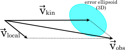
Figure 1.— Sketch of the problem at hand: we would like to measure the kinematic dipole $\vec{v}_{\rm kin}$, whose error (represented by a cyan ellipse) can be calculated given the number of extragalactic objects and the sky coverage. The LSS local dipole, $\vec{v}_{\rm local}$, provides a bias in this measurement. For a survey deep enough (and depending somewhat on the direction of its $\vec{v}_{\rm local}$), bias in the measurement of $\vec{v}_{\rm kin}$ will be smaller than the statistical error.

The local-structure dipole ${\bf d}_{\rm local}$ will also provide a contribution to the kinematic signal ${\bf d}_{\rm kin}$ that we seek to measure. The observed dipole in any survey will be the sum of the two contributions:

$${\bf d}_{\rm obs}={\bf d}_{\rm kin}+{\bf d}_{\rm local}.$$ (7)

Without any loss of generality, we consider the kinematic dipole as the fiducial signal in the map, whose errors are therefore given by the Fisher matrix worked out above. We consider the local-structure dipole to represent the contaminant whose magnitude, ideally, should be such that the resulting observed dipole ${\bf d}_{\rm obs}$ is still within the error ellipsoid around the kinematic dipole direction and amplitude. This is illustrated in Fig. 1.

We now quantify the systematic bias, due to the local structure, relative to statistical error in the measurements of the kinematic dipole. First note that we are in possession of the (statistical) inverse covariance matrix for measurements of the kinematic dipole, $F^{\rm marg}_{(3\times 3)}$, which is already fully marginalized over other templates. The quantity

$$\Delta\chi^{2}({\bf d}_{\rm local}) = ({\bf d}_{\rm obs}-{\bf d}_{\rm kin})^{T}F^{\rm marg}_{(3\times 3)}({\bf d}_{\rm obs}-{\bf d}_{\rm kin})$$ (8)

$$= {\bf d}_{\rm local}^{T}F^{\rm marg}_{(3\times 3)}{\bf d}_{\rm local}$$

then represents “(bias/error)²” in the kinematic dipole measurement due to the presence of the local-structure contamination. This chi squared depends quadratically on the expected local-structure dipole, and is therefore expected to sharply drop with deeper surveys which have a lower $|{\bf d}_{\rm local}|$, as we find in the next section. With three parameters, requiring 68% confidence level departure implies $\Delta\chi^{2}=3.5$. We therefore require that, for a given survey, the local-structure dipole magnitude and direction are such that the value in Eq. (8) is smaller than this value.

3. Results

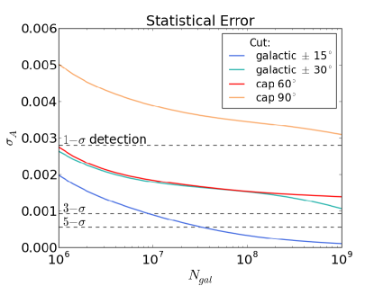
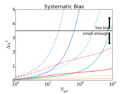
Figure 2.— Left panel: Statistical error in the dipole amplitude, marginalized over direction and other multipoles that are coupled to the dipole, as a function of the number of galaxies in a survey. The top horizontal dashed line shows the amplitude expected based on the CMB dipole measurements ($A=0.0028$), and is the fiducial value in this work. The two dashed horizontal lines show the $3\sigma$ and $5\sigma$ detection of dipole with the fiducial amplitude. Right panel: $\Delta\chi^{2}$, defined in Eq. (8), corresponding to the bias from the local-structure dipole, as a function of the number of objects $N_{\rm gal}$. For a fixed amplitude of ${\bf d}_{\rm local}$ the $\Delta\chi^{2}$ still depends on the direction of this vector; here we show the value averaged over all directions of ${\bf d}_{\rm local}$. Solid lines show cases when the median galaxy redshift is $z_{\rm med}=1.0$, while dashed lines are for $z_{\rm med}=0.75$. The legend colors are the same in the left panel.

For a fixed sky cut and number of sources in the survey, we first calculate the error on the amplitude of the dipole $\sigma(A)$. In the left panel of Fig. 2 we show errors as a function of the number of galaxies in a survey. As previously noted, this statistical error does not depend on the depth of the survey, but does depend on both $f_{\rm sky}$ and the shape of the sky coverage. Here we show results for an isolatitude cut around the equator of $\pm 15\deg$, and $\pm 30\deg$ and isolatitude cap-shaped cuts of $90\deg$ (i.e. half the sky removed) and $60\deg$ (i.e. leaving out a circular region around a pole). Note that the Galactic $\pm 15\deg$ cut and the cap cut of $60\deg$ both have $f_{\rm sky}=0.75$, while the Galactic $\pm 30\deg$ and the cap $90\deg$ cuts both have $f_{\rm sky}=0.5$. The results will also depend on the fiducial amplitude of the dipole, and here and throughout we assume the CMB-predicted value of $A=0.0028$. Even for a fixed $f_{\rm sky}$ of the survey, the cut geometry clearly matters, and the Galactic-cut cases have a smaller error in the dipole amplitude due to symmetrical covering of the two hemispheres. For Galactic $\pm 15\deg$ case, 3-$\sigma$ and 5-$\sigma$ detections are easily achievable, requiring only $N_{\rm gal}=9\times 10^{6}$ and $3\times 10^{7}$ objects, respectively. Note that if the actual direction of the LSS kinematic dipole deviates from the assumed dipole direction (the CMB direction), the result changes. For a 5-sigma detection and the same $\pm 15\deg$ isolatitude cut, a dipole pointing along toward a Galactic pole, which is the best-case scenario, only requires 8 million objects; if instead the dipole points toward the Galactic plane, then 70 million objects are required. For the Galactic $\pm 30\deg$ cut, the 3-$\sigma$ detection is more challenging since it requires having over $N_{\rm gal}=10^{9}$ sources. The cap $60\deg$ cut mostly follows the trend of the Galactic $\pm 30$ case. Lastly, the $90\deg$ cap cut cannot detect the signal even at the 1-sigma level and with $N_{\rm gal}=10^{9}$. We conclude that dual-hemisphere sky coverage is crucial in the ability of the survey – or a combined collection of surveys – to detect the kinematic dipole.

The right panel of Fig. 2 shows the systematic bias in the dipole measurement due to the presence of the local-structure contamination, showing the quantity defined in Eq. (8). Because ${\bf d}_{\rm local}$ has an a-priori unknown direction and its amplitude changes according to the depth of the survey, the systematic error is a function of direction of ${\bf d}_{\rm local}$ and the depth of the survey. Therefore, we choose to plot $\Delta\chi^{2}$ averaged over all directions of ${\bf d}_{\rm local}$.

To calculate the amplitude of ${\bf d}_{\rm local}$, we model the radial distribution of objects as $n(z)=z^{2}/(2z_{0}^{3})\exp(-z/z_{0})$ (Huterer, 2002), where the parameter $z_{0}$ is related to the median redshift as $z_{0}=z_{\rm med}/2.674$. A deeper survey (larger $z_{0}$) has a smaller local-structure dipole. Note that one could additionally cut out low-redshift objects in order to further reduce the contamination from the nearby structures, as well as the star-galaxy confusion; we have not done that here.

The dashed lines in the right panel of Fig. 2 represent the cases when $z_{\rm med}=0.75$ and the solid ones are when $z_{\rm med}=1.0$. Since $\Delta\chi^{2}$ is inversely proportional to the statistical error squared, the best cases in the left panel of Fig. 2 have a larger bias in the right panel. In particular, the more galaxies the survey has, the more it is susceptible to systematic bias (for a fixed depth and thus $|{\bf d}_{\rm local}|$). For example, a survey with $\pm 15\deg$ Galactic cut with 30 million sources can detect the kinematic dipole at 5-$\sigma$, but needs to have a median redshift of at least $z_{\rm med}=0.75$ in order for this not to be excessively biased due to local structures.

On the whole, Fig. 2 indicates that the convincing detection of the kinematic dipole expected given the CMB measurements is entirely within reach of future surveys, as long as those surveys have good coverage over both hemispheres and, given the source density, are deep enough not to be biased by the local-structure dipole. All requirements can be straightforwardly satisfied by surveys like some combination of LSST (Ivezic et al., 2008), Euclid (Laureijs et al., 2011) and DESI (Levi et al., 2013) and, especially, by deep, all-sky surveys with good redshift information such as SPHEREX (Doré et al., 2014).

Finally, we have also calculated the statistical error in the direction of the kinematic dipole, based on the fiducial amplitude we had adopted. The direction’s error is generally rather large, e.g. an area of about $\simeq 10\deg$ in radius for $N_{\rm gal}=10^{8}$ and the Galactic $\pm 15\deg$ cut. Nevertheless, a combination of the kinematic dipole’s amplitude and direction that roughly match the CMB dipole would present a convincing confirmation of the standard assumption. One could further carry out detailed forecasts of what various findings could rule out the null hypothesis; we leave that for future work.

4. Conclusions

We have studied the prospects for measuring the kinematic dipole – our motion through the LSS rest frame – as revealed by the relativistic aberration of tracers of the large-scale structure. The standard theory predicts that the kinematic dipole should agree with the CMB dipole, but this expectation could be violated due to a number of reasons. Therefore, verifying the standard expectation is an important null test in cosmology. The challenge comes from the fact that the dipole amplitude is small ($A\sim 0.003$), and easily contaminated by the intrinsic clustering of galaxies (the “local-structure dipole”).

A successful measurement of the kinematic dipole therefore has two qualitatively different requirements: the survey should cover most of the sky and have enough objects to have sufficient signal-to-noise to detect the aberration signature of the dipole, but it should also be deep enough, so that the local-structure dipole contamination is sufficiently small. The two requirements are displayed in the two panels of Fig. 2 respectively. For a 5-$\sigma$ detection, a survey covering $\gtrsim 75\%$ of the sky in both hemispheres (our “Galactic $\pm 15\deg$ cut” case), with $N_{\rm gal}\gtrsim 30$ million galaxies, is required. For a negligible bias, this same survey should have median redshift greater than about $0.75$ or higher, with increasing depth requirements as $N_{\rm gal}$ increases.

Fortunately these requirements can be satisfied by upcoming surveys, including DESI, Euclid, and LSST if they are combined, and potentially with SPHEREX alone. Even current all-sky surveys such as WISE (Wide-field Infrared Survey Explorer, Wright et al. (2010)) are not out of the question, provided a sufficiently deep sample can be selected photometrically; current WISE samples have typical galaxy redshifts $z_{\rm med}\simeq 0.2$ (Bilicki et al., 2014) and are not yet deep enough to measure the kinematic dipole.

References

- Aghanim et al. (2014) Aghanim, N., et al. 2014, A&A, 571, A27
- Alonso et al. (2015) Alonso, D., Salvador, A. I., Sánchez, F. J., & et al. 2015, MNRAS, 449, 670
- Appleby & Shafieloo (2014) Appleby, S., & Shafieloo, A. 2014, JCAP, 10, 70
- Baleisis et al. (1998) Baleisis, A., Lahav, O., Loan, A. J., & Wall, J. V. 1998, MNRAS, 297, 545
- Bilicki et al. (2014) Bilicki, M., Jarrett, T. H., Peacock, J. A., Cluver, M. E., & Steward, L. 2014, ApJS, 210, 9
- Blake & Wall (2002) Blake, C., & Wall, J. 2002, Natur, 416, 150
- Burles & Rappaport (2006) Burles, S., & Rappaport, S. 2006, ApJL, 641, L1
- Doré et al. (2014) Doré, O., et al. 2014, arXiv:1412.4872
- Erickcek et al. (2008) Erickcek, A., Carroll, S., & Kamionkowski, M. 2008, PhRvD, 78, 083012
- Fernández-Cobos et al. (2014) Fernández-Cobos, R., Vielva, P., Pietrobon, D., & et al. 2014, MNRAS, 441, 2392
- Gibelyou & Huterer (2012) Gibelyou, C., & Huterer, D. 2012, MNRAS, 427, 1994
- Hinshaw et al. (2009) Hinshaw, G., et al. 2009, ApJS, 180, 225
- Hirata (2009) Hirata, C. M. 2009, JCAP, 0909, 011
- Huterer (2002) Huterer, D. 2002, PhRvD, 65, 063001
- Itoh et al. (2010) Itoh, Y., Yahata, K., & Takada, M. 2010, PhRvD, 82, 043530
- Ivezic et al. (2008) Ivezic, Z., Tyson, J. A., Allsman, R., Andrew, J., & Angel, R. 2008, arXiv:0805.2366
- Laureijs et al. (2011) Laureijs, R., et al. 2011, arXiv:1110.3193
- Levi et al. (2013) Levi, M., et al. 2013, arXiv:1308.0847
- Marchesini et al. (2012) Marchesini, D., Stefanon, M., Brammer, G. B., & Whitaker, K. E. 2012, ApJ, 748, 126
- Mo et al. (2010) Mo, H., van den Bosch, F., & White, S. 2010, Galaxy Formation and Evolution (Cambridge University Press)
- Rubart & Schwarz (2013) Rubart, M., & Schwarz, D. J. 2013, A&A, 555, A117
- Turner (1991) Turner, M. 1991, PhRvD, 44, 3737
- White & Majumdar (2004) White, M., & Majumdar, S. 2004, ApJ, 602, 565
- Wright et al. (2010) Wright, E. L., et al. 2010, AJ, 140, 1868
- Yoon et al. (2014) Yoon, M., Huterer, D., Gibelyou, C., Kovács, A., & Szapudi, I. 2014, MNRAS, 445, L60
- Zibin & Scott (2008) Zibin, J., & Scott, D. 2008, PhRvD, 78, 123529