How the quantum ring shape influences its energy spectrum

Abstract

We propose a new approach for modeling the quantum ring single particle energy spectrum. The approach is based on separation of variables in the Schrödinger equation in oblate spheroidal coordinates. We consider a model of a spheroidal quantum ring with infinite walls. Our simple model allowed us to study the spectra for quantum rings of different shapes. The spectrum is calculated for the ground and several excited states and the ring shape dependence of the spectrum is demonstrated. The spectrum can demonstrate parabolic or non-parabolic dependence on the magnetic quantum number for different shapes of the ring profile.

I Introduction

Quantum dots and quantum rings are becoming irreplaceable components of modern electronics due to the arising technological opportunity to control their spectral properties accurately. Such structures as multiple concentric nano-rings, rings around a quantum dot and many other complex nano-objects are been fabricated on the base of droplet epitaxy SelfOrgQRFabrication ; DotRingFabrication ; MultiRingsFabrication . Fabrication methods for creating regular two- and three-dimensional structures of nano-rings are also being developed on the base of nanospherical lithography RingArrays1 ; 3DNanoArrays ; ColloidalTemplate .

Despite an obvious progress in fabricating nano-objects, however, the researchers still meet a challenge of their efficient theoretical description. Even for single-particle states, we have an alternative: either to restrict ourselves to oversimplified one-dimensional models chaplik , or to resort to computationally costly calculations for taking into account the three-dimensional structure of the systems Voskoboynikov ; filikhin . In this work we suggest an approach which on the one hand allows us to treat quite complex three-dimensional ring-shaped nano-structures, and on the other hand to reduce the computational cost of the model by exact separation of variables in oblate spheroidal coordinates.

The major goal of this work is to demonstrate suitability of oblate spheroidal coordinates for describing three-dimensional nano-scale quantum rings using a simple model of a particle confined to a ring-like structure by an infinite potential wall. This approach not only allowed us to develop a computationally simple scheme for ring spectrum calculations, but also to study the dependence of such spectra on the shape of the ring.

It is worth mentioning that J. Even and S. Loualiche Even have also considered a model of a quantum ring bounded by an infinite potential wall. In their case, the boundary of the ring is formed by circular paraboloids and the separation of variables is performed in parabolic coordinates. The advantage of our approach over their is that it allows us to vary the shape of the ring while fixing the volume and the characteristic size $R$ of the ring, which, basically, has made our study possible. In our approach it is also possible to model a flat substrate directly without solving an auxiliary problem for a symmetric ring and post-selecting the solutions that fit the required boundary condition.

It is well known, that the two types of the spheroidal coordinates – prolate and oblate – both admit separation of variables for the Schrödinger equation kom_pon_sla ; morse_fesh . Even though there are only a few known quantum problems with exact separation of variables, it is the prolate spheroidal coordinates that are preferably used in hundreds of published researches. The oblate spheroidal coordinates, however, have been used rather rarely in quantum mechanical calculations. There are only a few such papers known to the authors. The most famous example is, probably, the the work of Rainwater Rainwater , where the model of a spheroidal infinitely deep potential well made it possible to explain magnetic moments of many nuclei based on the behavior of an unpaired nucleon. In this letter we demonstrate how the use of oblate spheroidal coordinates allowed us to make some curious observations on the variations of quantum ring spectra as the ring shape changes.

We employ a very simplified model of a single particle in a quantum ring. Assuming a very sharp transition between inner and outer regions of the quantum well we can neglect the effective mass inhomogeneity. As we are interested in qualitative properties of the particle confined in a ring, we use natural units (n.u.) of energy such that the Schrödinger equation for a free particle takes the following form

$$\frac{1}{2}\Delta\Psi+E\Psi=0\,.$$ (1)

We introduce oblate spheroidal coordinates$(\xi,\eta,\varphi)$

$$\begin{array}[]{l}x=\frac{R}{2}\sqrt{(\xi^{2}+1)(1-\eta^{2})}\cos{\varphi},\\ y=\frac{R}{2}\sqrt{(\xi^{2}+1)(1-\eta^{2})}\sin{\varphi},\\ z=\frac{R}{2}\xi\eta,\\ \xi\in[0,\infty),\;\;\;\eta\in[-1,1],\;\;\;\varphi\in[0,2\pi).\end{array}$$ (2)

We shall require the quantum well to be bounded by the coordinate surfaces $\xi=\xi_{0}$, $\eta=\eta_{0}$ and the plane $\xi=0$, $\eta=0$ which corresponds to a flat substrate. In Fig. 1 we show a cross section of the coordinate surfaces, and the corresponding three-dimensional configuration of the ring is shown in Fig. 2. Other – even more complex – combinations of coordinate surfaces can also be employed.

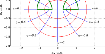
Figure 1: Oblate spheroidal coordinate surfaces projection to $(x,z)$-plane with $z$ as the symmetry axis. The bold contour corresponds to a cross section of the quantum ring boundary. The three-dimensional shape of the ring is given by rotating around the $z$ axis by the angle $0\leq\theta\leq 2\pi$. (Color online).

Figure 2: Isometric projection of a quantum ring, a rectangular segment is taken off to demonstrate the cross section.

By putting zero boundary conditions at the surface of the ring Fig. 2 we confine the particle inside the ring. Given this boundary conditions the wave function $\Psi_{j}$ corresponding to the energy $E_{j}$ can be represented as a product

$$\Psi_{j}(\xi,\eta,\varphi;R)=N_{kqm}(R)X_{mk}(\xi;R)Y_{mq}(\eta;R)e^{im\varphi}\,,$$ (3)

where the multi-index $j=\{kqm\}$ stands for a set of quantum numbers $k$, $q$ and $m$ such that $k$ and $q$ give the number of roots of the corresponding functions in $\xi$ and $\eta$, while the magnetic quantum number $m$ takes the values of $0,\pm 1,\pm 2,\dots$. The normalization constant $N_{kqm}(R)$ can be determined from the condition

$$\int_{V}\Psi_{kqm}^{\ast}(\xi,\eta,\varphi;R)\Psi_{k^{\prime}q^{\prime}m^{\prime}}(\xi,\eta,\varphi;R)dV=\delta_{kk^{\prime}}\delta_{qq^{\prime}}\delta_{mm^{\prime}}\,,$$ (4)

where $dV=\frac{R^{3}}{8}(\xi^{2}+\eta^{2})d\xi d\eta d\varphi$ is the volume element in oblate spheroidal coordinates.

Substituting (3) into (1) we obtain a system of ordinary differential equations kom_pon_sla

$$\begin{array}[]{rcl}\frac{d}{d\xi}(\xi^{2}+1)\frac{d}{d\xi}X_{mk}(\xi;R)&-\\ -\left[\lambda-p^{2}(\xi^{2}+1)-\frac{m^{2}}{\xi^{2}+1}\right]X_{mk}(\xi;R)&=&0\,,\end{array}$$ (5)

$$\begin{array}[]{rcl}\frac{d}{d\eta}(1-\eta^{2})\frac{d}{d\eta}Y_{mq}(\eta;R)&+\\ +\left[\widetilde{\lambda}-p^{2}(1-\eta^{2})-\frac{m^{2}}{1-\eta^{2}}\right]Y_{mq}(\eta;R)&=&0\,.\end{array}$$ (6)

subject to boundary conditions $X_{mk}(0;R)=X_{mk}(\xi_{0};R)=0$ and $Y_{mq}(0;R)=Y_{mq}(\eta_{0};R)=0.$ Here $p_{j}^{2}=\frac{E_{j}R^{2}}{2}\,$ is the energy parameter, $\lambda=\lambda_{mk}^{(\xi)}(p)$ and $\widetilde{\lambda}=\lambda_{mq}^{(\eta)}(p)$ are the separation constants. The energy spectrum is determined from the separation constant matching condition

$$\lambda_{mk}^{(\xi)}(p)=\lambda_{mq}^{(\eta)}(p)\,.$$ (7)

Obviously, the spectrum scales as an inversed square of the characteristic ring size $R.$

Consider a set of rings of a fixed volume $V$

$$V=\frac{\pi R^{3}}{4}\int\limits_{0}^{\xi_{0}}\int\limits_{0}^{\eta_{0}}(\xi^{2}+\eta^{2})d\xi d\eta=\frac{\pi R^{3}}{12}\xi_{0}\eta_{0}(\xi_{0}^{2}+\eta_{0}^{2})\,.$$ (8)

Evidently, the parameters of the ring $\xi_{0}$ and $\eta_{0}$ enter this formula symmetrically. The ranges for $\xi$ and $\eta$, however, and the corresponding coordinate surfaces are different (Fig. 1). We can, thus, fix the volume and the characteristic radius of the ring in (8) and obtain a relationship between $\xi_{0}$ and $\eta_{0}$ $\xi_{0}=f(\eta_{0})$ which keeps the volume of the structure invariant. This way our approach allows us to study the influence of the ring shape on the structure of its spectrum.

The shape of the ring, however, is not managed by the parameter $\eta_{0}$ alone. Even though the spectrum of the model scales as the inversed square of the characteristic size of the ring $1/R^{2}$, this scaling breaks if we keep the volume of the ring fixed. So in order to make a comprehensive study of the ring shape effects, we should also vary the volume of the ring or its characteristic size. As the ring volume scales exactly as $R^{3}$, it is just natural to introduce a dimensionless parameter $\sigma=\frac{V^{1/3}}{R}$ and use it as the second independent shape parameter.

We illustrate the variations of the ring shape for different values of shape parameters $\eta_{0}$ and $\sigma$ in Fig. 3. We can identify several distinctive cases. For smaller values of $\eta_{0}$ and bigger values of $\sigma$ the ring surface is dominated by the hyperboloid inside the ring with nearly cylindrical section of the ellipsoid outside the ring. As $\eta_{0}$ approaches 1 for smaller $\sigma$ we see the picture reversed: the major part of the boundary is formed by the ellipsoid outside with a nearly cylindrical section of the hyperboloid inside the ring. For bigger $\sigma$ the ring looks like an ellipsoid with a hole. When the both shape parameters are small the ring looks like a one-dimensional structure.

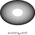
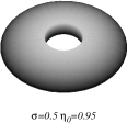
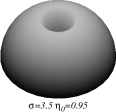
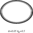
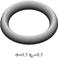
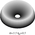
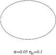
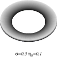
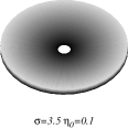
Figure 3: Ring shapes for different shape parameters $\eta_{0}$ and $\sigma$.

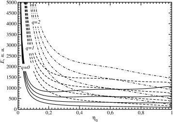
Figure 4: Energy dependence $E_{kq0}=E_{kq0}(\eta_{0})$ on the shape parameter $\eta_{0}$ for the ground and the lowest 11 excited states for $\sigma=0.5$, $R=1$.

In Fig. 4 we show the energy dependence $E_{j}(\eta_{0})$ on the shape parameter $\eta_{0}$ for 12 lowest eigenstates of the ring. As $\eta_{0}\rightarrow 0$ the ring is getting flat, and the energy spectrum starts becoming degenerate in quantum number $k$ as the corresponding degree of freedom contributes less and less to the total energy. It is also noteworthy that some of the curves $E_{j}(\eta_{0})$ have minima. This newly discovered observation might have some implications for ring fabrication techniques.

Another, and, probably, more interesting example of the quantum ring spectrum shape dependence is the study of excitations in magnetic quantum number $m$. It is usually assumed that the spectrum of angular excitations in a quantum ring can be described by a simple one-dimensional model which predicts parabolic behavior of the excited states $E_{m}\propto m^{2}$ Viefers . Our calculations, however, clearly demonstrate essential deviations from this rather common assumption.

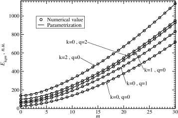
Figure 5: Quantum ring excitations and their fits for $V=1/2$, $R=1$ and $\eta_{0}=0.95$.

$kq$	$\eta_{0}=0.1$	$\eta_{0}=0.5$	$\eta_{0}=0.95$
00	$200.9+0.16\ m^{1.99}$	$47.9+0.66\ m^{1.88}$	$26.1+2.46\ m^{1.66}$
01	$700.8+0.14\ m^{2.00}$	$127.8+0.50\ m^{1.96}$	$56.7+3.33\ m^{1.60}$
02	$1491.0+0.14\ m^{2.00}$	$242.8+0.46\ m^{1.97}$	$98.9+3.85\ m^{1.59}$
10	$262.4+0.19\ m^{1.99}$	$100.2+0.79\ m^{1.88}$	$70.8+3.99\ m^{1.58}$
20	$323.6+0.21\ m^{1.97}$	$170.9+0.79\ m^{1.91}$	$137.0+5.31\ m^{1.54}$

Table 1: Parametrization $\epsilon_{kqm}=\epsilon_{kq0}+\alpha_{kq}m^{\beta_{kq}}$ of the spectra for the rings of different shapes for $V=1/2$ and $R=1$.

Consider rings of different shapes as shown at Fig. 3 at a fixed volume and calculate the lowest excitations $E_{kqm}$ for $(kq)=(00),(01),(02),(10),(20)$ and $|m|=0,1,\ldots,30.$ These energy levels are smooth functions of the quantum number $m,$ and their dependence on $m$ is easy to fit with a simple parametrization $\epsilon_{kqm}=\epsilon_{kq0}+\alpha_{kq}m^{\beta_{kq}}$ as is shown in Fig. 5. The one-dimensional ring model corresponds to $\beta_{kq}\equiv 2,$ and the deviations of $\beta$ from this value indicate that the quantum ring is essentially three-dimensional and should not be treated as a bended quantum wire. As an example, we present the parametrization of the quantum ring spectra for three different shape configurations in Table 1. In the case of a flat ring ($\eta_{0}=0.1,$) we see that all the calculated states demonstrate the parabolic $m$ dependence, and this ring configuration essentially follows the one-dimensional model. For the other two configurations, however, the value of $\beta$ is measurably smaller than 2, and the one-dimensional model of the ring does not describe the energy spectrum of the "magnetic" excitations. In Fig. 6 we show a contour map for the magnetic spectrum shape parameter $\beta_{00}$ as a function of the ring shape parameters $\eta_{0}$ and $\sigma.$ The maps for higher $k$ and $q$ have similar structure. The map demonstrates several interesting features.

First, there is a clear tendency for flat ring configurations ($\eta_{0}<0.125$) to produce $m$-dependence of the spectrum very close to the textbook $m^{2}$ behavior of 1D models. The configurations with more prominent 3D structure ($\eta_{0}>0.4$) generally produce spectra that deviate from the 1D model quite substantially.

Second, the configurations of small $\sigma$ follow 1D-like dependence on the magnetic quantum number $m$ for a broader range of configurations independent, basically, of the parameter $\eta_{0}.$ This is not surprising, as these configurations do look like as a 1D wire loop for smaller $\eta_{0}$ and become flat as $\eta_{0}$ increases.

Finally, there is a special set of shapes about $\sigma\approx 0.45$ and $\eta_{0}>0.95$ for which the deviation of the spectrum $m$-dependence from the 1D model is the most prominent. It is interesting to note that in the vicinity of this region we also see rapid change in the behavior of the spectrum from purely parabolic to non-parabolic while the variations of the ring shapes are rather small.

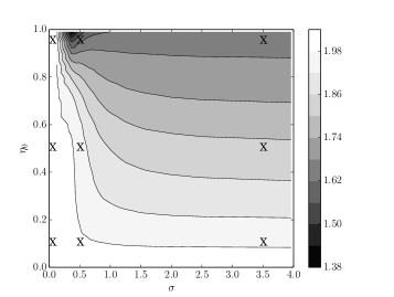
Figure 6: The magnetic quantum number excitation spectrum shape characteristic $\beta_{00}$ for rings of different shapes. The marked points correspond to the ring configurations in Fig. 3.

The use of oblate spheroidal coordinates for quantum ring calculations allowed us to discover a nontrivial shape dependence of the ring spectrum properties.

In this article we studied the model of a quantum ring formed in a potential well with infinite walls. We have shown that the corresponding Schrödinger equation admits separation of variables in oblate spheroidal coordinates. This allowed us to construct a classification of single-particle states in the quantum ring and to demonstrate essential dependence of the single-particle spectrum on the shape of the quantum ring. In particular, the most demonstrating example of such shape dependence can be seen by studying the dependence of the spectrum on the magnetic quantum number. We see, that a rather common assumption of parabolic dependence of 1D model should not be taken for granted, and quantum rings of many shapes that resemble realistic configurations are expected to demonstrate the spectra that scale as $m^{\beta}$ with $1.3<\beta<2.$

Obviously, the model need further refinements to be employed in quantitative studies. The first step towards more elaborated models would rely on the existence of potentials that admit separation of variables in oblate spheroidal coordinates while reproducing the interaction of a particle with the nano-structure of interest. Fortunately, there are known classes of potentials that fit this description, and we are planning to study such potential models in the nearest future. Studying the interactions of spheroidal quantum rings with external fields that do not break the symmetry of the system also seems an interesting direction of research.

References

- (1) A. Lorke, J. M. Garcia, R. Blossey, R. J. Luyken, P. M. Petroff, Adv. Solid State Phys., 43, 125 (2003).
- (2) C. Somaschini, S. Bietti, N. Koguchi, S. Sanguinetti, Nanotechnology, 22, 185602 (2011).
- (3) C. Somaschini, S. Bietti, S. Sanguinetti, N. Koguchi, A. Fedorov, M. Abbarchi, M. Gurioli, IOP Conf. Series: Materials Science and Engineering, 6, 012008 (2009).
- (4) J. Wu, Z. M. Wang, K. Holmes, E. Marega Jr., Z. Zhou, H. Li, Yu. I. Mazur, G. J. Salamo, Appl. Phys. Lett., 100, 203117 (2012).
- (5) H. Yabu, Langmuir, 29, (4), 1005 (2013).
- (6) Y. Li, G. T. Duan, G. Y. Liu, W. P. Cai, Chem. Soc. Rev., 42, 3614 (2013).
- (7) L. I. Magarill, D. A. Romanov, A. V. Chaplik, Zh. Eks. Teor. Fiz., 110, 669 (1996).
- (8) Y. Li, O. Voskoboynikov, C. P. Lee, Tech. Proc. of the 2002 Inter. Conf. on Modeling and Simulation of Microsystems / Nanotech, 1, 540 (2002).
- (9) I. Filikhin, E. Deyneka, H. Melikyan, B. Vlahovic, Molecular Simulation, 31, 779 (2005).
- (10) J. Even, S. Loualiche, J. Phys. A, 37, 289 (2004).
- (11) I. V. Komarov, L. I. Ponomarev, and S. Yu. Slavyanov, Spheroidal and Coulomb Spheroidal Functions, (Nauka, Moscow, 1976) [in Russian].
- (12) P. M. Morse, and H. Feshbach, Methods of Theoretical Physics, (McGraw-Hill, New York, 1953).
- (13) J. Rainwater, Phys. Rev., 79, 432 (1950).
- (14) S. Viefers, P. Koskinen, Deo P. Singha, and M. Manninen, Physica E, 21, 1 (2004).