SLICING BLACK HOLE SPACETIMES

Abstract

A general framework is developed to investigate the properties of useful choices of stationary spacelike slicings of stationary spacetimes whose congruences of timelike orthogonal trajectories are interpreted as the world lines of an associated family of observers, the kinematical properties of which in turn may be used to geometrically characterize the original slicings. On the other hand properties of the slicings themselves can directly characterize their utility motivated instead by other considerations like the initial value and evolution problems in the 3-plus-1 approach to general relativity. An attempt is made to categorize the various slicing conditions or “time gauges” used in the literature for the most familiar stationary spacetimes: black holes and their flat spacetime limit.

1 Introduction

A century after the birth of general relativity, we now take for granted the existence of various stationary spacelike slicings of stationary spacetimes which have certain special geometrical properties useful in studying the astrophysical consequences of say, black hole spacetimes. Many of these slicings arise from geometrical properties of their irrotational congruences of orthogonal timelike trajectories, interpreted as the world lines of an associated family of observers which may be either geodesic or accelerated. Other slicings are instead characterized by the intrinsic or extrinsic geometry of the slicing itself. We here survey the various categories of such useful slicings for nonrotating and rotating black hole spacetimes, but starting with the limiting flat Minkowski spacetime which allows the greatest variety of examples of special slicings.

Among the observer-defined slicings of black hole spacetimes is the Boyer-Lindquist time coordinate slicing associated with the usual stationary accelerated observers referred to equivalently as fiducial or locally non-rotating or zero angular momentum observers, abbreviated as FIDOs, LNOs or ZAMOs. Geodesic observer families instead characterize the rain, drip and hail coordinate systems [1, 2] which include the Painlevé-Gullstrand coordinates [3, 4] and their generalizations [5]. For nonrotating black holes the latter are also characterized by the intrinsic curvature properties of their associated slicing, whose induced geometry is flat. Smarr and York [6] pioneered linking the preservation of kinematical properties of the slicing to the choice of time lines in an evolving spacetime, while constant mean curvature slicings were seen as privileged from the point of view of the initial value problem even earlier [7, 8, 9]. Special spherically symmetric slicings of the nonrotating Schwarzschild black hole spacetime were first considered by Estabrook et al [10, 11]. Recent work has investigated the geometry associated with analogue black holes [12, 13] and shown that neither intrinsically flat nor conformally flat slicings of the Kerr spacetime exist [14, 15, 16, 5].

On the other hand, the analysis of the Cauchy problem of general relativity has also led to the introduction of spacetime slicings useful in simplifying the evolution equations, like harmonic slicing [17] (and closely related time gauges [18]), defined by requiring the time coordinate of the spacetime associated with the slicing to be a harmonic function. Furthermore, the numerical relativity study of multi-black hole dynamics [19] takes advantage of the use of “hyperbolic slicings,” requiring spatial compactification techniques at infinity [20, 21, 22], as well as horizon penetrating coordinates like Painlevé-Gullstrand coordinates. We refer to these as “analytic slicings,” belonging to the Cauchy problem literature, in contrast with those of a “geometrical” nature.

Motivated primarily by a desire to better understand the underlying geometrical structure of these spacetimes, we systematically review, develop and discuss special slicings of black hole spacetimes together with their flat Minkowski limit. We use geometric units with $c=1=G$. Greek indices run from $0$ to $3$ and refer to spacetime quantities, while Latin indices from $1$ to $3$ and refer to spatial quantities.

2 Spacetime, general coordinates and spacelike $3$-surfaces

Let $\{t,x^{a}\}$ be a generic set of coordinates adapted to a slicing of spacetime by spacelike hypersurfaces of constant values of the time coordinate $t$ and write the metric as

$${}^{(4)}{\rm d}s^{2}=g_{\alpha\beta}{\rm d}x^{\alpha}{\rm d}x^{\beta}=g_{tt}{\rm d}t^{2}+2g_{ta}{\rm d}t{{\rm d}x}^{a}+g_{ab}{\rm d}x^{a}{\rm d}x^{b},\qquad(a,b=1,2,3)\,.$$ (1)

The convenient Wheeler lapse-shift notation [23] re-expresses the metric in the form

$${}^{(4)}{\rm d}s^{2} = -N^{2}{\rm d}t^{2}+g_{ab}({\rm d}x^{a}+N^{a}{\rm d}t)({\rm d}x^{b}+N^{b}{\rm d}t)$$ (2)

$$\equiv -N^{2}{\rm d}t^{2}+g_{ab}\omega^{a}\omega^{b}\,,$$

defining the lapse function $N$ and shift vector field $N^{c}$ which satisfy

$$g_{tt}=-(N^{2}-N_{c}N^{c})\,,\qquad g_{ta}=N_{a}=g_{ab}N^{b}\,,$$ (3)

while the 1-forms $\{\omega^{a}\}$ are orthogonal to the unit timelike 1-form $n^{\flat}=-N{\rm d}t$ associated with the unit normal vector field $n$ to the slicing

$$n=\frac{1}{N}(\partial_{t}-N^{a}\partial_{a})\,.$$ (4)

Here we use the equivalent shortened notations for the the spatial coordinate frame $\partial_{a}\equiv\partial_{x^{a}}\equiv e_{a}$. The induced Riemannian $3$-metric on the time slices is simply

$${}^{(3)}\kern-1.5pt{\rm d}s^{2}=g_{ab}{\rm d}x^{a}{\rm d}x^{b}\,,$$ (5)

with spacetime volume element $\sqrt{-g}=N\sqrt{{\rm det}(g_{ab})}$. Note that $\{N\,dt,\omega^{a}\}$ is the dual frame to the frame $\{n,\partial_{a}\}$ reflecting the orthogonal decomposition of each tangent space adapted to the slicing and its normal direction.

For a stationary spacetime, one can choose these coordinates so that the stationary symmetry corresponds to translation in the time coordinate $t$, with associated Killing vector field $\partial_{t}$. To transform to another stationary slicing, without loss of generality one can consider restricted choices of the new spacelike time coordinate of the form

$$T=t-f(x^{1},x^{2},x^{3})$$ (6)

which retain the time lines of the original coordinate system if the spatial coordinates are not changed. One is still free to choose new time lines by changing the spatial coordinates as well, but unless the time lines are associated with a Killing vector field, the metric will become explicitly time-dependent.

On a generic slice $\Sigma$ of the new slicing, the 1-form

$${\rm d}T={\rm d}t-f_{a}{\rm d}x^{a}\,,\qquad f_{a}=\partial_{a}f\,,$$ (7)

vanishes identically, i.e.,

$${\rm d}T\big{|}_{\Sigma}=0\quad\rightarrow\quad{\rm d}t=f_{a}{\rm d}x^{a}\quad({\rm on}\,\,\Sigma)\,.$$ (8)

If we retain the spatial coordinates and only introduce this new time coordinate,

$$t=T+f(X^{1},X^{2},X^{3}),\qquad x^{a}=X^{a},$$ (9)

then one must distinguish the spatial coordinate frame vector fields tangent to the old and new time coordinate hypersurfaces

$$\partial_{T}=\partial_{t}\,,\qquad E_{a}\equiv\partial_{X^{a}}=\partial_{a}+f_{a}\partial_{t}\,,\qquad{\rm d}X^{a}={\rm d}x^{a}\,.$$ (10)

Re-expressing the spacetime metric then leads to

$${}^{(4)}{\rm d}s^{2} = -L^{2}{\rm d}T^{2}+h_{ab}({\rm d}X^{a}+L^{a}{\rm d}T)({\rm d}X^{b}+L^{b}{\rm d}T)\,,$$ (11)

$$\equiv -L^{2}{\rm d}T^{2}+h_{ab}\Omega^{a}\Omega^{b}\,,$$

where $h_{ab}$ (the induced metric on $\Sigma$) and $L$ and $L_{c}$ (the new lapse and shift) are given by

$$h_{ab} = g_{ab}+g_{ta}f_{b}+g_{tb}f_{a}+g_{tt}f_{a}f_{b}\,,$$

$$L_{c} = g_{tc}+g_{tt}f_{c}\,,\quad L^{c}=h^{cd}L_{d}\,,\quad L^{2}=-g_{tt}+L_{c}L^{c}\,.$$ (12)

Similarly to Eq. (3), we then have

$$g_{TT}=-(L^{2}-L_{c}L^{c})=g_{tt},\qquad g_{Ta}=L_{a}=h_{ab}L^{b}=g_{ta}+g_{tt}f_{a}\,.$$ (13)

One can also evaluate the contravariant metric

$$g^{TT}=-\frac{1}{L^{2}}\,,\qquad g^{Ta}=\frac{L^{a}}{L^{2}}\,,\qquad h^{ab}=g^{ab}$$ (14)

while the spacetime and spatial metric determinants satisfy

$$\sqrt{-g}=L\sqrt{h}\,,\qquad h={\rm det}(h_{ab})\,.$$ (15)

Note that $\{L\,{\rm d}T,\Omega^{a}\}$ is the dual frame to the frame $\{\mathcal{N},E_{a}\}$ adapted to the orthogonal slicing decomposition of the tangent space and that on $\Sigma$ one has $\Omega^{a}\big{|}_{\Sigma}={\rm d}X^{a}={\rm d}x^{a}$. Any “spatial tensor” has only Latin indexed components allowed to be nonzero in this frame.

The unit timelike 1-form normal to the $T=const$ slicing is given by

$${\mathcal{N}}^{\flat}=-L\,{\rm d}T=-L({\rm d}t-f_{a}{\rm d}x^{a})\,,$$ (16)

with associated unit timelike normal vector field

$${\mathcal{N}}=\frac{1}{L}(\partial_{T}-L^{a}E_{a})\,.$$ (17)

In turn ${\mathcal{N}}$ can be expressed in terms of $n$ as

$${\mathcal{N}}=\gamma({\mathcal{N}},n)[n+\nu({\mathcal{N}},n)]\,,$$ (18)

where $\nu({\mathcal{N}},n)$ is the relative velocity of ${\mathcal{N}}$ with respect to $n$ and $\gamma({\mathcal{N}},n)$ the associated gamma factor, explicitly

$$\gamma({\mathcal{N}},n)=\frac{L}{N}(1+N^{d}f_{d})\,,\qquad\nu({\mathcal{N}},n)^{\flat}=\frac{Nf_{a}}{(1+N^{c}f_{c})}\omega^{a}\,,$$ (19)

as follows from Eq. (16) after re-expressing ${\rm d}t$ and ${\rm d}x^{a}$ in terms on $n^{\flat}$ and $\omega^{a}$. A straightforward calculation shows that the new lapse function and shift vector field for the same time coordinate lines are given by

$$L = \gamma({\mathcal{N}},n)N[1-\nu({\mathcal{N}},n)_{c}N^{c}]=\frac{\gamma({\mathcal{N}},n)N}{1+N^{c}f_{c}}\,,$$

$$\vec{L} = L^{a}\partial_{a}=L\,\gamma({\mathcal{N}},n)\left(\frac{N^{a}}{N}-\nu({\mathcal{N}},n)^{a}\right)\partial_{a}\,.$$ (20)

The above decomposition gives a more transparent kinematical meaning to the various quantities, as we will show below.

Starting from the spacetime unit volume 4-form $\eta_{\mu\alpha\beta\gamma}$, one can associate with any timelike unit vector field $U$, whether $n$ or $\cal{N}$, a spatial volume 3-form $\eta(U)_{\alpha\beta\gamma}=U^{\mu}\eta_{\mu\alpha\beta\gamma}$ which can be used to define the cross product $\times_{U}$ and the curl operator ${\rm curl}_{U}$ in the local rest space $LRS_{U}$ of $U$, as well as a spatial duality operation for antisymmetric spatial tensor fields. In a spatial frame adapted to that subspace, for spatial vector fields $X$ and $Y$ in that subspace, one has

$$[X\times_{U}Y]^{a}=\eta(U)^{a}{}_{bc}X^{b}Y^{c}\,,\quad[{\rm curl}_{U}\,X]^{a}=\eta(U)^{a}{}_{bc}\nabla(U)^{b}X^{c}\,,$$ (21)

where the spatial covariant derivative $\nabla(U)$ of any tensor field (including $U$) is obtained by projecting all indices of the spacetime covariant derivative of that tensor into the local rest space using the associated projection tensor $P(U)^{\alpha}{}_{\beta}=\delta^{\alpha}{}_{\beta}+U^{\alpha}U_{\beta}$ whose fully covariant form $P(U)^{\flat}$ is the spatial metric.

We conclude this section by introducing the relevant tensor quantities needed to evaluate both the intrinsic and extrinsic curvature of a typical slice $\Sigma$ as well as provide a geometrical characterization of the kinematical properties of its normal congruence ${\mathcal{N}}$.

1. Intrinsic curvature of $\Sigma$.

   This is obtained evaluating the Riemann tensor components $R(h)_{abcd}$ of the $3$-metric $h$ induced on $\Sigma$, i.e.,

   $${}^{(3)}\kern-1.5pt{\rm d}s^{2}=h_{cd}\,{\rm d}X^{c}{\rm d}X^{d}\,.$$ (22)

   Note that in the three-dimensional case the Riemann tensor is completely determined by the associated Ricci tensor.

2. Conformal flatness of $\Sigma$.

   The Cotton tensor associated with the induced 3-metric (22) is given by

   $$C(h)^{a}{}_{bc}=2\left(R(h)^{a}{}_{[b}-\frac{1}{4}R(h)\delta^{a}{}_{[b}\right){}_{;c]}\,,$$ (23)

   where all operations including the covariant derivative $f_{|a}=\nabla(\mathcal{N})_{a}f$ refer to the 3-metric. A vanishing Cotton tensor characterizes the conformal flatness of the spatial metric. Taking the spatial dual of the two covariant indices gives the equivalent Cotton-York tensor

   $$C(h)^{ab}=\frac{1}{2}R(h)^{a}{}_{cd}\,\eta(\mathcal{N})^{bcd}\,,$$ (24)

   which is symmetric because of the twice contracted Bianchi identities of the second kind

   $$C(h)^{ab}=C(h)^{(ab)}\equiv Y(h)^{ab}\,,$$ (25)

   where

   $$Y(h)^{ab}=\frac{1}{2}C(h)^{(a}{}_{cd}\eta(\mathcal{N})^{b)cd}=[{\rm Scurl}_{\mathcal{N}}\,R(h)]^{ab}\,,$$ (26)

   and the symmetric tensor curl “Scurl” operation [24, 25, 26] is defined by

   $$[{\rm Scurl}_{\mathcal{N}}\,R(h)]^{ab}=\eta(\mathcal{N})^{dc(a}\nabla(\mathcal{N})_{d}R(h)^{b)}{}_{c}\,.$$ (27)

   The spatial metric $h$ is conformally flat if the spatial Ricci tensor $R(h)$ has vanishing Scurl.

3. Extrinsic curvature of $\Sigma$.

   This is obtained evaluating the Lie derivative of the spacetime metric along the unit normal ${\mathcal{N}}$ to $\Sigma$ and projecting the result orthogonally to ${\mathcal{N}}$ and raising an index to make a mixed tensor, with an extra numerical factor

   $$K({\mathcal{N}})^{\alpha}{}_{\beta}=-\frac{1}{2}P({\mathcal{N}})^{\alpha\gamma}\,\left[\pounds_{\mathcal{N}}\,g\right]_{\gamma\delta}P(\mathcal{N})^{\delta}{}_{\beta}\,.$$ (28)

   Its trace ${\rm Tr}\,[K(\mathcal{N})]=K(\mathcal{N})^{\beta}{}_{\beta}$ is the mean curvature of the slice. The constant mean curvature (CMC) time gauge is a slicing with constant mean curvature on each slice, though it may vary from slice to slice. A maximal slicing instead has vanishing mean curvature on every slice. When the tensor $K(\mathcal{N})$ itself vanishes, the slicing is called totally geodesic, or extrinsically flat. An invariant characterization of the extrinsic curvature can be obtained by studying its eigenvalues, namely those of the $3\times 3$ matrix of components $(K({\mathcal{N}})^{a}{}_{b})$ in an adapted frame since it is a spatial tensor. The three eigenvalues in turn can be expressed in terms of the three scalar trace invariants of the powers of the extrinsic curvature ${\mathcal{T}}_{1}\equiv{\rm Tr}\,[K({\mathcal{N}})]$, ${\mathcal{T}}_{2}\equiv{\rm Tr}\,[K({\mathcal{N}})^{2}]$ and ${\mathcal{T}}_{3}\equiv{\rm Tr}\,[K({\mathcal{N}})^{3}]$.

4. Kinematical fields associated with ${\mathcal{N}}$: acceleration, vorticity, expansion and shear.

   These are obtained by decomposing the covariant derivative of ${\mathcal{N}}$ into its irreducible parts under a change of frame

   $$\nabla_{\beta}{\mathcal{N}}^{\alpha}=-a({\mathcal{N}})^{\alpha}{\mathcal{N}}_{\beta}-\omega({\mathcal{N}})^{\alpha}{}_{\beta}+\theta({\mathcal{N}})^{\alpha}{}_{\beta}\,,$$ (29)

   namely the acceleration $a({\mathcal{N}})^{\alpha}=\nabla_{\mathcal{N}}\,{\mathcal{N}}^{\alpha}$ of the congruence, its vanishing vorticity tensor $\omega({\mathcal{N}})=0$ since the congruence is hypersurface-forming and the expansion tensor $\theta({\mathcal{N}})\equiv-K({\mathcal{N}})$. The scalar expansion ${\rm Tr}\,[\theta({\mathcal{N}})]=-{\rm Tr}\,[K({\mathcal{N}})]$ of the congruence is just the sign-reversed mean curvature of the slicing, while the tracefree part of the expansion tensor is the shear tensor.

Finally, there exist slicings motivated more by analytic considerations than geometrical ones. One example is represented by the so-called harmonic slicings. In this case the $T=const$ foliation is characterized by a harmonic condition

$$\Box T\equiv\nabla^{\mu}\partial_{\mu}T=0\,.$$ (30)

A similar condition imposed on all spacetime coordinates specifies the so-called de Donder gauge choice of coordinates. In the literature, there are also variations of this condition (“$1+\log$” slicing, etc.), which will not be explored here (see, e.g., Ref. [27]). Eq. (30) is equivalent to

$$\frac{1}{\sqrt{-g}}\frac{\partial T}{\partial X^{\mu}}\left(\sqrt{-g}g^{\mu\nu}\frac{\partial T}{\partial X^{\nu}}\right)=0\,,$$ (31)

which becomes in a coordinate system with time coordinate $T=X^{0}$

$$\partial_{\mu}\left(\sqrt{-g}g^{\mu T}\right)=0\,.$$ (32)

Recalling Eq. (13) the previous equation can be also written as

$$-\partial_{T}\left(\frac{\sqrt{h}}{L}\right)+\partial_{X^{a}}\left(\frac{\sqrt{h}}{L}L^{a}\right)=0\,,$$ (33)

which in turn can be expressed as an evolution equation for the new lapse function $L$.

3 Minkowski spacetime

As a simple example of the problem of finding special slices in a given spacetime, let us consider the flat Minkowski spacetime geometry in an inertial time slicing, with its line element written in spherical coordinates to compare later with a black hole spacetime in Boyer-Lindquist coordinates

$${\rm d}s^{2}=-{\rm d}t^{2}+{\rm d}r^{2}+r^{2}{\rm d}\theta^{2}+r^{2}\sin^{2}\theta\,{\rm d}\phi^{2}\ .$$ (34)

The $t=const$ hypersurfaces are both intrinsically and extrinsically flat. Because of their simplicity, the Minkowski slicing examples are useful in better understanding the corresponding general relativistic situations considered below.

Consider a new spherical symmetric slicing by a time function $T=t+f(r)$, retaining the spatial coordinates (and hence the orthogonal time lines). The induced metric on a typical slice $\Sigma$ is

$$(h_{ab})={\rm diag}\left(1-f_{r}^{2},r^{2},r^{2}\sin^{2}\theta\right)\,,$$ (35)

with the new lapse and shift functions

$$L=\frac{1}{\sqrt{1-f_{r}^{2}}}\,,\qquad L_{a}=-f_{r}\delta^{1}{}_{a}\,,\qquad L^{a}=-\frac{f_{r}}{1-f_{r}^{2}}\delta^{a}{}_{1}\,.$$ (36)

One can define the new spatial frame

$$E_{1}=\partial_{r}+f_{r}\,\partial_{t}\,,\qquad E_{2}=\partial_{\theta}\,,\qquad E_{3}=\partial_{\phi}\,,$$ (37)

with dual frame

$$\Omega^{1}={\rm d}r\,,\qquad\Omega^{2}={\rm d}\theta\,,\qquad\Omega^{3}={\rm d}\phi\,.$$ (38)

In this frame the extrinsic curvature tensor has components

$$(K({\mathcal{N}})^{a}{}_{b})=-\frac{1}{\sqrt{1-f_{r}^{2}}}{\rm diag}\left(\frac{f_{rr}}{1-f_{r}^{2}},\frac{f_{r}}{r},\frac{f_{r}}{r}\right)\,,$$ (39)

with trace

$${\rm Tr}\,[K({\mathcal{N}})]=-\frac{1}{\sqrt{1-f_{r}^{2}}}\left(\frac{f_{rr}}{1-f_{r}^{2}}+\frac{2f_{r}}{r}\right)\,.$$ (40)

The intrinsic curvature is characterized in three dimensions equivalently either by the Riemann or Ricci tensor, with nonvanishing components respectively

$$R(h)_{r\theta r\theta}=-\frac{rf_{r}f_{rr}}{1-f_{r}^{2}}=\frac{R(h)_{r\phi r\phi}}{\sin^{2}\theta},\ R(h)_{\theta\phi\theta\phi}=-\frac{r^{2}\sin^{2}\theta f_{r}^{2}}{1-f_{r}^{2}}\,,$$ (41)

and

$$R(h)^{r}{}_{r}=-\frac{2f_{r}f_{rr}}{r(1-f_{r}^{2})}\,,\quad R(h)^{\theta}{}_{\theta}=-\frac{f_{r}}{r^{2}(1-f_{r}^{2})^{2}}[rf_{rr}+f_{r}(1-f_{r}^{2})]=R(h)^{\phi}{}_{\phi}\,,$$ (42)

and the curvature scalar is

$$R(h)=\frac{2f_{r}}{r^{2}(1-f_{r}^{2})^{2}}[2rf_{rr}+f_{r}(1-f_{r}^{2})]\,.$$ (43)

Finally, the Cotton-York tensor (24) is identically zero for this slicing, independent of the choice of $f(r)$, ensuring the conformal flatness of any spherical slicing.

The new time coordinate hypersurfaces $T=const$ have unit normal

$${\mathcal{N}}^{\flat}=-L({\rm d}t-\nu\,{\rm d}r)\,,\qquad{\mathcal{N}}=\gamma(\partial_{t}+\nu\,\partial_{r})\,,$$ (44)

with radial relative velocity $\nu=f_{r}$ (which must satisfy $|\nu|<1$) and associated Lorentz factor $\gamma=1/\sqrt{1-\nu^{2}}$. The associated observers moving orthogonal to the slicing follow radial trajectories which are ingoing for $\nu<0$ and outgoing for $\nu>0$ in comparison with the usual static observers ($\nu=0$) following the original time lines. The simple transformation $f\to-f$ flips the radial motion of the new observers.

Let us consider some explicit examples. In order to deal with dimensionless quantities, we introduce a positive scaling constant with the dimensions of a length, say $A$. For simplicity the solutions of the various conditions on the slicing function $f(r)$ below will be given modulo an overall sign subject to the initial condition $f(0)=0$ for the sake of easy comparison.

1. CMC:

   Let ${\rm Tr}\,[K(\mathcal{N})]=k/A=const$, with $k$ a dimensionless constant. Eq. (40) then gives

   $$\frac{f_{r}}{\sqrt{1-f_{r}^{2}}}=-\frac{kr}{3A}+\frac{CA^{2}}{r^{2}}\equiv X\,,$$ (45)

   where $C$ is a dimensionless integration constant, implying that

   $$h_{rr}=\left(1+X^{2}\right)^{-1}\,,\qquad\nu=X\sqrt{h_{rr}}\,.$$ (46)

   The function $f(r)$ is then given by

   $$f(r)=\int_{0}^{r}X\sqrt{h_{rr}}\,{\rm d}r\,.$$ (47)

2. Maximal:

   These slices are characterized by the vanishing of the trace of the extrinsic curvature tensor Eq. (40) which leads to

   $$f_{r}=\nu=\frac{1}{\sqrt{1+\displaystyle{r^{4}}/{A^{4}}}}\,,$$ (48)

   modulo a constant chosen to be 1 with no loss of generality. This equation can be integrated in terms of elliptic functions, i.e.,

   $$f(r)=-\frac{A}{2}\left\{F\left(\arccos\left(\frac{r^{2}-A^{2}}{r^{2}+A^{2}}\right),\frac{1}{\sqrt{2}}\right)-2K\left(\frac{1}{\sqrt{2}}\right)\right\}\,,$$ (49)

   where $F(x,k)$ and $K(k)$ are the incomplete and the complete elliptic integrals of first kind, respectively (such that $F(\pi,k)=2K(k)$). Note that in the limit of $r\to\infty$ we have $f(r)\to AK(1/{\sqrt{2}})\approx 1.854\,A$.

3. Vanishing Ricci scalar:

   Requiring that the spatial Ricci scalar Eq. (43) vanish leads to a parabola of revolution about an inertial time axis orthogonal to its symmetry axis

   $$f(r)=2\sqrt{A(A+r)}-2A\,,\quad\nu=\frac{1}{\sqrt{1+\displaystyle{r}/{A}}}\,.$$ (50)

   The induced metric is

   $$(h_{ab})={\rm diag}\left(\frac{r}{A+r},r^{2},r^{2}\sin^{2}\theta\right)\,,$$ (51)

   with extrinsic curvature

   $$(K(\mathcal{N})^{a}{}_{b})=\sqrt{\frac{A}{r^{3}}}\,{\rm diag}\left(\frac{1}{2},-1,-1\right)\,,\quad{\rm Tr}\,[K(\mathcal{N})]=-\frac{3}{2}\sqrt{\frac{A}{r^{3}}}\,,$$ (52)

   and intrinsic curvature specified by

   $$(R(h)^{a}{}_{b})=\frac{A}{r^{3}}{\rm diag}\left(1,-\frac{1}{2},-\frac{1}{2}\right)\,.$$ (53)

4. Hyperboloidal:

   Smarr and York [6] introduced a special constant mean curvature slicing of Minkowski spacetime by translating a single sheet of a spacelike pseudosphere (hyperboloid) of a given fixed radius (and therefore fixed intrinsic and extrinsic curvature) along the time lines of an inertial coordinate system, in contrast with the geodesically parallel family of all such pseudospheres of varying radii centered on one spacetime point. In the metric (34) in spherical coordinates in an inertial coordinate system, consider the time slices $T=const$ where $T$ is given implicitly by

   $$(t+A-T)^{2}-r^{2}=A^{2}$$ (54)

   so that $f(r)=\sqrt{r^{2}+A^{2}}-A$, where $A$ is the radius of the pseudosphere and we have chosen only one of the two possible signs, i.e., the plus sign. One finds then the corresponding radial velocity given by

   $$\nu=\frac{1}{\sqrt{1+\displaystyle{A^{2}}/{r^{2}}}}\,.$$ (55)

   The normal congruence to the $T=const$ slicing defines the associated Smarr-York observers. The intrinsic metric of the slices evaluates to

   $$(h_{ab})={\rm diag}\left(\frac{A^{2}}{r^{2}+A^{2}},r^{2},r^{2}\sin^{2}\theta\right)\,,$$ (56)

   while the extrinsic curvature tensor

   $$K(\mathcal{N})_{ab}=-\frac{1}{A}h_{ab}\,,\qquad{\rm Tr}\,[K(\mathcal{N})]=-\frac{3}{A}\,,$$ (57)

   and Ricci curvature tensor

   $$R(h)_{ab}=\frac{2}{A^{2}}h_{ab}\,,\qquad R(h)=\frac{6}{A^{2}}\,,$$ (58)

   are both (spacetime) constant multiples of the spatial metric reflecting the constant intrinsic and extrinsic curvature conditions.

   The lapse function and shift vector field are given by

   $$L=\sqrt{1+\frac{r^{2}}{A^{2}}}\,,\qquad\vec{L}=L^{a}\partial_{a}=-\frac{r}{A}\sqrt{1+\frac{r^{2}}{A^{2}}}\,\partial_{r}\,,$$ (59)

   respectively. The spatial metric then takes the form

   $${}^{(3)}\kern-1.5pt{\rm d}s^{2}=\frac{{\rm d}r^{2}}{L^{2}}+r^{2}\,{\rm d}\Omega^{2},\qquad{\rm d}\Omega^{2}={\rm d}\theta^{2}+\sin^{2}\theta\,{\rm d}\phi^{2}\,.$$ (60)

   or transforming the radial coordinate by $r=A\sinh\eta$,

   $${}^{(3)}\kern-1.5pt{\rm d}s^{2}=A^{2}({\rm d}\eta^{2}+\sinh^{2}\!\eta\,{\rm d}\Omega^{2})\,,$$ (61)

   more familiar from cosmology. Note that when $A\to\infty$ the slice tends to be both intrinsically and extrinsically flat. This shift vector field satisfies the minimal-distortion equation of Smarr and York.

The behavior of the slicing function $f(r)$ as well as of the associated spatial velocity $\nu$ as a function of $r/A$ is shown in Fig. 1 in all cases discussed above.

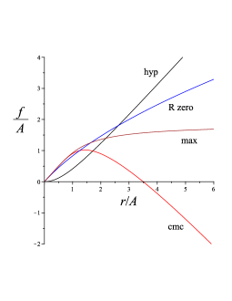
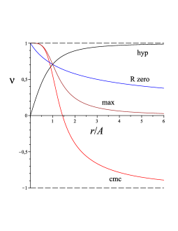
Figure 1: Minkowski spacetime. The radial behavior of the slicing function $f(r)$ (rescaled by $A$) and the associated spatial velocity $\nu=f_{r}$ of observers normal to the slicing itself relative to the observers following the coordinate time lines are shown as functions of $r/A$ in all cases discussed in the text: CMC, maximal, vanishing Ricci scalar and hyperboloidal slicings. The curve corresponding to the CMC slicing is drawn here for $k=1$; as $k$ approaches $0$, this curve approaches the maximal slicing curve more and more. Note that although all these slicings have observer world lines which are initially radially outgoing at the origin of spatial coordinates, the CMC observers reverse direction to become radually ingoing. Only the hyperboloidal slicing is regular at the origin, while the remaining hypersurfaces have an asymptotically null conical singularity there. Reversing the sign of $f(r)$ simply interchanges ingoing and outgoing directions for the relative motion of the new observers with respect to the inertial observers of the rest system.

4 Schwarzschild spacetime

Consider now the Schwarzschild spacetime representing a nonrotating black hole, whose line element written in standard coordinates $(t,r,\theta,\phi)$ is given by

$${\rm d}s^{2} = -\left(1-\frac{2M}{r}\right){\rm d}t^{2}+\left(1-\frac{2M}{r}\right)^{-1}{\rm d}r^{2}+r^{2}({\rm d}\theta^{2}+\sin^{2}\theta\,{\rm d}\phi^{2})\,.$$ (62)

Introduce an orthonormal frame adapted to the static observers following the time lines, i.e.,

$$n=N^{-1}\partial_{t}\,,\qquad e_{\hat{r}}=N\partial_{r}\,,\qquad e_{\hat{\theta}}=\frac{1}{r}\partial_{\theta}\,,\qquad e_{\hat{\phi}}=\frac{1}{r\sin\theta}\partial_{\phi}\,,$$ (63)

with dual frame

$$n^{\flat}=-N{\rm d}t\ ,\quad\omega^{{\hat{r}}}=N^{-1}{\rm d}r\ ,\quad\omega^{{\hat{\theta}}}=r\,{\rm d}\theta\ ,\quad\omega^{{\hat{\phi}}}=r\sin\theta\,{\rm d}\phi\ ,$$ (64)

where $N=\sqrt{1-2M/r}$.

The $t=const$ hypersurfaces form a slicing which is extrinsically flat (as the orthogonal hypersurfaces to the static Killing vector congruence $\partial_{t}$), but not intrinsically flat. The induced metric on these hypersufaces

$${}^{(3)}\kern-1.5pt{\rm d}s^{2}=\left(1-\frac{2M}{r}\right)^{-1}{\rm d}r^{2}+r^{2}({\rm d}\theta^{2}+\sin^{2}\theta{\rm d}\phi^{2})$$ (65)

has nonzero Ricci curvature

$$(R(h)^{a}{}_{b})=\frac{M}{r^{3}}\,{\rm diag}\left(-2,1,1\right)\,,$$ (66)

with vanishing Ricci scalar $R(h)=0$.

Let us look for general slicings of the Schwarzschild geometry which are compatible with the Killing symmetries of the spacetime, i.e., spherical slices $T=t+f(r)$. Their timelike unit normal is

$${\mathcal{N}}^{\flat}=-L({\rm d}t-f_{r}\,{\rm d}r)\,,\qquad{\mathcal{N}}=\gamma(n+\nu\,e_{\hat{r}})\,,$$ (67)

with relative velocity (see Eq. (19))

$$\nu\equiv\nu^{\hat{r}}=N^{2}f_{r}\,\leftrightarrow\,f_{r}=N^{-2}\nu$$ (68)

and associated Lorentz factor $\gamma=1/\sqrt{1-\nu^{2}}$. As in the Minkowski spacetime case, reversing the sign of $f(r)$ interchanges the ingoing and outgoing radially moving observers associated with the new slicing.

The induced metric on $\Sigma$ is

$$(h_{ab})={\rm diag}\left((\gamma N)^{-2},g_{\theta\theta},g_{\phi\phi}\right)\,,$$ (69)

and the new lapse function and shift vector field are

$$L=N\gamma\,,\quad L_{a}=-\nu\delta^{1}{}_{a}\,,\quad L^{a}=-\gamma^{2}N^{2}\nu\,\delta^{a}{}_{1}\,.$$ (70)

A (nonorthonormal) basis on $\Sigma$ is given by

$$E_{1}=\partial_{r}+f_{r}\partial_{t}\,,\quad E_{2}=\partial_{\theta}\,,\quad E_{3}=\partial_{\phi}\,,$$ (71)

with dual frame

$$\Omega^{1}=N\gamma^{2}[\nu\,n^{\flat}+\omega^{\hat{r}}]\,,\quad\Omega^{2}=\frac{1}{\sqrt{g_{\theta\theta}}}\omega^{\hat{\theta}}={\rm d}\theta\,,\quad\Omega^{3}=\frac{1}{\sqrt{g_{\phi\phi}}}\omega^{\hat{\phi}}={\rm d}\phi\,.$$ (72)

The acceleration $a(\mathcal{N})$ is given by

$$a(\mathcal{N})=\frac{1}{N\gamma}\partial_{r}(N\gamma)\,\Omega^{1}\,,$$ (73)

and the extrinsic curvature of the $T=const$ slices then turns out to be

$$K(\mathcal{N})=-\frac{\partial_{r}X}{N^{2}\gamma^{2}}\,\Omega^{1}\otimes\Omega^{1}-rX\left[\Omega^{2}\otimes\Omega^{2}+\sin^{2}\theta\,\Omega^{3}\otimes\Omega^{3}\right]\,,$$ (74)

where $X=N\gamma\nu$, and the traces of its powers then have the following values

$${\rm Tr}[K(\mathcal{N})^{n}]=(-1)^{n}\left[(\partial_{r}X)^{n}+\frac{2}{r^{n}}X^{n}\right]\,,\quad(n=1,2,3)\,.$$ (75)

The intrinsic curvature is described by the following nonvanishing components of the spatial Riemann tensor

$$R(h)_{r\theta r\theta}=\frac{R(h)_{r\phi r\phi}}{\sin^{2}\theta}=-\frac{r}{N\gamma}\partial_{r}(N\gamma)\,,\quad R(h)_{\theta\phi\theta\phi}=r^{2}\sin^{2}\theta\,(1-\gamma^{2}N^{2})\,,$$ (76)

or equivalently by the spatial Ricci tensor, whose nonzero components are

$$R(h)^{r}{}_{r}=-\frac{2}{r}N\gamma\partial_{r}(N\gamma)\,,\quad R(h)^{\theta}{}_{\theta}=R(h)^{\phi}{}_{\phi}=\frac{1}{2}R(h)^{r}{}_{r}+\frac{1}{r^{2}}(1-\gamma^{2}N^{2})\,.$$ (77)

Finally, the spatial Ricci scalar is

$$R(h)=\frac{2}{r^{2}}\partial_{r}\left[r(1-\gamma^{2}N^{2})\right]\,,$$ (78)

showing that $r(1-\gamma^{2}N^{2})=const$ corresponds to vanishing spatial scalar curvature, but $\gamma N=1$ to vanishing spatial curvature.

The Cotton-York tensor (24) vanishes identically, so that spherical slicings are automatically conformally flat.

Geodesic slicings correspond to a spatially constant lapse function $L=N\gamma=L_{0}$, as from Eq. (73). In this case

$$\gamma=\frac{L_{0}}{N}\,,\qquad\nu=\pm\frac{1}{L_{0}}\sqrt{L_{0}^{2}-N^{2}}\,,$$ (79)

and the only surviving component of the spatial Riemann tensor is

$$R(h)_{\theta\phi\theta\phi}=r^{2}\sin^{2}\theta\,(1-L_{0}^{2})\,,$$ (80)

whereas the spatial Ricci tensor is fully specified by

$$R(h)^{\theta}{}_{\theta}=R(h)^{\phi}{}_{\phi}=\frac{1}{r^{2}}(1-L_{0}^{2})\,,$$ (81)

with $R(h)=2(1-L_{0}^{2})/r^{2}$. The value of the parameter $L_{0}$ determines the sign of the intrinsic curvature of the slices, corresponding to either vanishing ($L_{0}=1$), positive ($L_{0}<1$) or negative ($L_{0}>1$) curvature. Note that interpreting $\mathcal{N}$ as the 4-velocity field of a family of (geodesic) test particles, the parameter $L_{0}$ coincides with the (conserved, Killing) energy per unit mass of the particles

$$\tilde{E}=-{\mathcal{N}}_{t}=N\gamma=L_{0}\,.$$ (82)

Therefore, $L_{0}=1$ also represents the case of particles with vanishing radial velocity at spatial infinity; $L_{0}>1$ can be associated with particles starting at infinity with nonzero (inward) velocity; finally, $L_{0}<1$ corresponds to particles starting moving at a finite radial position. In the literature, adapted coordinates to these situations (in the special case of a Schwarzschild spacetime) are referred to as “hail” ($L_{0}>1$), “rain” ($L_{0}=1$) and “drip” ($L_{0}<1$) coordinates (see, e.g., Ref. [2] and references therein).

Let us consider some explicit examples. We will let $C$ denote in each case the dimensionless integration constant appearing in the solution of the ordinary differential equation for the radial velocity $\nu$, all quantities being rescaled by the characteristic length scale of the background curvature (i.e., the mass $M$). For simplicity the solutions for the slicing function $f(r)$ will be given up to an overall sign and the constant of integration will be chosen so that $f(2M)=0$ if this function is finite at $r=2M$, or $\lim_{r\to\infty}f(r)=0$ if it approaches a finite limit at $r\to\infty$, in order to compare the time slices from a common reference point at the horizon or at spatial infinity relative to the usual slicing. Typical behaviors of the slicing functions as well as of the corresponding linear velocities are shown in Fig. 2.

1. CMC:

   Let $M\,{\rm Tr}\,[K(\mathcal{N})]=k=const$. Then using Eq. (75) with $n=0$ one finds

   $$X=-\frac{kr}{3M}+\frac{CM^{2}}{r^{2}}\,,$$ (83)

   formally equivalent to Eq. (45) in the case of a flat spacetime, where $C$ is a dimensionless integration constant, implying that

   $$\nu=\frac{X}{\sqrt{N^{2}+X^{2}}}\,,$$ (84)

   and

   $$h_{rr}=\frac{\nu^{2}}{X^{2}}=(N^{2}+X^{2})^{-1}\,.$$ (85)

   The function $f(r)$ is then given by

   $$f(r)=\int_{2M}^{r}\frac{X}{N^{2}\sqrt{N^{2}+X^{2}}}\,{\rm d}r\,.$$ (86)

   Let $k>0$. Then the radial velocity approaches $\nu\to-1$ for large $r$, independent of the value of $C$. In contrast the behavior at the horizon depends on the sign of the quantity $-8k+3C$. In fact, in the limit $r\to 2M$ one has $\nu\to{\rm sgn}(-8k+3C)$, i.e., $\nu\to 1$ if $C>\frac{8}{3}k$, while $\nu\to-1$ if $C<\frac{8}{3}k$.

2. Maximal:

   For $k=0$ the above relations simplify to

   $$X=\frac{CM^{2}}{r^{2}}\,,$$ (87)

   so that $\nu=CM^{2}{\sqrt{h_{rr}}}/r^{2}$ and

   $$h_{rr}=\left(1-\frac{2M}{r}+\frac{C^{2}M^{4}}{r^{4}}\right)^{-1}\,,$$ (88)

   and

   $$f(r)=-CM^{2}\int_{r}^{\infty}\frac{\sqrt{h_{rr}}}{r^{2}N^{2}}\,{\rm d}r\,,$$ (89)

   which can be expressed in terms of elliptic functions. Therefore the radial velocity behaves as $\nu\to 0$ for large $r$ and $\nu\to 1$ for $r\to 2M$, independent of the value of $C$.

3. Vanishing Ricci curvature:

   Setting $R(h)=0$ in Eq. (78) gives $r(1-\gamma^{2}N^{2})=const$, leading to

   $$\nu=\frac{1}{\sqrt{1+CN^{2}r/M}}\,,$$ (90)

   and

   $$f(r)=\frac{M}{C\nu}(1-\nu)+2M\ln\left(\frac{1-\nu}{1+\nu}\right)\,.$$ (91)

   Therefore the radial velocity behaves as $\nu\to 0$ for large $r$ and $\nu\to 1$ for $r\to 2M$, independent of the value of $C$.

4. Harmonic:

   The harmonic condition (30) gives

   $$0=\partial_{r}\nu+\frac{2\nu}{r}\,,$$ (92)

   so that $\nu=CM^{2}/r^{2}$ and

   $$f(r)=CM\ln N\,.$$ (93)

   $C=4$ is a common choice in the literature. Therefore the radial velocity behaves as $\nu\to 0$ for large $r$ and $\nu\to 1$ for $r\to 2M$ (for that choice of the integration constant).

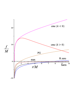
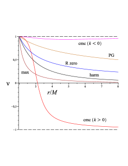
Figure 2: Schwarzschild spacetime. The comparative behavior of the slicing function $f(r)$ (left) and the corresponding radial velocity $\nu$ (right) associated with the special observer families considered in the text (i.e., CMC, maximal, vanishing Ricci scalar, harmonic and PG) is shown for the following choice of parameters: $C=10$, $k=\pm 1$ (CMC); $C=10$ (maximal); $C=1$ (vanishing Ricci scalar); $C=4$ (harm). The outgoing PG slicing ($\nu>0$) is shown to compare with the remaining mostly outgoing radial coordinate associated observers, apart from the positive curvature CMC case which has both radially ingoing and outgoing regimes of their associated observers compared to the usual static observers to which all of these are compared ($\nu=0$). Note that $f$ diverges at radial infinity for the zero curvature, PG, and constant mean curvature slicings, and at $r=2M$ for all but the constant mean curvature slicings, while the maximal and harmonic slicings are chosen to vanish at radial infinity.

Let us investigate now spherical slicings characterized by intrinsic flatness, i.e., by the vanishing of the spatial Riemann tensor. Examining Eq. (76) it is sufficient to impose the condition

$$L=1\leftrightarrow\gamma=\frac{1}{N}\,,\qquad\nu=\pm\sqrt{1-N^{2}}\,,$$ (94)

which obviously yields a flat induced metric apparent from Eq. (69) since $h_{rr}=1$, while similarly the acceleration vanishes as well from Eq. (73), leading to a geodesically parallel slicing. Because of the above choice of the lapse function, the slicing is associated with the “rain” coordinates introduced above, whose adapted observers are known as Painlevé-Gullstrand (PG) observers [3, 4]. They are geodesic and irrotational, and admit orthogonal time hypersurfaces which are intrinsically flat. Their radial velocity relative to the static observers is $\nu=-\sqrt{1-N^{2}}=-\sqrt{2M/r}$, having selected the minus sign corresponding to a free fall from rest at infinity (ingoing PG, for example). Integrating Eq. (68) then gives

$$f(r)=-2\sqrt{2Mr}+2M\ln\frac{\sqrt{r}+\sqrt{2M}}{\sqrt{r}-\sqrt{2M}}\,.$$ (95)

However, PG slicings are not extrinsically flat since

$$M\,K(\mathcal{N})=\sqrt{\frac{2M^{3}}{r^{3}}}\left[\frac{1}{2}\Omega^{1}\otimes\Omega^{1}-r^{2}\,\Omega^{2}\otimes\Omega^{2}-r^{2}\sin^{2}\theta\,\Omega^{3}\otimes\Omega^{3}\right]\,.$$ (96)

PG observers are in a sense “complementary” to the static observers, which instead have extrinsically flat orthogonal time hypersurfaces.

5 Splitting of the curvature tensor by a generic family of observers

For rotating black holes, the situation is more complicated, so we examine first the splitting of the curvature tensor using the test observer congruence associated with a given stationary spacelike slicing. Let $U$ be the unit timelike $4$-velocity vector tangent to the test observer world lines orthogonal to the slicing. The orthogonal decomposition of the covariant derivative of this irrotational congruence $U$ is

$$\nabla_{\alpha}U^{\beta}=-U_{\alpha}a(U)^{\beta}-\theta(U)^{\beta}{}_{\alpha}\,,$$ (97)

where $a(U)^{\beta}=U^{\alpha}\nabla_{\alpha}U^{\beta}$ is the acceleration and

$$\theta(U)_{\alpha\beta}=P(U)^{\mu}_{\alpha}P(U)^{\nu}_{\beta}\nabla_{(\mu}U_{\nu)}$$ (98)

is the expansion tensor with trace $\Theta(U)=\theta(U)^{\alpha}{}_{\alpha}$, the expansion scalar usually referred to as just the expansion of the congruence, while the tracefree part of the expansion tensor $\sigma(U)_{\alpha\beta}$ describes the shear of the congruence.

Details of the decomposition of the curvature tensor and corresponding Einstein equations may be found in many places, including Ref. [24]. Using an observer-adapted frame, the latter lead to the following set of equations in vacuum, setting the Ricci tensor to zero

$$0 = R^{\top}{}_{\top}=[\nabla(U)_{c}+a(U)_{c}]a(U)^{c}-\nabla(U)_{\rm(lie)}\Theta(U)-{\rm Tr}\,[\theta(U)^{2}]\,,$$

$$0 = R^{\top}{}_{a}=-\nabla(U)_{c}[\theta(U)^{c}{}_{a}-\Theta(U)\delta^{c}{}_{a}]\,,$$

$$0 = R^{a}{}_{b}=-[\nabla(U)_{\rm(lie)}+\Theta(U)]\theta(U)^{a}{}_{b}-[\nabla(U)_{(b}+a(U)_{(b}]a(U)^{a)}+R(U){}^{a}{}_{b}\,,$$ (99)

where the index $\top$ corresponds to the component tangential to the congruence $U$ (and proportional to the orthonormal temporal component). Here $\nabla(U)=P(U)\nabla$ and $\nabla(U)_{\rm(lie)}=P(U)\pounds_{U}$ denote the spatial covariant derivative and the spatial Lie derivative, respectively.

Introducing the spatial symmetric “strain” tensor [28, 29, 30, 31, 32],

$$S(U)_{ab}=[\nabla(U)_{(b}+a(U)_{(b}]a(U)_{a)}\,,$$ (100)

these equations can be written

$$\nabla(U)_{\rm(lie)}\Theta(U)={\rm Tr}\,[S(U)]-{\rm Tr}[\theta(U)^{2}]\,,$$ (101)

$$\nabla(U)_{a}[\theta(U)^{a}{}_{c}-\Theta(U)\delta^{a}{}_{c}]=0\,,$$

$$R(U){}^{a}{}_{b}=[\nabla(U)_{\rm(lie)}+\Theta(U)]\theta(U)^{a}{}_{b}+S(U)^{a}{}_{b}\,,$$

If $U$ is a geodesic congruence (i.e., $a(U)=0$), the strain tensor then vanishes identically and Eq. (101) reduces to

$$\nabla(U)_{\rm(lie)}\Theta(U)=-{\rm Tr}[\theta(U)^{2}]\,,$$

$$\nabla(U)_{a}[\theta(U)^{a}{}_{c}-\Theta(U)\delta^{a}{}_{c}]=0\,,$$

$$R(U){}^{a}{}_{b}=[\nabla(U)_{\rm(lie)}+\Theta(U)]\theta(U)^{a}{}_{b}\,.$$ (102)

Therefore in vacuum for irrotational geodesic slicings one has the general result that a nonzero extrinsic curvature implies a nonzero spatial Ricci curvature. This is exactly what happens in the Kerr case when considering Painlevé-Gullstrand observers. What is really special in the Schwarzschild case, instead, is that the extrinsic curvature associated with Painlevé-Gullstrand slicings is nonzero but

$$[\nabla(U)_{\rm(lie)}+\Theta(U)]\theta(U)^{a}{}_{b}=0\,,$$ (103)

implying that $R(U){}^{a}{}_{b}=0$. We will discuss these as well as other related properties in the next section for a Kerr spacetime.

6 Kerr spacetime

Consider the Kerr spacetime representing a rotating black hole with its line element written in standard Boyer-Lindquist coordinates $(t,r,\theta,\phi)$ as

$${\rm d}s^{2}=-\left(1-\frac{2Mr}{\Sigma}\right){\rm d}t^{2}-\frac{4aMr}{\Sigma}\sin^{2}\theta\,{\rm d}t\,{\rm d}\phi+\frac{\Sigma}{\Delta}\,{\rm d}r^{2}+\Sigma\,{\rm d}\theta^{2}+\frac{\Lambda}{\Sigma}\sin^{2}\theta\,{\rm d}\phi^{2}\ ,$$ (104)

where $\Delta=r^{2}-2Mr+a^{2}$, $\Sigma=r^{2}+a^{2}\cos^{2}\theta$ and $\Lambda=(r^{2}+a^{2})^{2}-\Delta a^{2}\sin^{2}\theta$. Here $M$ and $a$ with $|a|\leq M$ are the total mass and the specific angular momentum of the source respectively. The event horizons are located at $r_{\pm}=M\pm\sqrt{M^{2}-a^{2}}$.

The Boyer-Lindquist $t=const$ slicing of the Kerr spacetime is a well known maximal slicing associated with the zero angular momentum observer (ZAMO) family of fiducial observers, with 4-velocity field orthogonal to the slicing leaves given by

$$n^{\flat}=-N{\rm d}t,\qquad n=N^{-1}(\partial_{t}-N^{\phi}\partial_{\phi})\,,$$ (105)

where $N=(-g^{tt})^{-1/2}=\left[\Delta\Sigma/\Lambda\right]^{1/2}$ and $N^{\phi}=g_{t\phi}/g_{\phi\phi}=-2aMr/\Lambda$ are the lapse function and the only nonvanishing component of the shift vector field, respectively, satisfying the relations (useful in manipulating expressions)

$$g_{\phi\phi}N^{2}=\Delta\sin^{2}\theta,\quad\frac{N^{\phi}}{N^{2}}=-\frac{2aMr}{\Delta\Sigma}\ .$$ (106)

An orthonormal frame adapted to the ZAMOs is given by

$$e_{\hat{t}}=n\ ,\quad e_{\hat{r}}=\frac{1}{\sqrt{g_{rr}}}\partial_{r}=\partial_{\hat{r}}\ ,\quad e_{\hat{\theta}}=\frac{1}{\sqrt{g_{\theta\theta}}}\partial_{\theta}=\partial_{\hat{\theta}}\ ,\quad e_{\hat{\phi}}=\frac{1}{\sqrt{g_{\phi\phi}}}\partial_{\phi}=\partial_{\hat{\phi}}\ ,$$ (107)

with dual frame

$$\omega^{{\hat{t}}}=N{\rm d}t\ ,\quad\omega^{{\hat{r}}}=\sqrt{g_{rr}}\,{\rm d}r\ ,\quad\omega^{{\hat{\theta}}}=\sqrt{g_{\theta\theta}}\,{\rm d}\theta\ ,\quad\omega^{{\hat{\phi}}}=\sqrt{g_{\phi\phi}}\,({\rm d}\phi+N^{\phi}{\rm d}t)\ .$$ (108)

The ZAMOs are accelerated and locally nonrotating, and have a nonzero but tracefree expansion tensor completely described in terms of the (shear) expansion vector $\theta(n)_{\hat{\phi}}{}^{\alpha}=\theta(n)^{\alpha}{}_{\beta}\,{e_{\hat{\phi}}}^{\beta}$ as

$$\theta(n)=e_{\hat{\phi}}\otimes\vec{\theta}(n)_{\hat{\phi}}+\vec{\theta}(n)_{\hat{\phi}}\otimes e_{\hat{\phi}}\ .$$ (109)

The extrinsic curvature $K(n)=-\theta(n)$ is nonzero, whereas its trace vanishes making the slicing a maximal one. ${\rm Tr}\,[K(n)^{3}]$ also vanishes, whereas ${\rm Tr}\,[K(n)^{2}]$ is nonzero. In terms of the dimensionless inverse radius $u=M/r$ and the dimensionless rotational parameter $\hat{a}=a/M$, the latter turns out to be

$$M^{2}\,{\rm Tr}\,[K(n)^{2}]=2{\hat{a}}^{2}u^{6}\sin^{2}(\theta)\frac{\alpha\tilde{\Sigma}^{2}-4\beta\tilde{\Sigma}+8u(1+{\hat{a}}^{2}u^{2})}{[\tilde{\Sigma}\tilde{\Delta}+2u(1+{\hat{a}}^{2}u^{2})]^{2}\tilde{\Sigma}^{3}}\,,$$ (110)

with

$$\alpha=-3+8u-6{\hat{a}}^{2}u^{2}+{\hat{a}}^{4}u^{4}\,,\qquad\beta=-3+4u-3{\hat{a}}^{2}u^{2}+2{\hat{a}}^{2}u^{3}\,,$$ (111)

and

$$\tilde{\Sigma}=1+\hat{a}^{2}u^{2}\cos^{2}\theta\,,\qquad\tilde{\Delta}=1-2u+\hat{a}^{2}u^{2}\,.$$ (112)

In the weak field limit $u\ll 1$ the previous expression becomes

$$M^{2}\,{\rm Tr}\,[K(n)^{2}]=18\sin^{2}\theta\,\hat{a}^{2}u^{6}\left[1-\frac{1}{3}(4+13\cos^{2}\theta)\hat{a}^{2}u^{2}\right]+O(u^{10})\,.$$ (113)

Similarly, the intrinsic curvature of the Boyer-Lindquist time coordinate slices is nonzero. In fact, the spatial Ricci tensor has the approximated expression

$$M^{2}\,\,(R(h)^{a}{}_{b}) = u^{3}\begin{pmatrix}-2&0&0\cr 0&1&0\cr 0&0&1\end{pmatrix}+9\hat{a}^{2}\cos\theta\sin\theta\,u^{4}\begin{pmatrix}0&1&0\cr 0&0&0\cr 0&0&0\end{pmatrix}$$ (114)

$$+ 3\hat{a}^{2}u^{5}\begin{pmatrix}5\cos^{2}(\theta)-1&-6\cos\theta\sin\theta&0\cr 0&1-3\cos^{2}\theta&0\cr 0&0&-2\cos^{2}\theta\end{pmatrix}+O(u^{6})\,.$$

The three matrices appearing here have zero trace and only at the next order $u^{6}$ do nonzero trace terms appear. In fact, $M^{2}\,R(h)=M^{2}\,{\rm Tr}\,[K(n)^{2}]$, which results from combining the first and the third of the general relations (101) when $\Theta(U)=0$, and since $M^{2}\,{\rm Tr}\,[K(n)^{2}]$ starts as $O(u^{6})$ in its asymptotic expansion (see Eq. (113)).

The ZAMO kinematical quantities only have nonzero components in the $r$-$\theta$ plane of the tangent space, i.e.

$$a(n) = a(n)^{\hat{r}}\,e_{\hat{r}}+a(n)^{\hat{\theta}}\,e_{\hat{\theta}}=\nabla(n)\ln N\,,$$

$$\vec{\theta}(n)_{\hat{\phi}} = \theta(n)_{\hat{\phi}}{}^{\hat{r}}\,e_{\hat{r}}+\theta(n)_{\hat{\phi}}{}^{\hat{\theta}}\,e_{\hat{\theta}}=-\frac{\sqrt{g_{\phi\phi}}}{2N}\nabla(n)N^{\phi}\,.$$ (115)

For later use it is convenient to introduce the quantity

$$\nu_{n}=\sqrt{g_{\phi\phi}}\,\frac{N^{\phi}}{N}\,,\qquad\gamma_{n}=\frac{N}{\sqrt{-g_{tt}}}\,,$$ (116)

as well as the curvature vectors $k(x^{i},n)$ associated with the diagonal metric coefficients [24, 33, 34, 35]

$$k(x^{i},n)=k(x^{i},n)^{\hat{r}}e_{\hat{r}}+k(x^{i},n)^{\hat{\theta}}e_{\hat{\theta}}=-\nabla(n)\ln\sqrt{g_{ii}}\,.$$ (117)

The relevant ZAMO kinematical quantities are listed in Appendix A. A recent review of ZAMO slicings can be found in Ref. [36].

Let us focus on axisymmetric slices $f=f(r,\theta)$, because the Kerr metric is axially symmetric. The timelike unit normal to these slices is given by

$${\mathcal{N}}^{\flat}=-L({\rm d}t+f_{r}{\rm d}r+f_{\theta}{\rm d}\theta)\,,\qquad{\mathcal{N}}=\gamma(n+\nu^{\hat{r}}e_{\hat{r}}+\nu^{\hat{\theta}}e_{\hat{\theta}})\,,$$ (118)

with relative velocity components and associated Lorentz factor

$$\nu_{\hat{a}}=\frac{N}{\sqrt{g_{aa}}}f_{a}\ ,\qquad\gamma=(1-\delta^{\hat{a}\hat{b}}\nu_{\hat{a}}\nu_{\hat{b}})^{-1/2}\,.$$ (119)

The induced metric on $\Sigma$ is given by

$$(h_{ab})=\begin{pmatrix}g_{rr}&0&0\cr 0&g_{\theta\theta}&0\cr 0&0&g_{\phi\phi}\cr\end{pmatrix}+g_{t\phi}\begin{pmatrix}0&0&f_{r}\cr 0&0&f_{\theta}\cr f_{r}&f_{\theta}&0\cr\end{pmatrix}+g_{tt}\begin{pmatrix}f_{r}^{2}&f_{r}f_{\theta}&0\cr f_{r}f_{\theta}&f_{\theta}^{2}&0\cr 0&0&0\cr\end{pmatrix}\,,$$ (120)

or explicitly

$$h_{rr} = g_{rr}\left(1-\frac{\nu_{\hat{r}}^{2}}{\gamma_{n}^{2}}\right),\quad h_{\theta\theta}=g_{\theta\theta}\left(1-\frac{\nu_{\hat{\theta}}^{2}}{\gamma_{n}^{2}}\right),\quad h_{\phi\phi}=g_{\phi\phi},$$

$$h_{r\theta} = -\frac{\sqrt{g_{rr}g_{\theta\theta}}}{\gamma_{n}^{2}}\,\nu_{\hat{r}}\nu_{\hat{\theta}},\quad h_{r\phi}=\sqrt{g_{rr}g_{\phi\phi}}\,\nu_{n}\nu_{\hat{r}},\quad h_{\theta\phi}=\sqrt{g_{\theta\theta}g_{\phi\phi}}\,\nu_{n}\nu_{\hat{\theta}}\,.$$ (121)

The new lapse is $L=\gamma N$, since $N^{c}f_{c}=0$, taking into account that $N_{a}=N_{\phi}\delta^{\phi}{}_{a}$, whereas the new shift is specified either by the covariant components

$$L_{1}=g_{tt}f_{r}=-\frac{N\sqrt{g_{rr}}}{\gamma_{n}^{2}}\nu_{\hat{r}}\,,\quad L_{2}=g_{tt}f_{\theta}=-\frac{N\sqrt{g_{\theta\theta}}}{\gamma_{n}^{2}}\nu_{\hat{\theta}}\,,\quad L_{3}=g_{t\phi}\equiv N_{\phi}\,,$$ (122)

or the contravariant components

$$L^{1} = -\gamma^{2}N\frac{\nu_{\hat{r}}}{\sqrt{g_{rr}}}\,,\quad L^{2}=-\gamma^{2}N\frac{\nu_{\hat{\theta}}}{\sqrt{g_{\theta\theta}}}\,,\quad L^{3}=\gamma^{2}N^{\phi}\,.$$ (123)

Finally one can evaluate the (nonorthogonal) basis $E_{c}$ and its dual frame $\Omega^{c}$ using Eqs. (123), i.e.,

$$E_{1}=\partial_{r}+f_{r}\partial_{t},\quad E_{2}=\partial_{\theta}+f_{\theta}\partial_{t},\quad E_{3}=\partial_{\phi}\,,$$ (124)

and

$$\Omega^{1}={\rm d}r+\frac{\gamma\nu_{\hat{r}}}{\sqrt{g_{rr}}}\,{\mathcal{N}}^{\flat},\quad\Omega^{2}={\rm d}\theta+\frac{\gamma\nu_{\hat{\theta}}}{\sqrt{g_{\theta\theta}}}\,{\mathcal{N}}^{\flat},\quad\Omega^{3}={\rm d}\phi-\frac{\gamma\nu_{n}}{\sqrt{g_{\phi\phi}}}\,{\mathcal{N}}^{\flat}\,.$$ (125)

Having written the new spatial metric and the normal congruence ${\mathcal{N}}$, obtaining both the kinematical quantities of ${\mathcal{N}}$ as well as the extrinsic and intrinsic curvature of the slice $\Sigma$ is now straightforward. The 4-acceleration $a({\mathcal{N}})=\nabla_{\mathcal{N}}{\mathcal{N}}$ turns out to be

$$a({\mathcal{N}})=a({\mathcal{N}})_{1}\Omega^{1}+a({\mathcal{N}})_{2}\Omega^{2}\,,$$ (126)

with

$$a({\mathcal{N}})_{1} = \sqrt{g_{rr}}(\partial_{\hat{r}}\ln L)=\sqrt{g_{rr}}\left[a(n)_{\hat{r}}+\gamma^{2}(\nu_{\hat{r}}\partial_{\hat{r}}\nu_{\hat{r}}+\nu_{\hat{\theta}}\partial_{\hat{r}}\nu_{\hat{\theta}})\right]\,,$$

$$a({\mathcal{N}})_{2} = \sqrt{g_{\theta\theta}}(\partial_{\hat{\theta}}\ln L)=\sqrt{g_{\theta\theta}}\left[a(n)_{\hat{\theta}}+\gamma^{2}(\nu_{\hat{r}}\partial_{\hat{\theta}}\nu_{\hat{r}}+\nu_{\hat{\theta}}\partial_{\hat{\theta}}\nu_{\hat{\theta}})\right]\,.$$ (127)

With respect to the spatial frame $\{E_{a}\}$, the components of the extrinsic curvature tensor $K(\mathcal{N})=K(\mathcal{N})_{ab}\Omega^{a}\otimes\Omega^{b}$ are given by

$$K(\mathcal{N})_{11} = g_{rr}\gamma\left[\nu_{\hat{r}}(W_{\hat{r}}-2\nu_{n}Z_{\hat{r}})+\nu_{\hat{r}|\hat{r}}\right]\,,$$

$$K(\mathcal{N})_{12} = -\sqrt{g_{rr}g_{\theta\theta}}\gamma\left[\nu_{\hat{r}}(W_{\hat{\theta}}-\nu_{n}Z_{\hat{\theta}})-\nu_{\hat{\theta}}\nu_{n}Z_{\hat{r}}+\nu_{\hat{\theta}|\hat{r}}\right]\,,$$

$$K(\mathcal{N})_{13} = \sqrt{g_{rr}g_{\phi\phi}}\gamma Z_{\hat{r}}\,,$$

$$K(\mathcal{N})_{22} = g_{\theta\theta}\gamma\left[\nu_{\hat{\theta}}(W_{\hat{\theta}}-2\nu_{n}Z_{\hat{\theta}})+\nu_{\hat{\theta}|\hat{\theta}}\right]\,,$$

$$K(\mathcal{N})_{23} = \sqrt{g_{\theta\theta}g_{\phi\phi}}\gamma Z_{\hat{\theta}}\,,$$

$$K(\mathcal{N})_{33} = -g_{\phi\phi}\gamma\nu_{\hat{\phi}|\hat{\phi}}\,,$$ (128)

where

$$Z_{\hat{a}} = \nu_{\hat{a}}\nu_{n}(k(\phi,n)\cdot\nu)-[\theta(n)_{\hat{\phi}}{}_{\hat{a}}-(\theta(n)_{\hat{\phi}}\cdot\nu)\nu_{\hat{a}}]\,,$$

$$W_{\hat{a}} = \nu_{\hat{a}}\nu_{n}^{2}(k(\phi,n)\cdot\nu)+[a(n)_{\hat{a}}-(a(n)\cdot\nu)\nu_{\hat{a}}]\,,$$ (129)

and $\nu_{\hat{a}|\hat{b}}=P(n)^{\alpha}{}_{\hat{a}}P(n)^{\beta}{}_{\hat{b}}\nabla_{\beta}\nu_{\alpha}$, i.e.,

$$\nu_{\hat{r}|\hat{r}} = \partial_{\hat{r}}\nu_{\hat{r}}-k(r,n)_{\hat{\theta}}\nu_{\hat{\theta}}\,,\qquad\nu_{\hat{r}|\hat{\theta}}=\partial_{\hat{\theta}}\nu_{\hat{r}}+k(\theta,n)_{\hat{r}}\nu_{\hat{\theta}}\,,$$

$$\nu_{\hat{\theta}|\hat{r}} = \partial_{\hat{r}}\nu_{\hat{\theta}}+k(r,n)_{\hat{\theta}}\nu_{\hat{r}}\,,\qquad\nu_{\hat{\theta}|\hat{\theta}}=\partial_{\hat{\theta}}\nu_{\hat{\theta}}-k(\theta,n)_{\hat{r}}\nu_{\hat{r}}\,,$$

$$\nu_{\hat{\phi}|\hat{\phi}} = -k(\phi,n)\cdot\nu\,.$$ (130)

The trace then turns out to be

$${\rm Tr}\,[K(\mathcal{N})] = -\gamma\left\{\nu_{\hat{\theta}|\hat{\theta}}+\frac{\nu_{\hat{\phi}|\hat{\phi}}}{\gamma_{n}^{2}}+\gamma^{2}\left[\nu_{\hat{r}|\hat{r}}+\nu_{n}^{2}\nu_{\hat{\phi}|\hat{\phi}}+\nu_{\hat{r}}W_{\hat{r}}+\nu_{\hat{\theta}}W_{\hat{\theta}}\right.\right.$$ (131)

$$\left.\left.+(\nu_{\hat{r}|\hat{\theta}}+\nu_{\hat{\theta}|\hat{r}})\nu_{\hat{r}}\nu_{\hat{\theta}}+(\nu_{\hat{\theta}|\hat{\theta}}-\nu_{\hat{r}|\hat{r}})\nu_{\hat{\theta}}^{2}\right]\right\}\,.$$

The intrinsic curvature associated with the induced metric on $\Sigma$ can be easily calculated too. The nonvanishing components of the spatial Riemann tensor are given by

$$R(\mathcal{N})_{r\phi r\phi} = g_{rr}g_{\phi\phi}[-E(n)_{\hat{\theta}\hat{\theta}}+E(n)_{\hat{\phi}\hat{\phi}}\nu_{\hat{r}}^{2}]+K(\mathcal{N})_{11}K(\mathcal{N})_{33}+[K(\mathcal{N})_{13}]^{2}\,,$$

$$R(\mathcal{N})_{r\phi\theta\phi} = g_{\phi\phi}\sqrt{g_{rr}g_{\theta\theta}}[E(n)_{\hat{r}\hat{\theta}}+E(n)_{\hat{\phi}\hat{\phi}}\nu_{\hat{r}}\nu_{\hat{\theta}}]-K(\mathcal{N})_{12}K(\mathcal{N})_{33}+K(\mathcal{N})_{13}K(\mathcal{N})_{23}\,,$$

$$R(\mathcal{N})_{r\theta r\phi} = g_{rr}\sqrt{g_{\theta\theta}g_{\phi\phi}}[(H(n)_{\hat{r}\hat{r}}+2H(n)_{\hat{r}\hat{\theta}}-\nu_{n}E(n)_{\hat{r}\hat{\theta}})\nu_{\hat{r}}-(H(n)_{\hat{r}\hat{\theta}}-\nu_{n}E(n)_{\hat{\theta}\hat{\theta}})\nu_{\hat{\theta}}]$$

$$+K(\mathcal{N})_{11}K(\mathcal{N})_{23}+K(\mathcal{N})_{12}K(\mathcal{N})_{13}\,,$$

$$R(\mathcal{N})_{r\theta\theta\phi} = g_{\theta\theta}\sqrt{g_{rr}g_{\phi\phi}}[(-H(n)_{\hat{r}\hat{\theta}}+\nu_{n}E(n)_{\hat{r}\hat{r}})\nu_{\hat{r}}+(H(n)_{\hat{\theta}\hat{\theta}}+2H(n)_{\hat{r}\hat{r}}+\nu_{n}E(n)_{\hat{r}\hat{\theta}})\nu_{\hat{\theta}}]$$

$$-K(\mathcal{N})_{12}K(\mathcal{N})_{23}-K(\mathcal{N})_{22}K(\mathcal{N})_{13}\,,$$

$$R(\mathcal{N})_{\theta\phi\theta\phi} = g_{\theta\theta}g_{\phi\phi}[-E(n)_{\hat{r}\hat{r}}+E(n)_{\hat{\phi}\hat{\phi}}\nu_{\hat{\theta}}^{2}]+K(\mathcal{N})_{22}K(\mathcal{N})_{33}+[K(\mathcal{N})_{23}]^{2}\,,$$

$$R(\mathcal{N})_{r\theta r\theta} = g_{rr}g_{\theta\theta}\{-E(n)_{\hat{\phi}\hat{\phi}}+[E(n)_{\hat{\theta}\hat{\theta}}+\nu_{n}(2H(n)_{\hat{r}\hat{\theta}}-\nu_{n}E(n)_{\hat{r}\hat{r}})]\nu_{\hat{r}}^{2}$$ (132)

$$-2[(1+\nu_{n}^{2})E(n)_{\hat{r}\hat{\theta}}+\nu_{n}(H(n)_{\hat{r}\hat{r}}-H(n)_{\hat{\theta}\hat{\theta}})]\nu_{\hat{r}}\nu_{\hat{\theta}}$$

$$+[E(n)_{\hat{r}\hat{r}}-\nu_{n}(2H(n)_{\hat{r}\hat{\theta}}+\nu_{n}E(n)_{\hat{\theta}\hat{\theta}})]\nu_{\hat{\theta}}^{2}\}$$

$$-K(\mathcal{N})_{11}K(\mathcal{N})_{22}+[K(\mathcal{N})_{12}]^{2}\,,$$

where $E(n)$ and $H(n)$ denote the electric and magnetic parts of the spacetime Riemann tensor as measured by ZAMOs, respectively, defined by

$$E(n)_{\alpha\beta}=R_{\alpha\mu\beta\nu}n^{\mu}n^{\nu}\,,\qquad H(n)_{\alpha\beta}=-[R^{*}]_{\alpha\mu\beta\nu}n^{\mu}n^{\nu}\,.$$ (133)

Their nonvanishing frame components are listed in Appendix A. Note that conformally flat axisymmetric slices do not exist in general, as shown in Refs. [15, 16].

We know of no time slicings which take advantage of the extra freedom to depend on the polar angle $\theta$. All of the interesting slicings known to us fall into the special case of “spherical” slicings where $f=f(r)$ depends only on the Boyer-Lindquist radial coordinate $r$, so that $\nu_{\hat{\theta}}=0$ and ${\mathcal{N}}=\gamma(n+\nu_{\hat{r}}\,\omega^{\hat{r}})$, i.e., it is just a boost of $n$ in the radial direction. Thus the new observers moving orthogonally to the new time slicing follow radial trajectories. The induced metric on $\Sigma$ simplifies to

$$(h_{ab})=\begin{pmatrix}g_{rr}&0&0\cr 0&g_{\theta\theta}&0\cr 0&0&g_{\phi\phi}\cr\end{pmatrix}+g_{t\phi}f_{r}\begin{pmatrix}0&0&1\cr 0&0&0\cr 1&0&0\cr\end{pmatrix}+g_{tt}f_{r}^{2}\begin{pmatrix}1&0&0\cr 0&0&0\cr 0&0&0\cr\end{pmatrix}\,.$$ (134)

The components of the 4-acceleration of observers having world lines orthogonal to the slices $\Sigma$ become

$$a({\mathcal{N}})_{1} = \sqrt{g_{rr}}(\partial_{\hat{r}}\ln L)=\sqrt{g_{rr}}\left[a(n)_{\hat{r}}+\gamma^{2}\nu_{\hat{r}}\partial_{\hat{r}}\nu_{\hat{r}}\right]\,,$$

$$a({\mathcal{N}})_{2} = \sqrt{g_{\theta\theta}}(\partial_{\hat{\theta}}\ln L)=\sqrt{g_{\theta\theta}}\left[a(n)_{\hat{\theta}}+\gamma^{2}\nu_{\hat{r}}\partial_{\hat{\theta}}\nu_{\hat{r}}\right]\,,$$ (135)

while the components of the extrinsic curvature tensor of each slice are

$$K(\mathcal{N})_{11} = g_{rr}\gamma\left[\nu_{\hat{r}}(W_{\hat{r}}-2\nu_{n}Z_{\hat{r}})+\partial_{\hat{r}}\nu_{\hat{r}}\right]\,,$$

$$K(\mathcal{N})_{12} = -\sqrt{g_{rr}g_{\theta\theta}}\gamma\nu_{\hat{r}}\left[a(n)_{\hat{\theta}}+\nu_{n}\theta(n)_{\hat{\phi}}{}_{\hat{\theta}}+k(r,n)_{\hat{\theta}}\right]\,,$$

$$K(\mathcal{N})_{13} = \sqrt{g_{rr}g_{\phi\phi}}\gamma Z_{\hat{r}}\,,$$

$$K(\mathcal{N})_{22} = g_{\theta\theta}\gamma\nu_{\hat{r}}k(\theta,n)_{\hat{r}}\,,$$

$$K(\mathcal{N})_{23} = \sqrt{g_{\theta\theta}g_{\phi\phi}}\gamma\theta(n)_{\hat{\phi}}{}_{\hat{\theta}}\,,$$

$$K(\mathcal{N})_{33} = g_{\phi\phi}\gamma\nu_{\hat{r}}k(\phi,n)_{\hat{r}}\,,$$ (136)

with

$${\rm Tr}\,[K(\mathcal{N})]=-\gamma\left[\gamma^{2}\partial_{\hat{r}}\nu_{\hat{r}}+(a(n)_{\hat{r}}-k(\theta,n)_{\hat{r}}-k(\phi,n)_{\hat{r}})\nu_{\hat{r}}\right]\,.$$ (137)

Finally, the nonvanishing components of the spatial Riemann tensor (6) simplify to

$$R(\mathcal{N})_{r\phi r\phi} = g_{rr}g_{\phi\phi}[-E(n)_{\hat{\theta}\hat{\theta}}+E(n)_{\hat{\phi}\hat{\phi}}\nu_{\hat{r}}^{2}]+K(\mathcal{N})_{11}K(\mathcal{N})_{33}+[K(\mathcal{N})_{13}]^{2}\,,$$

$$R(\mathcal{N})_{r\phi\theta\phi} = g_{\phi\phi}\sqrt{g_{rr}g_{\theta\theta}}\,E(n)_{\hat{r}\hat{\theta}}-K(\mathcal{N})_{12}K(\mathcal{N})_{33}+K(\mathcal{N})_{13}K(\mathcal{N})_{23}\,,$$

$$R(\mathcal{N})_{r\theta r\phi} = g_{rr}\sqrt{g_{\theta\theta}g_{\phi\phi}}\,[H(n)_{\hat{r}\hat{r}}+2H(n)_{\hat{r}\hat{\theta}}-\nu_{n}E(n)_{\hat{r}\hat{\theta}}]\nu_{\hat{r}}$$

$$+K(\mathcal{N})_{11}K(\mathcal{N})_{23}+K(\mathcal{N})_{12}K(\mathcal{N})_{13}\,,$$

$$R(\mathcal{N})_{r\theta\theta\phi} = g_{\theta\theta}\sqrt{g_{rr}g_{\phi\phi}}\,[-H(n)_{\hat{r}\hat{\theta}}+\nu_{n}E(n)_{\hat{r}\hat{r}}]\nu_{\hat{r}}$$

$$-K(\mathcal{N})_{12}K(\mathcal{N})_{23}-K(\mathcal{N})_{22}K(\mathcal{N})_{13}\,,$$

$$R(\mathcal{N})_{\theta\phi\theta\phi} = -g_{\theta\theta}g_{\phi\phi}E(n)_{\hat{r}\hat{r}}+K(\mathcal{N})_{22}K(\mathcal{N})_{33}+[K(\mathcal{N})_{23}]^{2}\,,$$

$$R(\mathcal{N})_{r\theta r\theta} = g_{rr}g_{\theta\theta}\{-E(n)_{\hat{\phi}\hat{\phi}}+[E(n)_{\hat{\theta}\hat{\theta}}+\nu_{n}(2H(n)_{\hat{r}\hat{\theta}}-\nu_{n}E(n)_{\hat{r}\hat{r}})]\nu_{\hat{r}}^{2}\}$$ (138)

$$-K(\mathcal{N})_{11}K(\mathcal{N})_{22}+[K(\mathcal{N})_{12}]^{2}\,.$$

Note that again as in the Schwarzschild case, geodesic slicings correspond to spatially constant lapse function $L=L_{0}$, and one could in principle consider the analogous hail, rain and drip coordinate systems. However, in this case the simple geometrical properties of the intrinsic curvature are lost, and we will limit our discussion (see below) to the case of rain observers ($L_{0}=1$), which are identified with PG observers.

Next some explicit examples are considered. The behavior of the associated linear velocities is shown in Fig. 3.

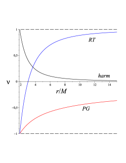
Figure 3: Kerr spacetime slicings. The behavior of the linear velocities associated with the special observer families considered in the text (i.e., harmonic, PG and RT) is shown for the choice of parameters $a/M=0.5$ and $\theta=\pi/2$, for which the outer horizon is located at $r_{+}\approx 1.867M$.

6.1 Harmonic slicings

The harmonic condition (30) implies

$$\partial_{\hat{r}}\nu_{\hat{r}}=[k(\theta,n)_{\hat{r}}+k(\phi,n)_{\hat{r}}]\nu_{\hat{r}}\,,$$ (139)

so that

$$\nu_{\hat{r}}=\frac{C\sin\theta}{\sqrt{g_{\theta\theta}g_{\phi\phi}}}\,,$$ (140)

or equivalently

$$f_{r}=\frac{C}{\Delta}\,.$$ (141)

Further integrating then gives

$$f(r)=\frac{C}{r_{+}-r_{-}}\ln\left|\frac{r-r_{+}}{r-r_{-}}\right|\,,$$ (142)

Regularity of the new lapse function then requires $C=r_{+}^{2}+a^{2}$.

Harmonic slicings are neither intrinsically nor extrinsically flat. For example, the Ricci scalar has the following approximate expression

$$M^{2}\,R(h)=4{\hat{a}}^{2}u^{4}[\cos^{2}\theta+(3\cos^{2}\theta-1)u]+O(u^{6})\,.$$ (143)

The traces (linear, quadratic, cubic) of the extrinsic curvature associated with harmonic observers are shown in Fig. 4.

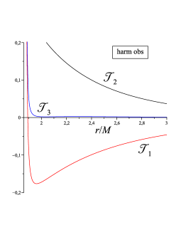
Figure 4: Kerr spacetime, harmonic observers. The traces (linear, quadratic and cubic) of the extrinsic curvature associated with harmonic observers are shown for the same choice of parameters as in Fig. 3.

6.2 Geodesic slicings

Geodesic slicings are characterized by vanishing acceleration, i.e., by constant lapse function $L=L_{0}$ of the spacetime metric written in adapted coordinates. Therefore, they are identified by the condition

$$\gamma=\frac{L_{0}}{N}\,,\qquad\nu_{\hat{r}}=\pm\sqrt{L_{0}^{2}-N^{2}}\,,$$ (144)

the same condition as in the corresponding Schwarzschild spacetime.

When $L_{0}=1$ these slicings are associated with the PG observers, whose world lines are a timelike congruence with both vanishing acceleration and vorticity in the Kerr spacetime as well [3, 4, 14, 37, 38, 39]. Their relative velocity with respect to the ZAMOs is

$$\nu_{\hat{r}}=-\sqrt{1-N^{2}}=-\sqrt{\frac{2Mr(r^{2}+a^{2})}{\Sigma g_{\phi\phi}}}\sin\theta\,,$$ (145)

corresponding to radially infalling observers, leading to

$$f(r)=-\int\frac{\sqrt{2Mr(r^{2}+a^{2})}}{\Delta}\,{\rm d}r\,.$$ (146)

In contrast to the Schwarzschild case, the geodesic condition does not imply intrinsic flatness since the Ricci tensor of the induced metric does not vanish identically. It can be expressed in terms of the extrinsic curvature tensor as in Eq. (5). The spatial curvature scalar is given by

$$R(h)=\frac{2a^{2}Mr(3\cos^{2}\theta-1)}{\Sigma^{3}}\,.$$ (147)

Thus the geometry associated with the PG observers in the Kerr spacetime is neither intrinsically nor extrinsically flat.

For completeness we list also the linear, quadratic and cubic invariants of $K({\mathcal{N}}_{\rm PG})$:

$$M\,{\rm Tr}\,[K({\mathcal{N}}_{\rm PG})] = \frac{u^{3/2}}{\tilde{\Sigma}[2(1+\hat{a}^{2}u^{2})]^{1/2}}(3+{\hat{a}}^{2}u^{2})\,,$$

$$M^{2}\,{\rm Tr}\,[K({\mathcal{N}}_{\rm PG})^{2}] = \frac{u^{3}}{2{\tilde{\Sigma}}^{3}(1+\hat{a}^{2}u^{2})}[9+(10-3\cos^{2}\theta){\hat{a}}^{2}u^{2}$$

$$+(5-6\cos^{2}\theta){\hat{a}}^{4}u^{4}+\cos^{2}\theta\,{\hat{a}}^{6}u^{6}]\,,$$

$$M^{3}\,{\rm Tr}\,[K({\mathcal{N}}_{\rm PG})^{3}] = \frac{u^{9/2}}{{\tilde{\Sigma}}^{4}[2(1+\hat{a}^{2}u^{2})]^{3/2}}[15+3(7-\cos^{2}\theta){\hat{a}}^{2}u^{2}$$ (148)

$$+21\sin^{2}\theta{\hat{a}}^{4}u^{4}+(7-9\cos^{2}\theta){\hat{a}}^{6}u^{6}+\cos^{2}\theta\,{\hat{a}}^{8}u^{8}]\,.$$

The eigenvalues of $K({\mathcal{N}}_{\rm PG})$ are also easily evaluated

$$M\lambda_{0} = \frac{\sqrt{2}u^{3/2}}{\tilde{\Sigma}\sqrt{1+\hat{a}^{2}u^{2}}}\,,$$ (149)

$$M\lambda_{\pm} = \frac{M\lambda_{0}}{4}(1+\hat{a}^{2}u^{2})\pm\left(\frac{u}{2{\tilde{\Sigma}}}\right)^{3/2}[9+3(3-5\cos^{2}\theta){\hat{a}}^{2}u^{2}+\cos^{2}\theta\,{\hat{a}}^{4}u^{4}]^{1/2}\,.$$

Note that $\lambda_{0}$ is always positive. In the Schwarzschild limit the above expressions reduce to $M\lambda_{0}=M\lambda_{+}=-2M\lambda_{-}=\sqrt{2}u^{3/2}$. The traces (linear, quadratic, cubic) of the extrinsic curvature associated with PG observers are shown in Fig. 5.

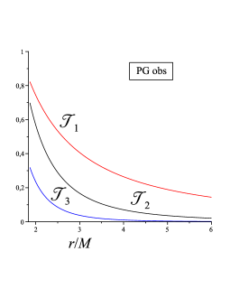
Figure 5: Kerr spacetime, PG observers. The rescaled traces (linear, quadratic and cubic) of the extrinsic curvature associated with the PG observers are shown for the same choice of parameters as in Fig. 3.

6.3 Hyperboloidal slicings

Numerical relativity computations (like those concerning outgoing gravitational radiation) use preferred hyperboloidal spacetime slicings. A general framework for the construction of hyperboloidal coordinates with scri-fixing (i.e., with an explicit prescription to fix the coordinate location of null infinity) for stationary, weakly asymptotically flat spacetimes (including black hole spacetimes) was first developed by Moncrief [40] (see also [41, 42]).

Recently this method has been successfully applied to the numerical investigation of tail decay rates in a Kerr spacetime by Racz and Toth (RT) [43] (see also Refs. [44, 45, 46]). Their construction starts from the standard Boyer-Lindquist coordinates $(t,r,\theta,\phi)$, passing then to ingoing Kerr coordinates $(\bar{t},r,\theta,\bar{\phi})$ such that

$$\bar{t}=t-r+\int\frac{r^{2}+a^{2}}{\Delta}\,{\rm d}r\,,\qquad\bar{\phi}=\phi+\int\frac{a}{\Delta}\,{\rm d}r\,.$$ (150)

Finally, the time and radial coordinates $\bar{t}$ and $r$ are replaced by the new time coordinate $T$ and the compactified radial coordinate $R$, implicitly defined by

$$\bar{t}=T-4M\left[\ln\left(1-\frac{R^{2}}{M^{2}}\right)-\frac{1}{4}\frac{M^{2}+R^{2}}{M^{2}-R^{2}}\right]\,,\qquad r=\frac{2M^{2}R}{M^{2}-R^{2}}\,.$$ (151)

The advantage of using RT coordinates $(T,R,\theta,\bar{\phi})$ is that the time slices are horizon penetrating and connect to future null infinity, so that no boundary conditions are needed. The relation for the radial coordinate $r=r(R)$ can be easily inverted, leading to

$$\frac{R}{M}=\sqrt{1+\frac{M^{2}}{r^{2}}}-\frac{M}{r}\,.$$ (152)

Solving for $T$ then gives $T=t-f(r)$ with

$$f(r)=r-\int\frac{r^{2}+a^{2}}{\Delta}\,{\rm d}r-4M\left[\ln\left(1-\frac{R^{2}}{M^{2}}\right)-\frac{1}{4}\frac{M^{2}+R^{2}}{M^{2}-R^{2}}\right]\,.$$ (153)

RT observers thus form an irrotational congruence ${\mathcal{N}}_{\rm RT}$ of world lines moving radially with respect to ZAMOs, with a relative velocity given by

$$\nu_{\hat{r}}=\frac{N}{\sqrt{g_{rr}}}\left[-\frac{2Mr}{\Delta}+\frac{4M}{r}\left(1+\frac{\frac{1}{4}-\frac{M^{2}}{r^{2}}}{\frac{R}{r}+\frac{M^{2}}{r^{2}}}\right)\right]\,,$$ (154)

with $R=R(r)$ as defined in Eq. (152). It is easy to show also that

$$\lim_{r\to r_{+}}\nu_{\hat{r}}=-1\,,\quad\lim_{r\to\infty}\nu_{\hat{r}}=1\,,$$ (155)

with $\nu_{\hat{r}}$ passing monotonically from $-1$ to $+1$, irrespective of the value of $\theta$ (see Fig. 3).

The traces (linear, quadratic and cubic) of the extrinsic curvature are shown in Fig. 6.

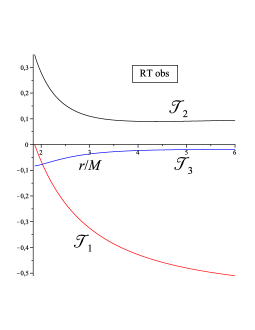
Figure 6: Kerr spacetime, RT observers. The traces (linear, quadratic and cubic) of the extrinsic curvature associated with RT observers are shown for the same choice of parameters as in Fig. 3.

7 Concluding remarks

Special congruences of timelike world lines in Kerr spacetime have been studied extensively in the literature (see, e.g., Refs. [33, 34] and references therein), while in contrast there exist only a few interesting spacetime spacelike slicings that have been investigated. The most natural one is the maximal spacelike slicing associated with the Boyer-Lindquist time coordinate, whose properties are best described in terms of the orthogonal congruence of timelike world lines threading this slicing associated with the so-called ZAMO observers. This congruence is accelerated and shearing but (locally) nonrotating, but the induced metric on the slices does not have any special properties. Nevertheless, other interesting slicings can be found compatible with the Killing symmetries of the spacetime, motivated either by geometrical or analytical considerations.

We have developed here a general framework for analyzing all possible stationary slicings allowed in a given stationary geometry, then specialized our results to black hole spacetimes, reviewing the various familiar examples which can be found in the literature. Geometrical properties of these slicings can be characterized either in terms of those of the kinematical properties of their orthogonal timelike congruences interpreted as the world lines of a family of stationary observers, or in terms of intrinsic or extrinsic curvature properties of the slicing itself. We have considered in detail the case of slicings associated with a new time coordinate function of the Boyer-Lindquist coordinates $(t,r)$. The case of geodesic observers includes the so-called Painlevé-Gullstrand slicing of Kerr. The latter are even more special in the limiting Schwarzschild case where the slices are also intrinsically flat. Finally we have also presented examples of “analytical” slicings of black hole spacetimes, like those associated with harmonic and hyperboloidal time gauges.

Appendix A ZAMO relevant quantities in the Kerr spacetime

We list below the non-vanishing components of the electric and magnetic parts of the Riemann tensor as well as the relevant kinematical quantities as measured by ZAMOs.

The components of the acceleration and expansion vectors are given by

$$a(n)^{\hat{r}} = \frac{M\sin^{2}\theta}{\Sigma^{5/2}\sqrt{\Delta}g_{\phi\phi}}\left\{-2r^{2}(r^{2}+a^{2})\Delta+\Sigma[(r^{2}+a^{2})^{2}-4Mr^{3}]\right\}\,,$$

$$a(n)^{\hat{\theta}} = -\frac{2a^{2}Mr}{\Sigma^{5/2}g_{\phi\phi}}(r^{2}+a^{2})\sin^{3}\theta\cos\theta\,,$$

$$\theta(n)_{\hat{r}\hat{\phi}} = -\frac{Ma\sin^{3}\theta}{\Sigma^{5/2}g_{\phi\phi}}[2r^{2}(r^{2}+a^{2})+\Sigma(r^{2}-a^{2})]\,,$$

$$\theta(n)_{\hat{\theta}\hat{\phi}} = \frac{2a^{3}Mr}{\Sigma^{5/2}g_{\phi\phi}}\sqrt{\Delta}\cos\theta\sin^{4}\theta\,,$$ (156)

and the curvature components are

$$k(r,n)^{\hat{r}} = \frac{\Sigma(r-M)-r\Delta}{\Sigma^{3/2}\sqrt{\Delta}}\,,\qquad k(r,n)^{\hat{\theta}}=\frac{a^{2}\sin\theta\cos\theta}{\Sigma^{3/2}}\,,$$

$$k(\theta,n)^{\hat{r}} = -\frac{r\sqrt{\Delta}}{\Sigma^{3/2}}\,,\qquad k(\theta,n)^{\hat{\theta}}=\frac{a^{2}\sin\theta\cos\theta}{\Sigma^{3/2}}\,,$$

$$k(\phi,n)^{\hat{r}} = \frac{\sqrt{\Delta}\sin^{2}\theta}{\Sigma^{5/2}g_{\phi\phi}}[-\Sigma^{2}(r-M)-M\Sigma(3r^{2}+a^{2})+2Mr^{2}(r^{2}+a^{2})]\,,$$

$$k(\phi,n)^{\hat{\theta}} = -\frac{\cos\theta\sin\theta}{\Sigma^{5/2}g_{\phi\phi}}[\Sigma^{2}\Delta+2Mr(r^{2}+a^{2})^{2}]\,.$$ (157)

Finally, the nontrivial components of the electric and magnetic parts of the Riemann tensor with respect to ZAMOs are given by

$$E_{\hat{r}\hat{r}} = \partial_{\hat{r}}a(n)_{\hat{r}}+a(n)_{\hat{r}}^{2}-3\theta(n)_{\hat{r}\hat{\phi}}^{2}-a(n)_{\hat{\theta}}k(r,n)^{\hat{\theta}}\,,$$

$$E_{\hat{\theta}\hat{\theta}} = -E_{\hat{r}\hat{r}}+\partial_{\hat{r}}k(\theta,n)^{\hat{r}}-[k(\theta,n)^{\hat{r}}]^{2}+\partial_{\hat{\theta}}k(r,n)^{\hat{\theta}}-[k(r,n)^{\hat{\theta}}]^{2}\,,$$

$$E_{\hat{r}\hat{\theta}} = \partial_{\hat{\theta}}a(n)_{\hat{r}}+a(n)_{\hat{\theta}}[a(n)_{\hat{r}}+k(\theta,n)^{\hat{r}}]-3\theta(n)_{\hat{r}\hat{\phi}}\theta(n)_{\hat{\theta}\hat{\phi}}\,,$$

$$H_{\hat{r}\hat{r}} = \partial_{\hat{\theta}}\theta(n)_{\hat{r}\hat{\phi}}-\theta(n)_{\hat{r}\hat{\phi}}k(\phi,n)^{\hat{\theta}}+\theta(n)_{\hat{\theta}\hat{\phi}}[k(\theta,n)^{\hat{r}}-k(\phi,n)^{\hat{r}}]\,,$$

$$H_{\hat{r}\hat{\theta}} = -\partial_{\hat{r}}\theta(n)_{\hat{r}\hat{\phi}}+2\theta(n)_{\hat{r}\hat{\phi}}k(\phi,n)^{\hat{r}}+\theta(n)_{\hat{\theta}\hat{\phi}}k(r,n)^{\hat{\theta}}\,,$$

$$H_{\hat{\phi}\hat{\phi}} = \theta(n)_{\hat{r}\hat{\phi}}[a(n)_{\hat{\theta}}+k(\phi,n)^{\hat{\theta}}]-\theta(n)_{\hat{\theta}\hat{\phi}}[a(n)_{\hat{r}}+k(\phi,n)^{\hat{r}}]\,,$$ (158)

in terms of the above kinematical quantities.

In the equatorial plane, the acceleration and expansion and curvature vectors are all directed along the radial direction, with components

$$a(n)^{\hat{r}}=\frac{M}{r^{2}\sqrt{\Delta}}\frac{(r^{2}+a^{2})^{2}-4a^{2}Mr}{r^{3}+a^{2}r+2a^{2}M}\,,\quad\theta_{\phi}(n)^{\hat{r}}=-\frac{aM(3r^{2}+a^{2})}{r^{2}(r^{3}+a^{2}r+2a^{2}M)}\,,$$ (159)

and

$$\kappa(r,n)^{\hat{r}} = \frac{Mr-a^{2}}{r^{2}\sqrt{\Delta}}\,,\qquad\kappa(\theta,n)^{\hat{r}}=-\frac{\sqrt{\Delta}}{r^{2}}\,,$$

$$k(\phi,n)^{\hat{r}} = -\frac{(r^{3}-a^{2}M)\sqrt{\Delta}}{r^{2}(r^{3}+a^{2}r+2a^{2}M)}\,,$$ (160)

respectively, whereas the nonvanishing frame components (A) of the electric and magnetic parts of the Riemann tensor reduce to

$$E_{\hat{r}\hat{r}} = -\frac{M(2r^{4}+5r^{2}a^{2}-2a^{2}Mr+3a^{4})}{r^{4}(r^{3}+a^{2}r+2a^{2}M)}\,,\quad E_{\hat{\theta}\hat{\theta}}=-E_{\hat{\phi}\hat{\phi}}-E_{\hat{r}\hat{r}}\,,\quad E_{\hat{\phi}\hat{\phi}}=\frac{M}{r^{3}}\,,$$

$$H_{\hat{r}\hat{\theta}} = -\frac{3Ma(r^{2}+a^{2})\sqrt{\Delta}}{r^{4}(r^{3}+a^{2}r+2a^{2}M)}\,.$$ (161)

References

• [1] Taylor E F and Wheeler J A 2000 Exploring Black Holes: Introduction to General Relativity Addison Wesley Longman San Francisco
• [2] Finch T K 2014 Coordinate families for the Schwarzschild geometry based on radial timelike geodesics arxiv: 1211.4337 [gr-qc]
• [3] Painlevé P 1921 C. R. Acad. Sci. (Paris) 173 677
• [4] Gullstrand A 1922 Arkiv. Mat. Astron. Fys. 16 1
• [5] Hamilton A and Lisle J 2008 Am. Jour. Phys. 76, 519
• [6] Smarr L and York J W Jr. 1978 Phys. Rev. D 17 2529
• [7] Malec E and O’Murchadha N 2003 Phys. Rev. D 68 124019
• [8] Malec E and O’Murchadha N 2009 Phys. Rev. D 80 024017
• [9] Schinkel D Macedo R P and Ansorg M 2014 Class. Quant. Grav.  31 075017
• [10] Estabrook F Wahlquist H Christensen S DeWitt B Smarr L and Tsiang E 1973 Phys. Rev. D 7 2814
• [11] Geyer A and Herold H 1995 Phys. Rev. D 52 6182
• [12] Barceló C Liberati S and Visser M 2005 Liv. Rev. Rel. 8 12
• [13] Visser M 2005 Int. J. Mod. Phys. D 14 2051
• [14] Doran C 2000 Phys. Rev. D 61 067503
• [15] Garat A and Price R 2000 Phys. Rev. D 61 124011
• [16] Kroon J 2004 Phys. Rev. Lett. 92 041101
• [17] Bona C and Massó J 1988 Phys. Rev. D 38 8 2419
• [18] Cook G B and Scheel M A 1997 Phys. Rev. D 56 8 4775
• [19] Cook G B 2000 Liv. Rev. Rel. 3 5
• [20] Ohme F Hannam M Husa S and O’Murchadha N 2009 Class. Quant. Grav. 26 175014
• [21] Zenginoglu A and Kidder L E 2010 Phys. Rev. D 81 124010
• [22] Schinkel D Ansorg M and Macedo R P 2014 Class. Quant. Grav.  31 165001
• [23] Misner C W Thorne K S and Wheeler J A 1973 Gravitation Freeman San Francisco
• [24] Jantzen R T Carini P and Bini D 1992 Ann. Phys. (N.Y.) 215 1
• [25] Bini D Jantzen R T and Miniutti G 2001 Class. Quant. Grav. 18 4969
• [26] Bini D Cherubini C Jantzen R T and Miniutti G 2004 Class. Quant. Grav. 21 1987
• [27] Gourgoulhon E 2012 “$3+1$ Formalism in General Relativity,” Lecture Notes in Physics 846
• [28] de Felice F and Usseglio-Tomasset S 1992 Gen. Rel. Grav. 24 1091
• [29] de Felice F and Usseglio-Tomasset S 1993 Class. Quantum Grav. 10 353
• [30] de Felice F and Usseglio-Tomasset S 1996 Gen. Rel. Grav. 28 179
• [31] Bini D de Felice F and Geralico A 2006 Class. Quantum Grav. 23 7603
• [32] Bini D de Felice F and Geralico A 2007 Phys. Rev. D 76 047502
• [33] Bini D Carini P Jantzen R T 1997 Int. J. Mod. Phys. D 6 1
• [34] Bini D Carini P Jantzen R T 1997 Int. J. Mod. Phys. D 6 143
• [35] Bini D de Felice F and Jantzen R T 1999 Class. Quant. Grav. 16 2105
• [36] Frolov A V and Frolov V P 2014 Phys. Rev. D 90 124010
• [37] Natario J 2009 Gen. Rel. Grav. 41 2579
• [38] Herrero A and Morales Lladosa J A 2010 Class. Quant. Grav. 27 175007
• [39] Bini D Geralico A Jantzen R T 2012 Gen. Rel. Grav. 44 603
• [40] Moncrief V 2000 “Conformally regular ADM evolution equations,” Talk at Santa Barbara, http://online.itp.ucsb.edu/online/numrel00/moncrief.
• [41] Zenginoglu A 2008 Class. Quant. Grav.  25 145002
• [42] Zenginoglu A Nunez D and Husa S 2009 Class. Quant. Grav.  26 035009
• [43] Racz I and Toth G Z 2011 Class. Quant. Grav.  28 195003
• [44] Bernuzzi S Nagar A and Zenginoglu A 2011 Phys. Rev. D 84 084026
• [45] Yang H Zimmerman A Zenginoglu A Zhang F Berti E and Chen Y 2013 Phys. Rev. D 88 044047
• [46] Harms E Bernuzzi S Nagar A and Zenginoglu A 2014 Class. Quantum Grav. 31 245004