Recursive multiport schemes for implementing quantum algorithms with photonic integrated circuits

Abstract

We present recursive multiport schemes for implementing quantum Fourier transforms and the inversion step in Grover’s algorithm on an integrated linear optics device. In particular, each scheme shows how to execute a quantum operation on $2d$ modes using a pair of circuits for the same operation on $d$ modes. The circuits operate on path-encoded qudits and realize $d$-dimensional unitary transformations on these states using linear optical networks with $O\left(d^{2}\right)$ optical elements. To evaluate the schemes against realistic errors, we ran simulations of proof-of-principle experiments using a simple fabrication model of silicon-based photonic integrated devices that employ directional couplers and thermo-optic modulators for beam splitters and phase shifters, respectively. We find that high-fidelity performance is achievable with our multiport circuits for $2$-qubit and $3$-qubit quantum Fourier transforms, and for quantum search on four-item and eight-item databases.

I Introduction

Linear optics with single photon sources and detectors provides a promising candidate for establishing efficient and scalable universal quantum computation Knill et al. (2001); Kok et al. (2007). Some specific advantages of optical implementations are the robustness of photons against decoherence and ultrafast optical processing. Meanwhile, current limitations include low efficiencies in photon creation and measurement, and the difficulty of storing photonic quantum information in a quantum memory. However, the main technical challenge with the scalability of linear optical devices is the considerable overhead necessary for realizing multi-qubit gates. Moreover, maintaining phase stability between optical modes often requires active checking and calibration—a task that clearly becomes more demanding the larger the circuit gets. Both of these issues are addressed by integrated photonic technology.

A photonic integrated circuit (PIC) is a multiport device consisting of an integrated system of optical elements embedded onto a single chip using a waveguide architecture Marshall et al. (2009); Thompson et al. (2011). Because PICs are compact and designed to have inherent phase stability, they offer the potential for a truly scalable optical quantum computer. They are also fully compatible with electronic devices and fiber optic systems, which can lead to increased functionality.

There has been much progress made in PIC-based approaches to quantum optics: recent experiments have demonstrated linear optical quantum gates Politi et al. (2008); Laing et al. (2010), multiphoton entanglement Matthews et al. (2009); Shadbolt et al. (2011) boson sampling experiments Aaronson and Arkhipov (2011); Crespi et al. (2013a); Broome et al. (2013), quantum walks in optical arrays Owens et al. (2011); Sansoni et al. (2012); Crespi et al. (2013b), and simulation of quantum systems Lanyon et al. (2010); Aspuru-Guzik and Walther (2012). More generally, PICs offer a natural platform for conducting experiments on quantum systems with higher-dimensional Hilbert spaces Tabia (2012); Schaeff et al. (2015).

In this paper, we describe recursive multiport schemes for carrying out quantum operations on a PIC. By recursive we mean that two copies of the $d$-dimensional circuit are used to construct the $2d$-dimensional version. Formally, a multiport circuit represents a decomposition of a unitary transformation into a network of single-qubit gates acting on adjacent modes, which on a PIC is mapped onto a sequence of beam splitters and phase shifters. It is crucial to note that in our schemes, the photons represent multi-rail qudits, not dual-rail qubits. This is an important distinction since existing methods for performing entangling gates on dual-rail qubits are not very scalable. However, our circuits act on single qudits, therefore, such entangling gates are not needed.

We must emphasize, though, that linear optical implementations on single photonic qudits are inherently unscalable for quantum computation since they require an exponential number of optical modes. The only known way for performing scalable quantum computation with linear optics requires multi-photon quantum interference and and measurement-based nonlinearity, such as in the KLM proposal Knill et al. (2001). Nevertheless, there are several contexts in which our recursive circuits may find suitable application, for instance, within a larger architecture of entangled qudits Joo et al. (2007) or when using QFT as a verification tool in boson sampling Tichy et al. (2014), the latter having been experimentally demonstrated by Carolan, et al. Carolan et al. (2015).

Here, we consider circuits for two important families of unitary transformations: quantum Fourier transform, which is an important subroutine in many quantum algorithms, is covered in Section II, and inversion about the mean, which is a key step for the iterations in Grover’s algorithm, is covered in Section III. In both cases, we provide a recipe for constructing a linear optical network that uses a total of $O\left(d^{2}\right)$ beam splitters and phase shifters for realizing a quantum operation on $d$ modes. The basis for these constructions are efficient matrix factorizations of the $2d$-dimensional unitary operators into a product of a matrix consisting of two copies of a $d$-dimensional version of the same unitary operator and some sparse matrices with $2\times 2$ blocks on the diagonal. Thus, our schemes provide a systematic way of constructing larger circuits from smaller ones, which is quite beneficial for scaling these quantum operations to higher dimensions.

To demonstrate the practical viability of our multiport scheme, we also conducted simulations of experiments on the circuits for quantum Fourier transform and Grover’s algorithm using a fabrication model that incorporates realistic errors in the beam splitters and phase shifters based on wafer-scale testing data on PIC components Mower et al. (2015). The simulation results are discussed in Section IV.

II Quantum Fourier transforms

Many known quantum algorithms that exhibit exponential speedup over their classical counterparts make use of quantum Fourier transform (QFT), which describes a discrete Fourier transform on quantum mechanical amplitudes Nielsen and Chuang (2000). Typically, the speedups come from performing quantum phase estimation, which involves finding approximate eigenvalues of a unitary operator, and it involves an inverse QFT. It is especially helpful in solving interesting problems like prime factorization and discrete logarithms Shor (1997).

There have been some recent experiments that realize QFT with optical multiport circuits, in particular, the four-mode version by Laing et al. Laing et al. (2012), which was performed with path-and-polarization encoded states in bulk optics, and a six-mode version used in the study of inequivalent classes of complex Hadamard matrices by Carolan, et al. Carolan et al. (2015). These examples provide evidence for the considerable interest in developing practical linear optical methods for implementing QFT.

In this section, we describe a recursive multiport scheme for realizing QFT with integrated linear optics. The key ingredient for the matrix decomposition involved is the unitary operator given by the direct sum of two of Fourier matrices.

In order to facilitate the description of multiport circuits, we shall use the following special notation throughout this paper. A multiport circuit $C$ with $d$ optical modes is called $C(1,2,\ldots,d)$. The modes are labeled $1$ to $d$ from top to bottom. Optical elements are organized from left to right according to the sequence they appear in the circuit. Those that can be performed in parallel are enclosed in square brackets.

We will denote the optical elements as follows:

1. $B_{\epsilon}(i,j)$ refers to a beam splitter with reflectivity $\epsilon$ acting on modes $i$ and $j$. Our convention here is to choose the overall phases so that in terms of the mode operators we have

   $$\begin{pmatrix}a^{\dagger}_{i,\text{out}}\\ a^{\dagger}_{j,\text{out}}\end{pmatrix}=\begin{pmatrix}\sqrt{\epsilon}&\sqrt{1-\epsilon}\\ \sqrt{1-\epsilon}&-\sqrt{\epsilon}\end{pmatrix}\begin{pmatrix}a^{\dagger}_{i,\text{in}}\\ a^{\dagger}_{j,\text{in}}\end{pmatrix}.$$ (1)

   For simplicity, $B(i,j)$ denotes an equal beam splitter $(\epsilon=1/2)$ between modes $i$ and $j$.

2. $S(i,j)$ refers to a swap operation between modes $i$ and $j$. With the convention above, this is the same as having a beam splitter with $\epsilon=0$.

3. $P_{\theta}(i)$ refers to a phase shifter on mode $i$, which means the amplitude for mode $i$ is multiplied by $e^{i\theta}$.

Using our multiport circuit notation, the single-qubit QFT, or the Hadamard gate, is just $F_{2}(1,2)=B(1,2)$. For $2$-qubit QFT, the multiport circuit is given by

$$F_{4}(1,2,3,4) =[S(2,3)]\>[B(1,2)\>B(3,4)]\left[P_{\frac{\pi}{2}}(4)\right]$$

$$\qquad\>[S(2,3)]\>[B(1,2)\>B(3,4)]\>[S(2,3)].$$ (2)

The circuit for $F_{4}$ is illustrated in Fig. 1.

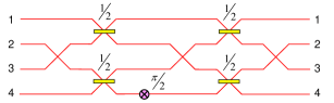
Figure 1: (Color online) The optical multiport circuit for 2-qubit QFT $F_{4}$.

Let $d=2^{m}$ be the number of modes for the $m$-qubit QFT multiport circuit. Using $F_{4}$ we can construct the $3$-qubit QFT $F_{8}$ as follows:

$$F_{8} (1,2,\ldots,8)=[S(2,3)\>S(4,5)\>S(6,7)]\>[S(3,4)\>S(5,6)]$$

$$\qquad[S(4,5)]\>[F_{4}(1,2,3,4)\>F_{4}(5,6,7,8)]$$

$$\qquad\left[P_{\frac{\pi}{4}}(6)\>P_{\frac{\pi}{2}}(7)\>P_{\frac{3\pi}{4}}(8)\right]\>[S(4,5)]\>[S(3,4)\>S(5,6)]$$

$$\qquad[S(2,3)\>S(4,5)\>S(6,7)]$$

$$\qquad[B(1,2)\>B(3,4)\>B(5,6)\>B(7,8)]$$

$$\qquad[S(2,3)\>S(4,5)\>S(6,7)]\>[S(3,4)\>S(5,6)]$$

$$\qquad[S(4,5)]$$ (3)

Fig. 2 shows a diagram for how circuits for $F_{4}$ is used for performing the $3$-qubit QFT $F_{8}$.

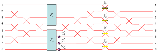
Figure 2: (Color online) Implementing 3-qubit QFT using a pair of multiport circuits for 2-qubit QFT.

To describe how to build $F_{2d}$ from $F_{d}$, it is convenient to define the shuffle operation $\Sigma$ that performs the following permutation on $2d$ modes:

$$(1,2, \ldots,2d)\mapsto$$

$$(1,d+1,2,d+2,\ldots,k,d+k,\ldots,d,2d).$$ (4)

Let $\Sigma^{-1}$ denote the inverse permutation.

Observe that $\Sigma(1,2,\dots,2d)$ can be realized with a PIC using $\frac{d(d-1)}{2}$ swap gates:

$$\Sigma (1,2,\ldots,2d)=[S(d,d+1)][S(d-1,d)\>S(d+1,d+2)]$$

$$\qquad[S(d-2,d-1)\>S(d,d+1)\>S(d+2,d+3)]\cdots$$

$$\qquad[S(2,3)S(4,5)\cdots S(n-2,n-1)].$$ (5)

Thus,

$$F_{2d} (1,2,\ldots,2d)=\left[\Sigma^{-1}(1,2,\ldots,2d)\right]$$

$$\qquad[F_{d}(1,2,\ldots,d)\>F_{d}(d+1,d+2,\ldots,2d)]$$

$$\qquad\left[P_{\frac{\pi}{d}}(d+2)\cdots P_{\frac{k\pi}{d}}(d+k+1)\cdots P_{\frac{(d-1)\pi}{d}}(2d)\right]$$

$$\qquad\left[\Sigma(1,2,\ldots,2d)\right]$$

$$\qquad[B(1,2)\>B(3,4)\cdots B(2d-1,2d)]$$

$$\qquad\left[\Sigma^{-1}(1,2,\ldots,2d)\right]$$ (6)

Let $N(F_{d})$ denote the number of optical elements needed for the $d$-dimensional QFT multiport circuit. With $N(F_{2})=1$ and $N(F_{4})=8$, we get the following recursive formula for the circuit size:

$$N(F_{2d})=2N(F_{d})+\frac{3d\left(d-1\right)}{2}+d+\left(d-1\right).$$ (7)

The first term in the sum on the right-hand-side corresponds to a pair of QFT circuits on $d$ modes, the second term counts the total number of swap gates, the third term counts the equal beam splitters, and the last term counts the phase shifters. Expressed as a function of $d$, we have

$$N(F_{d})=\frac{3d^{2}+d\left(\log_{2}{d}-7\right)}{4}+1$$ (8)

so the total number of elements in the multiport circuit is quadratic in the number of modes, as expected.

The recursive scheme works not just for qubits but for any QFT circuit with an even number of modes. More precisely, given an initial QFT circuit $F_{n}$, the scheme can be used to implement QFT for $d=n2^{k}$, where $k$ is a positive integer.

The scheme is essentially equivalent to a PIC translation of an important matrix factorization of Fourier matrices, initially discovered by Gauss Strang (1993) and a precursor to algorithms that perform fast Fourier transform Cooley and Tukey (1965):

$$F_{2d}=\frac{1}{\sqrt{2}}\begin{pmatrix}I_{d}&D_{d}\\ I_{d}&-D_{d}\end{pmatrix}\begin{pmatrix}F_{d}&0\\ 0&F_{d}\end{pmatrix}P$$ (9)

where $F_{d}$ is the $d$-dimensional Fourier matrix, $I_{d}$ is the $d$-dimensional identity matrix, $D_{d}=\mathrm{diag}\left(1,\omega,\ldots,\omega^{d}\right)$ is a diagonal matrix with $\omega=e^{2\pi i/d}$, and $P$ is the $2d\times 2d$ permutation matrix that maps the column vector $\vec{v}=\left(v_{1},v_{2},\ldots,v_{2d}\right)^{T}$ into

$$P\vec{v}=\left(v_{1},v_{3},\ldots,v_{2d-1},v_{2},v_{4},\ldots,v_{2d}\right)^{T},$$ (10)

that is, it shuffles components of $\vec{v}$ such that the first half involves components with odd indices and the second part involves the even ones. Note that $P$ is actually the matrix representing the permutation $\Sigma^{-1}$.

It is important to note that linear optical implementations of QFT have been previously explored by Törmä, et al. P. Törmä and Stenholm (1996), and Barak and Ben-Aryeh Barak and Ben-Aryeh (2007). Törmä, et al. examine the sufficient number of beam splitters needed for totally symmetric mode couplers, of which the discrete Fourier transform is a special case. Their calculations show that for a $d$-mode circuit, $(d\log_{2}d)/2$ beam splitters are sufficient. On the other hand, Barak and Ben-Aryeh describe a particular linear optical scheme for QFT based on the Cooley-Tukey algorithm.

A crucial difference between our scheme and these other approaches is that we are restricted to beam splitters that operate only on adjacent modes, since this is a limitation on PICs. This is why our scheme generally requires more beam splitters, in order to perform those additional swap operations. Both of the previous schemes were designed with bulk optics in mind, so they do not consider this restriction.

For QFT, all three approaches are formally equivalent through Eq. 9. In fact, the same number of equal beam splitters is used in all schemes; it is the number of phase shifters that vary.

Törmä, et al. provide a general formula for the matrix factorization they used but it does not completely specify where phase shifts are actually needed, since they are mostly concerned with counting the beam splitters.

Barak and Ben-Aryeh describe a specific Cooley-Tukey factorization of $d$-dimensional Fourier matrices into $\log_{2}d$ unitary operations that contain $d/2$ pairs of beam splitters and phase shifters, i.e., the phase shifts are always coupled to a beam splitter. We note that a recent experiment by Crespi, et al. Crespi et al. (2015) for testing the quantum suppression law Tichy et al. (2014) implements the Barak and Ben-Aryeh circuits for four- and eight-mode QFT on a 3-D PIC.

In contrast, our scheme employs $d-3$ phase shifters for $d$-mode QFT, so we achieve a modest savings on phase shifters. For example, the $3$-qubit QFT circuit of Barak and Ben-Aryeh uses 12 phase shifters but ours uses only 5. It may be worth mentioning that if one actually implements our QFT circuit with bulk optics, or a 3-D PIC such as in Ref. Crespi et al. (2015), where the swap gates do not involve beam splitters, our circuit is slightly more efficient because it requires fewer phase shifters.

III The inversion step in Grover’s algorithm

Grover’s algorithm Grover (1996) describes a quantum algorithm for searching an unsorted database of $d$ items using $O(\sqrt{d})$ calls to an oracle, which offers a quadratic speedup over known classical methods. In the most basic scenario, we have a database with $d$ items and we are supplied with a quantum oracle that can mark the solution to the search problem by shifting the phase of the solution’s register. The goal of the algorithm is to find the solution using the smallest number of queries.

To start, we prepare the equal superposition state

$$\left|\psi\right\rangle=\frac{1}{\sqrt{d}}\sum_{x=1}^{d}\left|x\right\rangle,$$ (11)

where $d=2^{m}$ is the number of basis states $\left|x\right\rangle$ for $m$ qubits.

Grover’s algorithm is then characterized by the repeated use of a quantum subroutine known as the Grover operator

$$G=\left(2|\psi\rangle\langle\psi|-I\right)O,$$ (12)

where $O$ is a query to the oracle and

$$W=2|\psi\rangle\langle\psi|-I$$ (13)

is often called the inversion about the mean. We shall refer to $W$ as Grover inversion. In this section, we describe a recursive multiport scheme for implementing Grover inversion on a PIC. In particular, the multiport circuit for searching $d$ items is utilized as a building block to the circuit for searching $2d$ items.

If we consider a search problem with a unique solution, the oracle can be realized by a single $\pi$-phase shift on the optical mode corresponding to the item to be marked.

To describe the main result, it is helpful to first consider the unitary transformation $V_{d}$, which involves a relatively simple network of equal beam splitters on $d$ modes. Using the multiport notation presented in Section II, we have

$$V_{4}(1,2,3,4) =[B(1,2)\>B(3,4)]\>[S(2,3)]$$

$$\qquad[B(1,2)\>B(3,4)]\>[S(2,3)].$$ (14)

The multiport circuit for $V_{4}$ is depicted in Fig. 3.

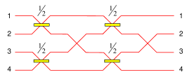
Figure 3: (Color online) The optical multiport circuit for the unitary $V_{4}$.

From $V_{4}$, we can build any other circuit $V_{d}$ for $d=2^{k}$ modes according to the rule

$$V_{2d} (1,2,\ldots,2d)=[V_{d}(1,\ldots,d)\>V_{d}(d+1,\ldots,2d)]$$

$$\qquad[\Sigma(1,2,\ldots,2d)][B(1,2)\>B(3,4)\cdots B(2d-1,2d)]$$

$$\qquad\left[\Sigma^{-1}(1,2,\ldots,2d)\right],$$ (15)

where $\Sigma$ is the same shuffle operator defined in Eq. (5). As an example, the circuit for $V_{8}$ is shown in Fig. 4 .

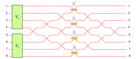
Figure 4: (Color online) Implementing the unitary $V_{8}$ using two multiport circuits for $V_{4}$.

Let $W_{d}$ denote Grover inversion on $d$ modes. First let us consider $W_{4}$, which is given by

$$W_{4} (1,2,3,4)=[S(1,2)\>S(3,4)]\>[B(1,2)\>B(3,4)]\>[S(2,3)]$$

$$\qquad[S(1,2)]\>[S(2,3)]\>[B(1,2)\>B(3,4)].$$ (16)

Fig. 5 shows how $W_{4}$ can be implemented with integrated optics.

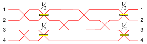
Figure 5: (Color online) The optical multiport circuit for Grover inversion $W_{4}$.

In the general case, it is convenient to define the unitary operation $\Phi$ on $2d$ modes that exchanges the photon amplitude in mode $1$ and mode $d+1$ through the following network of swap gates on neighboring modes:

$$\Phi (1,2,\ldots,2d)=[S(d,d+1)]$$

$$\>[S(1,2)\>S(3,4)\cdots S(d-1,d)]$$

$$\>[S(2,3)\>S(4,5)\cdots S(d-2,d-1)]\cdots$$

$$\>\left[S\left(\frac{d}{2},\frac{d}{2}+1\right)\right]\left[S\left(\frac{d}{2}-1,\frac{d}{2}\right)\>S\left(\frac{d}{2}+1,\frac{d}{2}+2\right)\right]$$

$$\>\cdots[S(1,2)\>S(3,4)\cdots S(d-1,d)][S(d,d+1)].$$ (17)

It is worth mentioning that $\Phi(1,2\ldots,2d)$ employs a total of $\frac{d^{2}}{4}+\frac{d}{2}+1$ swap gates.

The general multiport circuit for Grover inversion $W_{2d}$ employs both $W_{d}$ and $V_{d}$, and is given by

$$W_{2d} (1,2,\ldots,2d)=\left[W_{d}(1,\ldots d)\>W_{d}(d+1,\ldots,2d)\right]$$

$$\>[V_{d}(1,\ldots d)\>V_{d}(d+1,\ldots,2d)][\Phi(1,2,\ldots,2d)]$$

$$\>[V_{d}(1,\ldots d)\>V_{d}(d+1,\ldots,2d)].$$ (18)

Fig. 6 illustrates how the rule is used for building the circuit for $W_{8}$.

Figure 6: (Color online) Implementing Grover inversion $W_{8}$ using pairs of multiport circuits for $W_{4}$ and $V_{4}$.

Counting the number of optical elements used in $W_{2d}$, first for the unitary $V_{d}$, we have

$$N\left(V_{2d}\right)=2N(V_{d})+d(d-1)+d,$$ (19)

where the first term refers to a pair of $V_{d}$ circuits, the second term refers to the elements in $\Sigma$ and $\Sigma^{-1}$, and the last term refers to a set of parallel equal beam splitters on neighboring modes. Solving the formula with $N\left(V_{4}\right)=6$, we obtain

$$N\left(V_{d}\right)=\frac{d(d-1)}{2}.$$ (20)

Now for Grover inversion, we have

$$N\left(W_{2d}\right)=2N\left(W_{d}\right)+4N\left(V_{d}\right)+d^{2}+d+1,$$ (21)

where $N(W_{4})=9$. Plugging in $N\left(V_{d}\right)$ and solving the relation yields

$$N\left(W_{d}\right)=\frac{9d^{2}-d\left(6\log_{2}{d}+4\right)}{8}-1.$$ (22)

The recursive scheme directly implies that the $W_{d}$ has a matrix decomposition given by

$$W_{2d} =\begin{pmatrix}V_{d}&0\\ 0&V_{d}\end{pmatrix}Q\begin{pmatrix}V_{d}&0\\ 0&V_{d}\end{pmatrix}\begin{pmatrix}W_{d}&0\\ 0&W_{d}\end{pmatrix},$$ (23)

$$V_{2d} =\left(H\otimes I_{d}\right)\begin{pmatrix}V_{d}&0\\ 0&V_{d}\end{pmatrix},$$ (24)

where $I_{d}$ is the $d$-dimensional identity matrix,

$$W_{2} =\begin{pmatrix}0&1\\ 1&0\end{pmatrix}, V_{2} =H=\frac{1}{\sqrt{2}}\begin{pmatrix}1&1\\ 1&-1\end{pmatrix},$$ (25)

and $Q$ is the $2d\times 2d$ permutation matrix that exchanges the first and $(d+1)$th entry of a column vector. Unlike in the QFT circuit, the construction for Grover inversion is known only to work when $d=2^{k}$, because we do not know of any natural counterpart to $V_{d}$ when $d$ is not a power of two.

IV Multiport circuit simulations

In realistic linear optical systems, optical elements experience photon losses, optical modes suffer from relative phase mismatches, and fabrication defects lead to errors in the splitting ratios of beam splitters. To account for such device imperfections, we follow the example of Ref. Mower et al. (2015) and consider a simple model for silicon-based PICs that use directional couplers Mikkelsen et al. (2014) for beam splitters and thermo-optic phase modulators Harris et al. (2014) for phase shifters.

In this section, we simulate experiments on our multiport circuits and assess their performance under a fabrication model that focuses on two primary sources of errors: (i) incorrect reflectivities in beam splitters and (ii) absorption losses in the phase shifters.

For directional couplers, the error in the splitting ratio is due to imperfections in the dimensions of the coupled waveguides. In our model, we assign reflectivities to the beam splitters in the multiport circuits according to a Gaussian distribution, with mean 0.5 and standard deviation 0.04, which agrees with the testing data on recently developed devices Mikkelsen et al. (2014).

For thermo-optic modulators, the important source of error is the free-carrier absorption in doped silicon material, leading to propagation loss. Typically, the absorption process is modeled as a unitary operation by introducing a beam splitter between the lossy mode and an ancillary one, and whose transmissivity represents the photon loss rate for the device. Fortunately, the matrix representing a phase shifter is always block diagonal in the circuit. It is therefore sufficient to apply a scaling factor $\sqrt{1-\gamma}$ on the lossy mode, where $\gamma$ is the absorptivity. In our model, we assign $\gamma$ values to the phase shifters according to a rectified Gaussian distribution, with mean $0.05$ and standard deviation $0.025$, consistent with the reported loss rates in the latest studies Harris et al. (2014).

Our scheme also utilizes a significant number of swap gates, each of which can be realized by a beam splitter with vanishing reflectivity. However, it may be possible to implement the swap more efficiently since there is no required interaction between the modes. As such, we chose to model them as slightly better performing beam splitters, whose reflectivities are drawn from a rectified Gaussian distribution of mean 0.02 and standard deviation 0.02.

The first experiment we considered involves implementing the QFT circuit with randomly generated inputs of the form

$$\left|\phi_{4}\right\rangle =\left(z_{1},z_{2},z_{3},z_{4}\right)^{T}/\zeta_{4}$$

in the $2$-qubit case and

$$\left|\phi_{8}\right\rangle =\left(z_{1},z_{2},z_{3},z_{4},z_{5},z_{6},z_{7},z_{8}\right)^{T}/\zeta_{8}$$

in the $3$-qubit case where $z_{i}=\sqrt{-2\ln x_{i}}\exp\left(2\pi y_{i}\right)$ and $\zeta_{j}=\sum_{i=1}^{j}|z_{i}|^{2}$. The parameters $x_{i}$ and $y_{i}$ were all picked independently and uniformly at random from the interval $(0,1)$.

It is known that a Haar-random $d$-dimensional pure state may be constructed by normalizing a vector of $d$ independent, identically distributed complex Gaussian random variables Żykowski and Sommers (2001). Thus, the above procedure for generating input states is equivalent to sampling random pure quantum states from the uniform Haar measure, since $z_{i}$ represents the Box-Muller transform Box and Muller (1958), which generates a pair of Gaussian random numbers from a pair of uniformly distributed ones.

To evaluate the performance of our circuits, we calculated the (squared) fidelity $F(\Psi,\Phi)=|\left\langle\Psi|\Phi\right\rangle|^{2}$ between the simulated output state $\left|\Phi\right\rangle$ and the ideal output $\left|\Psi\right\rangle$ for each particular input. Because of the Haar-random sampling of input states, the mean fidelity we get provides a good estimate of the average gate fidelity for the QFT circuit, a fairly common figure of merit for quantum gate experiments.

After running $10^{7}$ trials, we obtained fidelities with a mean value of $0.94$ and a standard deviation of $0.032$ in the 2-qubit case, and a mean value of $0.86$ and a standard deviation of $0.056$ in the 3-qubit case.

The second experiment involves running Grover’s algorithm on four-item and eight-item databases, each with a unique solution. In contrast with the first experiment, Grover’s algorithm specifically uses the equal superposition state as its input. Thus, we have included the gates required for preparing this state in our simulation.

The multiport circuit for a four-item Grover search is illustrated in Fig. 7. The schematic for the eight-item version is displayed in Fig. 8, where the dashed boxes refer to oracle queries realized by a $\pi$-phase shift on the appropriate mode, and the circuit $P_{8}$ for preparing the input is shown separately in Fig. 9.

Observe that the oracle query and Grover inversion are repeated twice in the $8$-item quantum search, which follows from the fact that Grover’s algorithm prescribes doing $\left\lfloor\frac{\pi}{4}\sqrt{d}\right\rfloor$ iterations, which is 2 when $d=8$. In this case, Grover’s algorithm produces an output state that generates the solution with high probability $\left(\frac{121}{128}\approx 0.945\right)$, not deterministically.

We performed $10^{7}$ trials for both searches, each with a randomly selected unique solution. For each trial we computed the fidelity of the simulated output with the ideal one. We obtained fidelities with a mean of $0.90$ and a standard deviation of $0.051$ for a four-item Grover search, and a mean of $0.76$ and a standard deviation of $0.099$ for an eight-item Grover search

We must emphasize that what these results indicate is the feasibility of a classical simulation of Grover’s algorithm with our circuits. Nevertheless, like QFT, it is possible that the unitary $W_{d}$ may find suitable application in some other truly quantum setting.

There have been no linear optical experiments to date to which we can directly compare our simulation values; however, recent demonstrations on PIC devices have obtained fidelities of more than 0.94 Politi et al. (2008); Carolan et al. (2015). Considering that our simulations were done with a rudimentary yet conservative error model, it is encouraging to see a comparable level of performance with our multiport circuits.

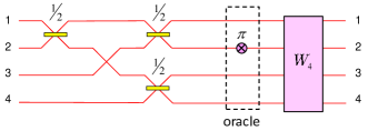
Figure 7: (Color online) The optical multiport circuit for Grover search on four items. In the diagram, the second mode represents the solution to the search problem. The output of the algorithm is obtained by a final measurement in the standard basis.

Figure 8: (Color online) The optical multiport circuit for Grover search on eight items. The box $P_{8}$ corresponds to the circuit in Fig. 9. In this diagram, the third mode represents the solution to the search problem. The output is obtained by a final measurement in the standard basis.

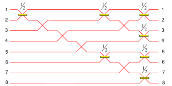
Figure 9: (Color online) The optical multiport circuit $P_{8}$ for preparing an equal superposition state for eight modes given an input photon in the first mode.

Experiment	Mean fidelity	Std. deviation
2-qubit QFT [8]	0.944	0.0319
4-item Grover [14]	0.904	0.0507
3-qubit QFT [41]	0.861	0.0559
8-item Grover [112]	0.762	0.0990

Table 1: Simulation fidelities for $10^{7}$ trials. The total number of beam splitters and phase shifters in each circuit is indicated in the brackets.

V Discussion

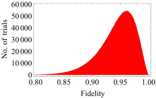
(a)

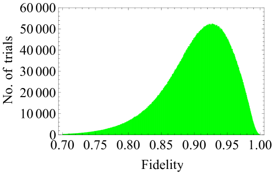
(b)

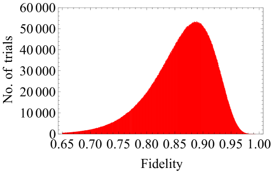
(c)

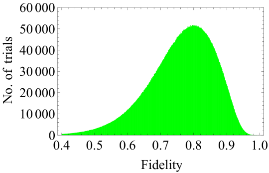
(d)

Figure 10: (Color online) Histograms of simulation results for (a) $2$-qubit QFT ($0.949$), (b) four-item Grover search ($0.912$), (c) $3$-qubit QFT ($0.870$), and (d) eight-item Grover search ($0.774$), with bin sizes obtained using the Freedman-Diaconis rule . The median values are indicated in parentheses.

Any $d$-dimensional unitary operation can be implemented with linear optics, by a triangular array of beam splitters on $d$ modes, each accompanied by a phase shifter, and another $d-1$ phase shifters Reck et al. (1994). Such a matrix decomposition requires $d^{2}-1$ optical elements, exactly the number of real parameters needed to specify a unitary in $\mathrm{SU}(d)$. While this specific arrangement might be preferred when trying to develop a fully reconfigurable linear optical processor, it is generally not the optimal choice for specific unitary families. If we wish to develop a quantum processor dedicated to a particular task, it may be possible, and quite desirable, to design a multiport circuit that uses fewer elements, since fabrication defects in devices are known to severely hamper the quantum performance of PICs. Furthermore, depending on how technological capabilities improve, photonic circuits that consist just of equal beam splitters and a small number of simple phase shifts might be more appropriate in certain contexts.

The recursive scheme described in this paper illustrates that for unitary operations that serve as major components of Shor’s and Grover’s algorithm, we can assemble a multiport circuit from smaller versions of the same operation. The matrix decompositions for QFT and Grover inversion both have a relatively simple structure, which is made seemingly complicated only because of permutations have to be implemented by a sequence of nearest-neighbor swap gates.

We have previously discussed the optical circuit size for QFT and Grover inversion. For completeness, we can also remark on the optical circuit depth in comparison to the unitary matrix factorization of Reck, et al. Let $D(U)$ denote the circuit depth for implementing $U$. In their case, the configuration of beam splitters and phase shifter is fixed for any arbitrary $d$-dimensional unitary so the circuit depth is $2(d-1)$ . For the QFT circuits, we have

$$D(F_{d})=3(d-1)-2\log_{2}d$$ (26)

while for the Grover inversion circuits, we have

$$D(W_{d})=5d-2\log_{2}d-(\log_{2}d)^{2}-6.$$ (27)

Thus, there is a linear dependence on $d$ in all cases, although our circuit depths are around a factor of 2 worse. This is precisely due to the swap operations in our scheme, which is quite unavoidable because elementary gates on a PIC are restricted to adjacent optical modes.

The simulation results listed in Table 1 show that these circuits perform well even when realistic errors in the optical elements are taken into account. This is accomplished even before we apply post-fabrication optimization techniques Mower et al. (2015) that would significantly improve the overall performance.

For a quick summary of the data, we include histograms of the fidelities in Fig. 10, where the bin size is determined by the Freedman-Diaconis rule. This gives a rough picture of how the fidelity values are distributed, in particular, how much are the values skewed to the left.

Nonetheless, it seems clear that further advances in fabrication methods will be needed to scale to much larger circuits. From the results of both experiments, we can roughly estimate a 9% to 15% reduction in average fidelity when the number of modes is doubled. This seems to be the case even though the number of elements in QFT increases fivefold while that of Grover’s algorithm increases eightfold. Still, this rate of decline implies the fidelity will go below acceptable levels rather quickly. It is previously known that errors of as high as 1% per elementary gate will still allow fault-tolerant quantum computing Knill (2005) but in terms of the overhead resources needed to protect against failures, we will likely require less than 0.1 % error per gate for a practical device.

There are other long-standing issues with integrated photonic platforms. One is the problem of integrating single photon sources and detectors with a silicon-based PIC. Some recent progress in this area include waveguide-integrated semiconductor quantum dot sources Murray et al. (2015) and superconducting nanowire detectors Najafi et al. (2015).

Another problem is that one typically needs to build customized chips for each experiment. Furthermore, settings may need to be reconfigured between different runs of the same experiment; for example, in an adaptive experiment, several device settings might be updated according to the outcome of intermediate measurements. These latter concerns will be addressed by a reprogrammable photonic quantum processor Mower et al. (2015); Carolan et al. (2015).

VI Concluding Remarks

Photonic approaches to quantum information processing has seen extensive growth over the last few years and linear optics has played a major role in many of the recent advances. In particular, optical implementations on integrated systems have vastly improved our ability to perform quantum experiments with single photons.

In this paper we described recursive multiport circuits for quantum Fourier transforms and Grover inversion. The circuits are designed to be implemented on linear optical networks where qudits are encoded in the path traversed by single photons. Each circuit requires $O(d^{2})$ optical devices for implementing a $d$-dimensional unitary operation, which shows that they scale in a reasonable manner. We also demonstrated that these circuits can achieve high-fidelity performance in a practical setting by conducting simulations on a silicon-based PIC model that incorporates the faulty operation of real optical devices.

Our recursive schemes take advantage of the natural modularity of photonic integrated circuits, allowing us to construct more sophisticated multiport circuits using smaller versions of the same operation as building blocks. This may prove beneficial for practical implementations because it provides a straightforward approach to scaling operations into higher dimensions. In contrast, if one for example uses the triangular array of Reck, et al.Reck et al. (1994), the phases and reflectivities in the circuit will generally require adjusting whenever more optical modes are added.

Our results show the versatility of PICs as a platform for developing high-quality, scalable quantum information processors. It is our hope that this work will help promote new avenues of research into integrated photonic devices and stimulate technological improvements that will allow more practical applications.