Proton-lambda correlation functions at the LHC
with account for residual correlations

Abstract

The theoretical analysis of $\bar{p}-\Lambda\oplus p-\bar{\Lambda}$ correlation function in 10% most central Au+Au collisions at RHIC energy $\sqrt{s_{NN}}=200$ GeV shows that the contribution of residual correlations is the necessary factor to obtain a satisfactory description of the experimental data. A neglecting of the residual correlation effect, leads to unrealistically low source radius, about 2 times smaller than the corresponding value for $p-\Lambda\oplus\bar{p}-\bar{\Lambda}$ case, when one fits the experimental correlation function within Lednický-Lyuboshitz analytical model. Recently an approach accounting effectively for residual correlations for the baryon-antibaryon correlation function was proposed, and a good RHIC data description was reached with the source radius extracted from the hydrokinetic model (HKM). The $\bar{p}-\Lambda$ scattering length, as well as the parameters characterizing the residual correlation effect — annihilation dip amplitude and its inverse width — were extracted from the corresponding fit. In this paper we use these extracted values and simulated in HKM source functions for Pb+Pb collisions at the LHC energy $\sqrt{s_{NN}}=2.76$ TeV to predict the corresponding $p\Lambda$ and $p\bar{\Lambda}$ correlation functions.

Keywords: final state interaction, baryons, lead-lead collisions, LHC, residual correlations

I Introduction

The study of $p\Lambda$ correlation functions (CF) (along with the study of other two-particle correlations such as $\pi\pi$, $KK$) allows one to obtain the information about the character of evolution of the matter formed in relativistic nuclear collisions, in particular about the character of collective flow.

Another great possibility which is open for a researcher in baryon-(anti)baryon correlation analysis is the study of strong interaction between the particles of different sorts with Final State Interaction (FSI) correlation technique Led ; fsi ; FsiSin . Since LHC produces copiously hadrons of different species, including multi-strange, charmed and beauty ones, the advantage of this approach is the ability to analyze the interactions even in exotic particle pairs, hardly achieved by other means.

Fitting the experimental correlation function with some analytical formula, e. g. Lednický-Lyuboshitz model Led , allows one to extract the quantities describing both the interaction in corresponding pairs and the particle emission region size. Of course, if the source function $S({\bf r}^{*})$, describing the spatial structure of the pair emission, is known, an extraction of unknown interaction parameters becomes more reliable. The corresponding spatial structure can be obtained from realistic collision model that simulates the evolution of the system formed in high energy heavy ion collisions. In the recent paper pLamOur the hybrid variant of the hydrokinetic model (HKM) HKM ; Boltz ; Kaon was used for this purpose. The choice of HKM is highly reliable since it is known to provide a successful simultaneous description of a wide class of bulk observables in nuclear collision experiments at RHIC and LHC Uniform . The model also reproduces well Sf the source functions for pion and kaon pairs in Au+Au collisions at the top RHIC energy Phenix , including non-Gaussian tails observed in certain experimental source function projections.

In pLamOur in order to extract unknown $\bar{p}\Lambda$ scattering length, the corresponding experimental correlation function for 10% most central Au+Au collisions at top RHIC energy, measured by STAR Collaboration Star , was fitted with the Lednický-Lyuboshitz formula using the effective source radius $r_{0}$ extracted from the HKM source function. It was also found that $r_{0}$ values obtained in HKM for baryon-baryon and baryon-antibaryon correlations are expectedly close, while in the STAR experimental analysis Star , where the source radii were considered as free fit parameters, the extracted $\bar{p}\Lambda$ radius was $\sim 2$ times smaller than the $p\Lambda$ one. One can assume that this apparent difference is due to neglect of residual correlations in Star . Such correlations can exist between secondary protons and lambdas if their parents were correlated (or the parent of one particle was correlated with another particle in the pair). For taking into account the residual correlation contribution to the baryon-antibaryon CF, a modified analytical formula was introduced in pLamOur . As a result, a good description of the experimental $\bar{p}\Lambda$ correlation function is obtained and the $\bar{p}\Lambda$ spin-averaged scattering length is extracted from the corresponding fit.

In the present paper we are going to apply the method developed in pLamOur for description of the RHIC data to predict the $p\Lambda$ and $\bar{p}\Lambda$ correlation functions in the 5% most central Pb+Pb collisions at the LHC energy $\sqrt{s_{NN}}=2.76$ TeV, utilizing the results of Ref. pLamOur as a starting point.

II Formalism

The experimental correlation functions presented in Star are purity corrected. They are obtained from the measured ones as

$$C_{\mathrm{corr}}(k^{*})=\frac{C_{\mathrm{meas}}(k^{*})-1}{\lambda(k^{*})}+1,$$ (1)

where $C_{\mathrm{meas}}(k^{*})$ and $C_{\mathrm{corr}}(k^{*})$ are the measured and the corrected CF respectively, and $\lambda(k^{*})$ is pair purity. The latter is defined as the fraction of pairs consisting of primary, correctly identified particles.

As well as in pLamOur we model the purity corrected LHC baryon-baryon correlation function with Lednický-Lyuboshitz analytical formula Led :

$$C(k^{*})=1+\sum_{S}\rho_{S}\left[\frac{1}{2}\left|\frac{f^{S}(k^{*})}{r_{0}}\right|^{2}\left(1-\frac{d_{0}^{S}}{2\sqrt{\pi}r_{0}}\right)\right.+$$

$$\left.\frac{2\mathop{\mathrm{Re}}\nolimits f^{S}(k^{*})}{\sqrt{\pi}r_{0}}F_{1}(2k^{*}r_{0})-\frac{\mathop{\mathrm{Im}}\nolimits f^{S}(k^{*})}{r_{0}}F_{2}(2k^{*}r_{0})\right],$$ (2)

where $F_{1}(z)=\int_{0}^{z}dxe^{x^{2}-z^{2}}/z$ and $F_{2}(z)=(1-e^{-z^{2}})/z$. This formula is derived starting from the basic equation $C(k^{*})=\left\langle\left|\Psi^{S}_{-\textbf{k}^{*}}(\textbf{r}^{*})\right|^{2}\right\rangle$, where the wave function $\Psi_{-\textbf{k}^{*}}^{S}$ represents the stationary solution of the scattering problem with the opposite sign of the vector $\textbf{k}^{*}$. The angle brackets mean averaging over the total spin $S$ and the distribution of the relative distances $S(\textbf{r}^{*})$. Since typically the source radius can be considered much larger than the range of the strong interaction potential, $\Psi_{-\textbf{k}^{*}}^{S}$ can be approximated at small $k^{*}$ by the s-wave solution in the outer region:

$$\Psi_{-\textbf{k}^{*}}^{S}(\textbf{r}^{*})=e^{-i\textbf{k}^{*}\cdot\textbf{r}^{*}}+\frac{f^{S}(k^{*})}{r^{*}}e^{ik^{*}\cdot r^{*}}.$$ (3)

The scattering amplitude $f^{S}(k^{*})$ here is taken in the effective range approximation

$$f^{S}(k^{*})=\left(\frac{1}{f^{S}_{0}}+\frac{1}{2}d^{S}_{0}k^{*2}-ik^{*}\right)^{-1},$$ (4)

where $f^{S}_{0}$ is the scattering length and $d^{S}_{0}$ is the effective radius for a given total spin $S=1$ or $S=0$. The singlet and triplet weights $\rho_{i}$ for unpolarized particles (supposing the polarization $P=0$) are in $\rho_{0}=1/4(1-P^{2})=1/4$ and $\rho_{1}=1/4(3+P^{2})=3/4$ correspondingly.

As for the baryon-antibaryon case, following pLamOur , we fit the experimentally measured correlation function $C_{uncorr}(k^{*})$ with the following analytical expression

$$C_{\mathrm{uncorr}}(k^{*})=1+\lambda(k^{*})(C(k^{*})-1)+\alpha(k^{*})(C_{\mathrm{res}}(k^{*})-1),$$ (5)

where $\lambda(k^{*})$ is purity or the fraction of correctly identified pairs consisting of primary particles, $C(k^{*})$ is “true” correlation function approximated by Eq. (II), $\alpha(k^{*})$ is the fraction of secondary particles which are residually correlated, $\alpha(k^{*})=\tilde{\alpha}(1-\lambda(k^{*}))$ and $C_{\mathrm{res}}(k^{*})$ is the residual correlation contribution. The latter is taken in the Gaussian form pLamOur ; StarPRL

$$C_{\mathrm{res}}(k^{*})=1-\tilde{\beta}e^{-4k^{*2}R^{2}},$$ (6)

where $\tilde{\beta}=A>0$ is the annihilation (wide) dip amplitude and $R\ll r_{0}$ is the dip inverse width. Since $\tilde{\alpha}$ and $\tilde{\beta}$ enter (5) only as a product $\tilde{\alpha}\tilde{\beta}$, the latter is treated as a single parameter $\beta$ at fitting.

The source radii $r_{0}$ in both $p\Lambda$ and $\bar{p}\Lambda$ cases are extracted from the Gaussian fit $S_{\mathrm{fit}}(r^{*})=(2\sqrt{\pi}r_{0})^{-3}e^{-\frac{r^{*2}}{4r_{0}^{2}}}$ to the angle averaged source function,

$$S(r^{*})=1/(4\pi)\int_{0}^{2\pi}\int_{0}^{\pi}S(r^{*},\theta,\phi)\sin\theta d\theta d\phi,$$ (7)

calculated in the hydrokinetic model HKM ; Boltz ; Kaon . The latter simulates the evolution of the matter in relativistic nuclear collision as consisting of two stages — the hydrodynamic expansion of the matter being in local thermal and chemical equilibrium and gradual system decoupling, beginning when the equilibrium is lost. The first stage is described within ideal hydrodynamics and for the second one the hydrokinetic approach is utilized, based on the Boltzmann equations in the integral form, with switching to UrQMD cascade at a space-like hypersurface. In current study HKM is taken in its simplified hybrid form Uniform with sudden switch from hydrodynamic evolution to the cascade at the hadronization hypersurface defined by the isotherm $T=165$ MeV.

The model output consists of generated particle momenta and coordinates, that are further used to build different observables. The considered angle-averaged source function histograms are filled using the following procedure (here $r^{*}$ is the particle spatial separation in the pair rest frame)

$$S({r}^{*(k)})=\frac{\sum_{n=1}^{N_{\mathrm{ev}}}\sum_{i_{1}^{n},i_{2}^{n}}[\delta_{\Delta}(r^{*(k)}-r^{*}_{i_{1}^{n}}+r^{*}_{i_{2}^{n}})/(4\pi(r^{*}_{i_{1}^{n}}-r^{*}_{i_{2}^{n}})^{2}\Delta)]}{\sum_{n=1}^{N_{\mathrm{ev}}}\sum_{i_{1}^{n},i_{2}^{n}}1}$$ (8)

Here ${r}_{i_{1}^{n}}^{*}$ and ${r}_{i_{2}^{n}}^{*}$ are the pair rest frame $r$-coordinates of particles 1 and 2 produced in the $n-$th event, ${r}^{*(k)}$ is the $r$-coordinate of the $k$-th histogram bin center, the function $\delta_{\Delta}(x)=1$ if $|x|<\Delta/2$ and $0$ otherwise, and $\Delta$ is the size of the histogram bin.

III Results and discussion

The initial conditions (IC) for HKM calculations simulating the considered case of 5% most central Pb+Pb collisions at the LHC energy $\sqrt{s_{NN}}=2.76$ TeV are described in detail in Uniform ; Shap . We assume longitudinal boost invariance, so that the IC are specified in the plane transverse to the beam axis only. The transverse energy density profile $\epsilon_{i}(\textbf{r}_{T})$ at the starting time $\tau_{i}=0.1$ fm/$c$ corresponds to Monte Carlo Glauber model and is calculated in GLISSANDO code Gliss , where the overall scale factor $\epsilon_{0}$, being the maximal initial energy density, is fixed basing on the experimental mean charged particle multiplicity. The initial transverse flow in present calculations is absent.

In Fig. 1 one can see the angle averaged $p\Lambda$ source function $S(r^{*})$ obtained in hydrokinetic model for considered LHC collisions together with the Gaussian fit to it. The source radius value extracted from this fit is $r_{0}=3.76$ fm, which is about 1.15 times larger than for the RHIC case. The $\bar{p}\Lambda$ source function fitting results in the same source radius value.

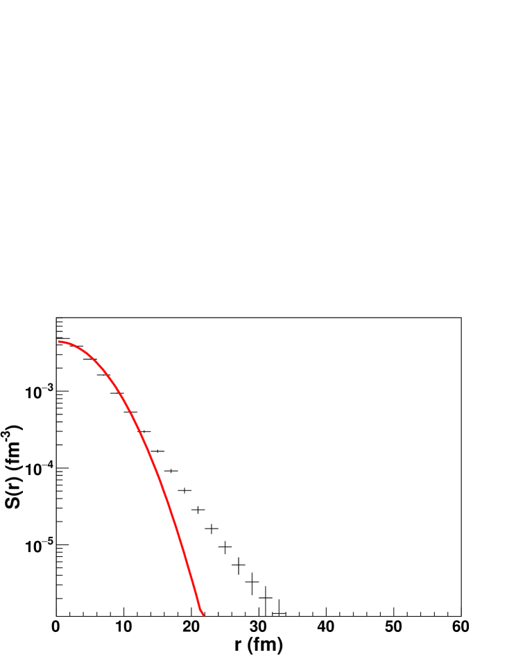
Figure 1: The $p\Lambda$ angle averaged source function calculated in HKM (markers) and the Gaussian fit to it (line). The calculations correspond to 5$\%$ most central Pb+Pb collisions at LHC energy $\sqrt{s_{NN}}=2.76$ TeV, in pseudorapidity range $|\eta|<0.8$. Proton $p_{T}$ range is $0.7<p_{T}<4$ GeV/$c$, and for lambdas $0.7<p_{T}<5$ GeV/$c$. The extracted $r_{0}=3.76$ fm.

Having obtained $r_{0}$ from HKM and fixing $f^{S}_{0}$ and $d^{S}_{0}$ according to the paper Wang for baryon-baryon case, we can model the corresponding correlation function (see Fig. 2). As compared to RHIC, the LHC $p\Lambda$ CF is slightly more narrow (the two corresponding Gaussian widths differ by a factor of $\sim 1.13$) and has lower intercept of about 1.7.

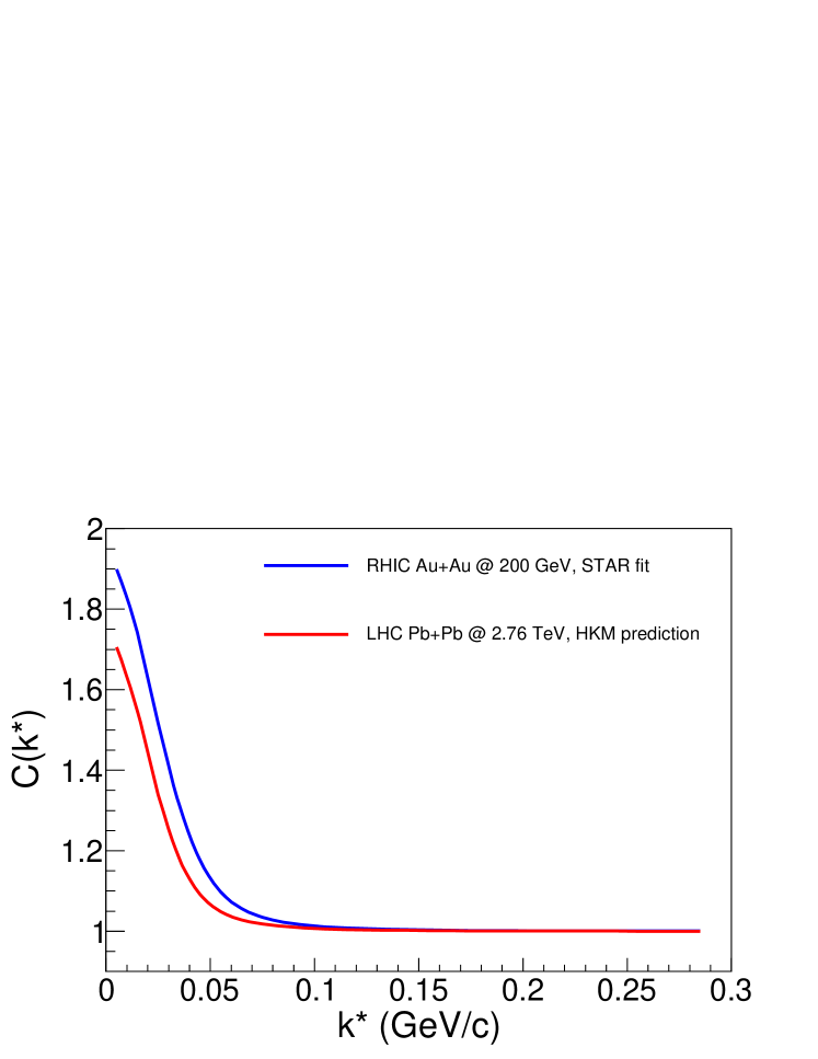
Figure 2: The HKM prediction for purity corrected $p-\Lambda\oplus\bar{p}-\bar{\Lambda}$ correlation function in the LHC Pb+Pb collisions at $\sqrt{s_{NN}}=2.76$ TeV, $c=0-5\%$, $|\eta|<0.8$, with $0.7<p_{T}<4$ GeV/$c$ for protons and $0.7<p_{T}<5$ GeV/$c$ for lambdas (red line). The LHC source radius value calculated in HKM is $r_{0}=3.76$ fm. The Lednický-Lyuboshitz fit to the top RHIC energy correlation function, corresponding to the STAR experiment Star , with $r_{0}=3.23$ fm extracted from the HKM source function is presented for comparison (blue line).

To build the corresponding baryon-antibaryon correlation function one should determine the values of parameters entering (5) and (6) for the LHC case. As well as for RHIC we assume $f^{s}=f^{t}=f$ and $d^{s}_{0}=d^{t}_{0}=0$. The source radius is again fixed from HKM calculation, $r_{0}=3.76$ fm. As for the real and imaginary parts of the scattering length, $\mathop{\mathrm{Re}}\nolimits f_{0}$ and $\mathop{\mathrm{Im}}\nolimits f_{0}$, they characterize antiproton-lambda strong interaction and hence are not changed when switching from RHIC to LHC. So we can use the values extracted from the fit to RHIC $\bar{p}\Lambda$ correlation function shown in Fig. 6 of the paper pLamOur , where the Gaussian parametrization (6) for the residual correlation contribution $C_{\mathrm{res}}(k^{*})$ is applied, $\mathop{\mathrm{Re}}\nolimits f_{0}=0.14\pm 0.66$ fm and $\mathop{\mathrm{Im}}\nolimits f_{0}=1.53\pm 1.31$ fm. The parameter $\beta=\tilde{\alpha}\tilde{\beta}$ describes the strength of residual correlations and the fraction of residually correlated non-primary particles. So, this parameter depends on particle interaction kinematics. Thus, it also can be taken the same as for RHIC, $\beta=0.034\pm 0.005$. As for the $R$ parameter, being some effective size associated with residual correlations ($R_{\mathrm{RHIC}}=0.48\pm 0.05$ fm), one can suppose that for LHC it will be larger than for RHIC, approximately proportionally to the source radii ratio $r_{0}^{\mathrm{LHC}}/r_{0}^{\mathrm{RHIC}}\approx 1.15$, i. e. $R_{\mathrm{LHC}}=R_{\mathrm{RHIC}}(r_{0}^{\mathrm{LHC}}/r_{0}^{\mathrm{RHIC}})$. Such an assumption gives $R_{\mathrm{LHC}}=0.55\pm 0.06$ fm . Note, that since the mentioned parameter values have errors, the LHC correlation function cannot be predicted exactly, but only up to uncertainties caused by these errors in the fit parameters. The uncertainty in the predicted correlation function is calculated as $\Delta C_{\mathrm{uncorr}}(k^{*})=\sqrt{\sum_{i=1}^{4}\left(\frac{\partial C_{\mathrm{uncorr}}(k^{*})}{\partial x_{i}}\right)^{2}\sigma_{i}^{2}+2\sum_{1\leq i<j\leq 4}\frac{\partial C_{\mathrm{uncorr}}(k^{*})}{\partial x_{i}}\frac{\partial C_{\mathrm{uncorr}}(k^{*})}{\partial x_{j}}\sigma_{ij}}$, where $x_{i}$ are the 4 fit parameters, $\mathop{\mathrm{Re}}\nolimits f_{0}$, $\mathop{\mathrm{Im}}\nolimits f_{0}$, $\beta$ and $R$, $\sigma_{i}=\Delta x_{i}$ are the corresponding parameter standard errors, and $\sigma_{ij}$ are the covariances of parameters $x_{i}$ and $x_{j}$.

The determination of purity $\lambda(k^{*})$ at the LHC is not so explicit, since it depends not only on the fraction of secondary pairs, coming from resonance decays, but also on the experimental setup, or more precisely, on the fraction of misidentified pairs. To clarify this issue we have calculated the fractions of pairs made by particles having different origination (primary or coming from certain decays) in the hydrokinetic model for RHIC and LHC collisions. The results obtained in both cases are quite close and are presented in Table I. Comparing these fractions with those in Table III for RHIC Star , one can see that experimental fraction of $p_{prim}-\Lambda_{prim}$ pairs $\lambda=0.15$ is about 2.5 times lower than in HKM, likely due to misidentification problem, which takes place in the experiment. In HKM simulations, on the contrary, all the produced particles are correctly identified, that leads to such a difference between corresponding fraction values. However, since HKM is a realistic model that describes both RHIC and LHC bulk observables well, basing on its results one can conclude, that true purities, understood as the fractions of primary pairs, at RHIC and LHC should be quite similar.

Pairs	Fractions (%)
$p_{prim}-\Lambda_{prim}$	$38$
$p_{\Lambda}-\Lambda_{prim}$	$16$
$p_{\Sigma^{+}}-\Lambda_{prim}$	$3$
$p_{prim}-\Lambda_{\Sigma^{0}}$	$12$
$p_{\Lambda}-\Lambda_{\Sigma^{0}}$	$5$
$p_{\Sigma^{+}}-\Lambda_{\Sigma^{0}}$	$1$
$p_{prim}-\Lambda_{\Xi}$	$17$
$p_{\Lambda}-\Lambda_{\Xi}$	$7$
$p_{\Sigma^{+}}-\Lambda_{\Xi}$	$1$

Table 1: The fractions of $p\Lambda$ pairs, primary and coming from different decays calculated in HKM. These fractions are quite similar for RHIC and LHC cases.

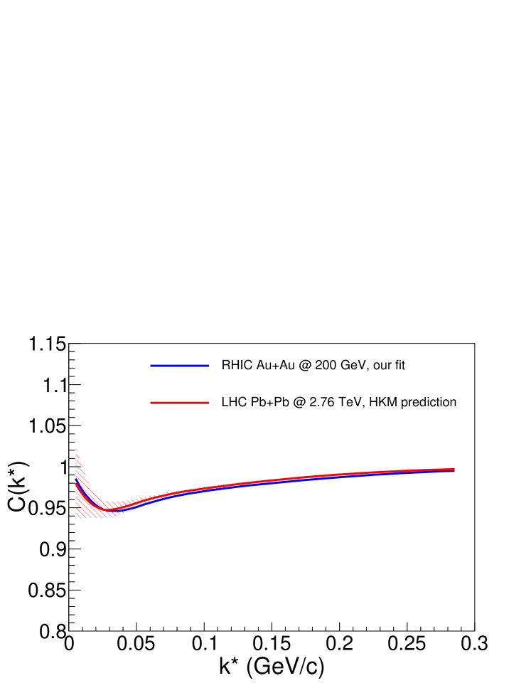
Figure 3: The same as in Fig. 2 for purity uncorrected $\bar{p}-\Lambda\oplus p-\bar{\Lambda}$ correlation function. The HKM source radius for LHC is $r_{0}=3.76$ fm. The purity $\lambda(k^{*})$ is the same as for RHIC case Star . The scattering length real and imaginary parts, $\mathop{\mathrm{Re}}\nolimits f_{0}$ and $\mathop{\mathrm{Im}}\nolimits f_{0}$, are taken from the fit to RHIC CF that corresponds to Fig. 6 from pLamOur , where HKM source radius $r_{0}=3.28$ fm and the Gaussian parametrization (6) for the residual correlation contribution $C_{\mathrm{res}}(k^{*})$ are utilized. For the LHC fit the $C_{\mathrm{res}}(k^{*})$ parameter $\beta$ coincides with that for RHIC, while parameter $R$ is scaled by the factor $r_{0}^{\mathrm{LHC}}/r_{0}^{\mathrm{RHIC}}$. The LHC fit is determined up to errors in parameters $\mathop{\mathrm{Re}}\nolimits f_{0}$, $\mathop{\mathrm{Im}}\nolimits f_{0}$, $\beta$ and $R$, that is illustrated by the band around the LHC curve.

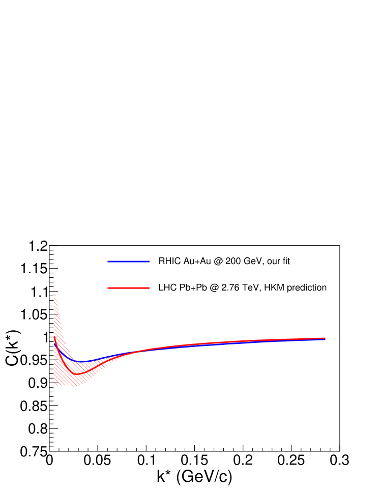
Figure 4: The same as in Fig. 3, but LHC purity $\lambda(k^{*})$ is scaled as compared to RHIC according to primary $p\Lambda$ pairs fraction in HKM simulations, where there is no misidentification problem.

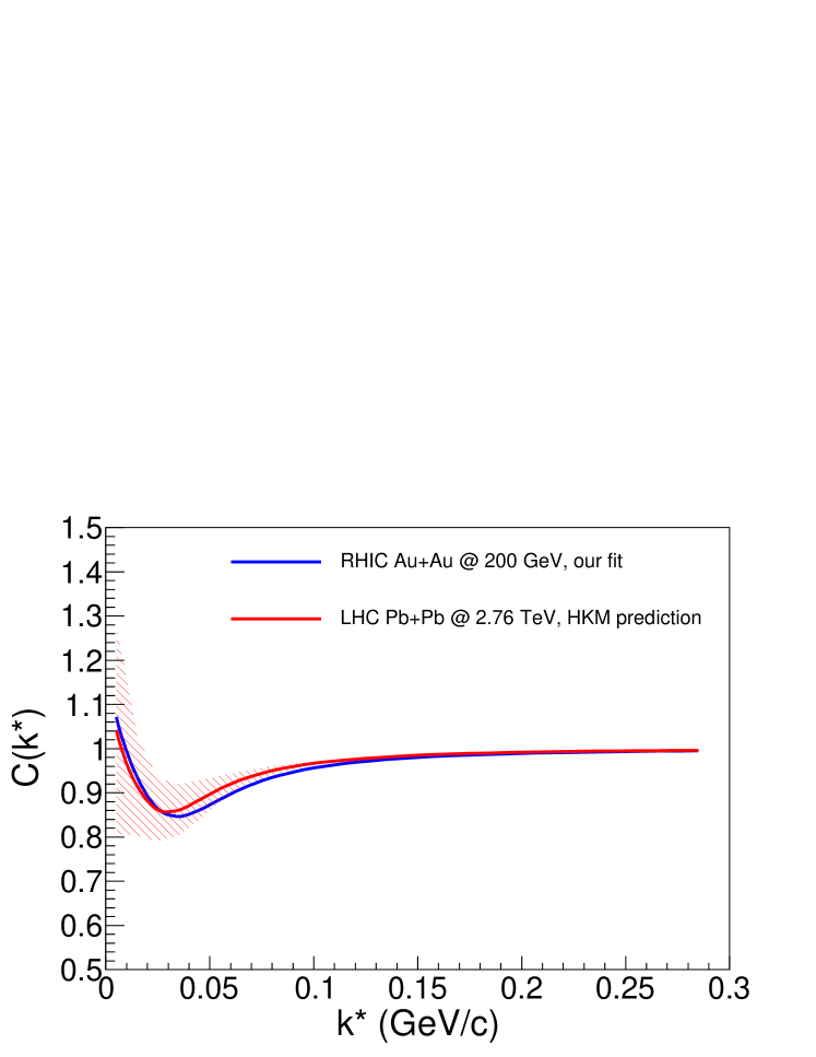
Figure 5: The same as in previous two figures, but the correlation functions are corrected for purity and residual correlations, i. e. $C(k^{*})=1+(C_{\mathrm{uncorr}}(k^{*})-1)/\lambda(k^{*})-\alpha(k^{*})(C_{\mathrm{res}}(k^{*})-1)/\lambda(k^{*})$.

In such a situation we demonstrate three different plots for the LHC $\bar{p}-\Lambda\oplus p-\bar{\Lambda}$ correlation function (see Fig. 3–5). The first one demonstrates the model CF with $\lambda_{\mathrm{LHC}}(k^{*})$ the same as for RHIC Star , $\lambda_{\mathrm{LHC}}(k^{*})=\lambda_{\mathrm{RHIC}}(k^{*})$. This function is again more narrow than for RHIC. In Fig. 4 one can see our prediction for the LHC correlation function with $\lambda_{\mathrm{LHC}}(k^{*})=2.5\lambda_{\mathrm{RHIC}}(k^{*})$, where the factor 2.5 corresponds to the ratio of corresponding primary pairs’ fractions in HKM and in the STAR experiment. As for Fig. 5, it shows the purity and residual correlation corrected CFs for LHC and RHIC. They are expressed (as it follows from Eq. (5)) through the uncorrected ones as $C(k^{*})=1+(C_{\mathrm{uncorr}}(k^{*})-1)/\lambda(k^{*})-\alpha(k^{*})(C_{\mathrm{res}}(k^{*})-1)/\lambda(k^{*})$. The latter “true” function can be easily compared with the experimental result (corrected in the same way for purity and residual correlations), since it does not depend on the fraction of misidentified particles in the concrete experiment. As compared to RHIC, the LHC curve apparently has smaller amplitude and width.

IV Conclusions

The first predictions for $p\Lambda$ and $\bar{p}\Lambda$ correlation functions, calculated within Lednický-Lyuboshitz and hydrokinetic (HKM) models and accounting for the residual correlation effect, are presented for the 5% most central Pb+Pb LHC collisions at the energy $\sqrt{s_{NN}}=2.76$ TeV. The functions’ behavior is predicted based on the results previously obtained for Au+Au collisions at the top RHIC energy.

Both $p\Lambda$ and $\bar{p}\Lambda$ correlation function curves in the LHC case are slightly more narrow than those at RHIC.

The LHC source radii $r_{0}$, calculated in HKM for baryon-baryon and baryon-antibaryon cases are similar, $r_{0}=3.76$ fm. They are about 1.15 times larger than the corresponding RHIC radii.

The pair purities (the fractions of pairs consisting of primary particles), calculated in HKM for RHIC and LHC are very close and are about 2.5 times larger than the experimental primary pairs fraction in the STAR Collaboration experiment at the RHIC. This difference is most probably because of particle misidentification problem existing in the experiment. That is why we present results for purity uncorrected $\bar{p}\Lambda$ correlation functions in two variants: with purity $\lambda(k^{*})$ similar to that in the experiment at RHIC and with RHIC purity scaled by a factor of 2.5, that corresponds to HKM purity. The measured LHC correlation function should lie somewhere between these two limiting possibilities. Depending on the concrete experimental setup and the related fraction of misidentified particles, the real curve can be closer either to one or to another variant.

We also demonstrate the purity and residual correlation corrected baryon-antibaryon CF which should not depend on the experiment details and thus can be easily compared with experimental result. This function for LHC has smaller amplitude than for RHIC.

- (1) R. Lednický, V. L. Lyuboshitz, Yad. Fiz. 35, 1316 (1981) [Sov. J. Nucl. Phys. 35, 770 (1982)]; in Proceedings of the International Workshop on Particle Correlations and Interferometry in Nuclear Collisions (CORINNE 90), Nantes, France, 1990, edited by D. Ardouin (World Scientific, Singapore, 1990), pp. 42–54; R. Lednicky, J. Phys. G: Nucl. Part. Phys. 35 (2008) 125109.
- (2) L. Nemenov, Yad. Fiz. 41, 980 (1985); V.L. Lyuboshitz, Yad. Fiz. 48, 1501 (1988) [Sov. J. Nucl. Phys. 48, 956 (1988)].
- (3) Yu.M. Sinyukov, R. Lednický, S.V. Akkelin, J. Pluta, and B. Erazmus, Phys. Lett. B 432, 248 (1998).
- (4) V. M. Shapoval, B. Erazmus, R. Lednický and Yu. M. Sinyukov, Phys. Rev. C (in press), eprint arXiv:1405.3594v2.
- (5) Yu.M. Sinyukov, S.V. Akkelin, and Y. Hama, Phys. Rev. Lett. 89, 052301 (2002).
- (6) S.V. Akkelin, Y. Hama, Iu.A. Karpenko, Yu.M. Sinyukov. Phys. Rev. C 78, 034906, (2008).
- (7) Iu.A. Karpenko, Yu.M. Sinyukov. Phys. Rev. C 81 054903, (2010).
- (8) J. Adams et. al. (STAR), Phys. Rev. C, 74, 064906 (2006).
- (9) Iu.A. Karpenko, Yu.M. Sinyukov, K. Werner. Phys. Rev. C 87, 024914, (2013).
- (10) V.M. Shapoval, Yu.M. Sinyukov, and Iu.A. Karpenko, Phys. Rev. C 88, 064904, (2013).
- (11) S. Afanasiev et al. (PHENIX Collaboration), Phys. Rev. Lett. 100, 232301 (2008).
- (12) L. Adamczyk et. al. (STAR), Phys. Rev. Lett. 114, 022301 (2015).
- (13) F. Wang and S. Pratt, Phys. Rev. Lett. 83, 3138 (1999).
- (14) V. M. Shapoval, P. Braun-Munzinger, Iu. A. Karpenko, Yu. M. Sinyukov, Nucl. Phys. A929 (2014) 1.
- (15) W. Broniowski, M. Rybczynski, P. Bozek, Comput. Phys. Commun. 180, 69 (2009).