Witnessing multipartite entanglement by detecting asymmetry

Abstract

The characterization of quantum coherence in the context of quantum information theory and its interplay with quantum correlations is currently subject of intense study. Coherence in an Hamiltonian eigenbasis yields asymmetry, the ability of a quantum system to break a dynamical symmetry generated by the Hamiltonian. We here propose an experimental strategy to witness multipartite entanglement in many-body systems by evaluating the asymmetry with respect to an additive Hamiltonian. We test our scheme by simulating asymmetry and entanglement detection in a three-qubit GHZ-diagonal state.

I Introduction

Quantum Information Theory provides important insights on the foundations of Quantum Mechanics, as well as its technological applications. The framework of resource theories characterizes the quantum laws as constraints, and the properties of quantum systems as resources for information processing opp . In this context, the degree of coherent superposition of a state $\sum_{i}c_{i}|i\rangle\langle i|,\sum_{i}|c_{i}|^{2}=1$, i.e. coherence (we omit the quantum label, from now on) in a reference basis $\{i\}$, is a resource. The crucial question is to determine how to obtain a computational advantage powered by coherence ger2 ; china ; china2 ; luo2 ; heng ; plenio ; me ; blind ; lqu ; mehdi ; luo ; superreview ; gour ; newmar ; herbut ; aberg ; luocri ; speknat . The coherence of a finite-dimensional quantum state $\rho$ has been defined as its distinguishability from the sets of states which are diagonal in a given basis herbut ; plenio ; ger2 ; china ; china2 ; heng . Yet, to date, there is no operational interpretation for such definition of coherence. A concurrent body of work has linked the coherence of $\rho$ in a basis $\{h\}$ to the degree of uncertainty in a measurement of an observable $H=\sum_{h}h|h\rangle\langle h|$ on $\rho$. Such genuinely quantum uncertainty has been proven to have an operational interpretation, corresponding to the sensitivity of the state to a phase shift generated by $H$ superreview ; newmar ; mehdi ; gour ; speknat ; lqu ; blind ; me ; luo ; luocri ; luo2 ; aberg . From a physics perspective, coherence here underpins $U(1)$-asymmetry. The asymmetry of a quantum system quantifies its ability to be a reference frame under a phase superselection rule, where $H$ is the observable whose coherent superpositions are prohibited (e.g. electric charge, energy). In other words, asymmetry is the geometric property of a quantum system which makes it able to break a symmetry generated by an Hamiltonian $H$.

Further studies bridged the gap between these recent theoretical findings and the experimental implementation of quantum information processing, by providing a strategy to measure the asymmetry of an arbitrary quantum state in the laboratory with the current technology me (for coherence witnesses, see agata ; noriwit ; felix ). These results paved the way for investigating the link between coherence and quantum properties of multipartite systems. In particular, the relationship between coherence and quantum correlations has been explored ger1 ; ger2 ; lqu ; blind ; china ; luo2 ; heng ; alta .
In this work, we show how detecting asymmetry in states of multipartite qubit systems allows an experimentalist to verify entanglement with limited resources. Entanglement is a crucial property for quantum information processing horo , e.g. providing speed-up in communication and metrology protocols jozsa ; metrorev . Yet, it is hard to be quantified in both theoretical and experimental practice toth3 ; morimae ; huber . On this purpose, we here introduce an experimentally friendly witness of multipartite entanglement in terms of the asymmetry with respect to an additive Hamiltonian.
The structure of the paper is the following. In Sec. II.1, we recall that the quantum Fisher information, a measure of sensitivity of a state to phase shifts employed in quantum metrology helstrom ; toth ; metrorev ; speed , is an asymmetry quantifier. It is possible to identify a lower bound of it in terms of traces of density matrix powers. We calculate how much the experimentally reconstructed bound deviates from the theoretical quantity (Sec. II.2). Also, we express the lower bound for one, two and three-qubit states in terms of finite phase shifts generated by spin observables. These quantities can be evaluated by single qubit interferometry filip ; ekertdir ; paz ; brun ; dariano , as well as local projective measurement schemes me ; pasca ; jeong2 ; geodiscordchina ; mintert ; mintert2 ; kus , without performing full state reconstruction. In Sec. III.1, we show that the asymmetry lower bound witnesses genuinely multipartite entanglement when measured with respect to an additive multipartite Hamiltonian. We complete the study with a demonstrative example (Sec. III.2). We simulate the evaluation of asymmetry and entanglement in a GHZ-diagonal state by a seven-qubit quantum information processor. We draw our conclusions in Sec. IV.

II Measuring asymmetry

II.1 Theoretically consistent measure of asymmetry

Quantum Fisher information

In the resource theory of asymmetry gour ; superreview ; newmar ; mehdi ; speknat , the consumable resource is any system whose state is not commuting with a fixed, bounded observable $H$ with spectral decomposition $H=\sum_{h}h|h\rangle\langle h|$. A system in the incoherent state $\rho_{H}$ such that $\rho_{H}=\sum_{h}c_{h}|h\rangle\langle h|,[\rho_{H},H]=0,$ is free, in the sense that it can be arbitrarily added or discarded in a quantum protocol without affecting the available asymmetry. Free states are invariant under phase rotations generated by $H$: $e^{-iH\theta}\rho_{H}e^{iH\theta}=\rho_{H},\quad\forall\theta\in\mathbb{R}$. The free operations are the CPTP (completely-positive trace-preserving) maps $\mathcal{E}_{H}$ which cannot increase the amount of asymmetry in a state. They are identified by maps commuting with the unitary evolution generated by the observable under scrutiny, $e^{-iH\theta}\mathcal{E}_{H}(\rho)e^{iH\theta}=\mathcal{E}_{H}(e^{-iH\theta}\rho e^{iH\theta}),\quad\forall\rho,\theta$. Their explicit form is studied in Ref. gour . Several quantifiers of asymmetry have been proposed gour ; speknat ; me . Here we adopt the viewpoint of asymmetry as a measure of the state usefulness in a phase estimation scenario. The symmetric logarithmic derivative quantum Fisher information is indeed a measure of asymmetry speed ; speknat . Let us recall its definition. Given the spectral decomposition of a probe state $\rho=\sum_{i}\lambda_{i}|i\rangle\langle i|,\sum_{i}\lambda_{i}=1,$ and an observable $H$, the quantum Fisher information ${\cal F}_{H}(\rho)=2\sum_{i,j}\frac{(\lambda_{i}-\lambda_{j})^{2}}{\lambda_{i}+\lambda_{j}}\,H_{ij}^{2},H_{ij}=|\langle i|H|j\rangle|,$ quantifies the sensitivity of the probe to a phase shift $U_{H}(\theta)=e^{-iH\theta}$ generated by $H$, under the assumption that the state changes smoothly helstrom . The quantum Fisher information is (four times) the convex roof of the variance, ${\cal V}_{H}(|\psi\rangle):=4\left(\langle\psi|H^{2}|\psi\rangle-\langle\psi|H|\psi\rangle^{2}\right)$, meaning that ${\cal F}_{H}(\rho)=\inf_{\{p_{i},|\psi_{i}\rangle\}}\,\sum_{i}p_{i}{\cal V}_{H}(|\psi_{i}\rangle)$, where the infimum is taken over all the convex decompositions $\rho=\sum_{i}p_{i}|\psi_{i}\rangle\langle\psi_{i}|$ such that the $\{p_{i}\}$ form a probability distribution yu ; toth2 . Moreover, a decomposition saturating the equality always exists. This property implies convexity, ${\cal F}_{H}(p\rho+(1-p)\sigma)\leq p\,{\cal F}_{H}(\rho)+(1-p){\cal F}_{H}(\sigma)$. The quantum Fisher information is equal to the variance for pure states, ${\cal F}_{H}(|\psi\rangle\langle\psi|)={\cal V}_{H}(|\psi\rangle)$.
We recall what implies that the quantum Fisher information is a reliable measure of asymmetry. It satisfies the following criteria:
i) It vanishes if and only if the state is incoherent. Since the quantum Fisher information is convex, for any incoherent state one has ${\cal F}_{H}(\rho_{H})={\cal F}_{H}(\sum_{h}c_{h}|h\rangle\langle h|)\leq\sum_{h}c_{h}{\cal F}_{H}(|h\rangle\langle h|)=0$. Also, we observe that ${\cal F}_{H}(\rho)=0\Leftrightarrow[\rho,H]=0,$ and $[\rho,H]=0\Leftrightarrow[\rho,U_{H}(\theta)]=0,\forall\theta$, which is a condition satisfied if and only if the state is incoherent.
ii) It cannot increase under symmetric operations. Given $H_{AB}=H_{A}\otimes I_{B}+I_{A}\otimes H_{B}$, by Theorem II.1 of Ref. mehdi , any incoherent map $\mathcal{E}_{H_{A}}$ admits a Stinespring dilation ${\cal E}_{H_{A}}(\rho_{A})=\text{Tr}_{B}[V^{H}_{AB}(\rho_{A}\otimes\tau_{B})V^{H\dagger}_{AB}]$, where $V^{H}_{AB}$ is a symmetric unitary with respect to $H_{AB}$, and $[\tau_{B},H_{B}]=0$. In other words, any symmetric map can be represented by the unitary, symmetric evolution of the system of interest and an ancilla in an incoherent state. One then obtains ${\cal F}_{H_{A}}(\rho_{A})={\cal F}_{H_{AB}}(\rho_{A}\otimes\tau_{B})={\cal F}_{H_{AB}}(V^{H\dagger}_{AB}(\rho_{A}\otimes\tau_{B})V^{H}_{AB})\geq{\cal F}_{H_{A}}(\text{Tr}_{B}[V^{H\dagger}_{AB}(\rho_{A}\otimes\tau_{B})V^{H}_{AB}])={\cal F}_{H_{A}}({\cal E}_{H_{A}}(\rho_{A}))$.
The proof can be extended to any quantum Fisher information ${\cal I}^{f}_{H}(\rho)=\sum_{i,j}\frac{(\lambda_{i}-\lambda_{j})^{2}}{\lambda_{j}f(\lambda_{i}/\lambda_{j})}|\langle i|H|j\rangle|^{2},$ where each of the real-valued functions $f$ identifies a quantization of the classical Fisher information which preserves contractivity under noisy operations, being ${\cal F}_{H}(\rho)={\cal I}^{F}_{H}(\rho),F(x)=(1+x)/2,x\in\mathbb{R}$ petzmono . The quantum Fisher informations are topologically equivalent, being connected by the chain $2f(0){\cal I}^{f}_{H}(\rho)\leq{\cal F}_{H}(\rho)\leq{\cal I}_{H}^{f}(\rho),\forall f,\rho,H$ gibilisco . Also, the property ii) can be generalized to show that any quantum Fisher information is an ensemble monotone, i.e. it does not increase on average under symmetric operations, ${\cal I}_{H}^{f}(\rho)\geq\sum_{\mu}p_{\mu}{\cal I}^{f}_{H}({\cal E}_{\mu}(\rho)),\forall\{p_{\mu},{\cal E}_{\mu}\}:\sum_{\mu}p_{\mu}=1,[{\cal E}_{\mu},U_{H}(\theta)]=0,\forall f$ speed .

Asymmetry lower bound

Picking the Fisher information as a measure of asymmetry is useful for experimental purposes. Coherence is not a linear property of a system, so it cannot be directly related to a quantum operator diogo . Also, the quantum Fisher information is usually hard to be computed. Yet, it is possible to build up an observable quantity which provides a nontrivial lower bound:

$${\cal O}_{H}(\rho) \leq {\cal F}_{H}(\rho),$$ (1)

$${\cal O}_{H}(\rho) = -2\text{Tr}[[\rho,H]^{2}]=4\text{Tr}[\rho^{2}H^{2}-\rho H\rho H].$$

As observed in Ref. speed , one has ${\cal O}_{H}(\rho)=2\sum_{i\neq j}(\lambda_{i}-\lambda_{j})^{2}H_{ij}^{2}$. Since $\lambda_{i}+\lambda_{j}\leq 1,\forall i,j$, by recalling the expression of the quantum Fisher information, the lower bound holds. For pure states, one has ${\cal O}_{H}(\rho)={\cal F}_{H}(\rho)=4{\cal V}_{H}(\rho)$. The lower bound reliably detects asymmetry, as ${\cal O}_{H}(\rho)=0\Leftrightarrow{\cal F}_{H}(\rho)=0$.
One may wonder if the quantity ${\cal O}_{H}(\rho)$ itself is a consistent measure of asymmetry. For pure states, the lower bound equals the quantum Fisher information, so the answer is positive in such a case. Unfortunately, this does not hold for mixed states. We can see that with a simple example. Given a bipartite state $\rho_{AB}=\rho_{A}\otimes\rho_{B}$, let us suppose to measure the asymmetry of the marginal state $\rho_{A}$ as the uncertainty measuring $H_{A}$. One obtains ${\cal O}_{H_{A}}(\rho_{AB})={\cal O}_{H_{A}}(\rho_{A})\text{Tr}[\rho_{B}^{2}]$. Then, discarding the subsystem $\rho_{B}$ would increase the asymmetry of the state $\rho_{A}$, which is manifestly undesirable. One may normalize the quantity by employing ${\cal O}_{H}(\rho)/\text{Tr}[\rho^{2}]$ as a measure of asymmetry, yet there would still be a problem. Note that the bound is written (modulo a constant) as an Hilbert-Schmidt norm in the zero shift limit, ${\cal O}_{H}(\rho)=2\lim_{\theta\rightarrow 0}||U_{H}(\theta)\rho U_{H}(\theta)^{\dagger}-\rho||_{2}^{2}/(\theta^{2})$. This norm is notoriously not contractive under quantum operations schirmer . Not surprisingly, this property also makes measures of quantum correlations based on this norm generally unreliable piani ; tufo . Hence, the lower bound, while being not a full-fledged measure, can replace the quantum Fisher information in scenarios where some restriction is posed, e.g. for unitary evolutions of systems which are guaranteed to be closed.

II.2 Experimental observability of the asymmetry bound

Experimental scheme

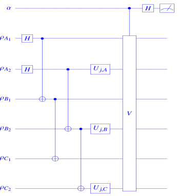
Figure 1: Overlap detection. Two copies $\rho^{p}_{A_{1}B_{1}C_{1}},\rho^{p}_{A_{2}B_{2}C_{2}}$ of a GHZ-diagonal state are prepared in the state $\rho_{i}=1/2(I_{2}+p\sigma_{z}),\forall i$. An Hadamard gate $H$ is applied to the qubits $A_{i},i=1,2$, followed by two CNOT gates on each copy. Then, one evaluates the purity and the overlap terms related to the observables $J_{3,x(y,z)}$, by applying the unitary transformations $U_{J_{3}}(\theta)=U_{j,A}(\theta)\otimes U_{j,B}(\theta)\otimes U_{j,C}(\theta),$ and measuring the ancilla polarisation by means of an interferometric scheme. This consists of an ancilla in the initial state $\alpha=1/\sqrt{2}(|0\rangle+|1\rangle)$ interacting with the two state copies by a controlled-$V$ gate, being $V$ the swap operator. A second Hadamard gate $H$ is finally applied to the ancilla. The mean value of the ancilla polarisation at the output is $\langle\sigma_{z}\rangle_{\alpha^{\text{out}}}=\text{Tr}[V\rho\otimes U_{J_{3}}(\theta)\rho U^{\dagger}_{J_{3}}(\theta)]=\text{Tr}[\rho U_{J_{3}}(\theta)\rho U^{\dagger}_{J_{3}}(\theta)]$, which determines the asymmetry lower bound.

As shown in Ref. me , the asymmetry lower bound is a function of mean values of self-adjoint operators. By applying the Taylor expansion about $\theta=\theta_{0}$, one has $\text{Tr}[\rho U_{H}(\theta)\rho U_{H}^{\dagger}(\theta)]=\text{Tr}[\rho U_{H}(\theta_{0})\rho U_{H}^{\dagger}(\theta_{0})]-(\text{Tr}[\rho^{2}H^{2}]-\text{Tr}[\rho H\rho H])(\theta-\theta_{0})^{2}+O((\theta-\theta_{0})^{3})$, and then ${\cal O}_{H}(\rho)\sim\frac{4}{(\theta-\theta_{0})^{2}}(\text{Tr}[\rho U_{H}(\theta_{0})\rho U_{H}^{\dagger}(\theta_{0})]-\text{Tr}[\rho U_{H}(\theta)\rho U_{H}^{\dagger}(\theta)]),\theta\rightarrow\theta_{0}$. By setting $\theta_{0}=0$, an approximation in terms of finite phase shifts, with error $O(\theta^{2})$, is given by ${\cal O}_{H}^{\text{ap}}(\rho)\pm\Delta{\cal O}_{H}^{\text{ap}}(\rho)$, with

$${\cal O}_{H}^{\text{ap}}(\rho) = 4\frac{\text{Tr}[\rho^{2}]-\text{Tr}[\rho U_{H}(\theta)\rho U_{H}^{\dagger}(\theta)]}{\theta^{2}},$$ (2)

$$\Delta{\cal O}_{H}^{\text{ap}}(\rho) = \underbrace{|d{{\cal O}_{H}^{\text{ap}}(\rho)}/d{\theta}|_{\theta=0}}_{=0}\theta+1/2|d^{2}{{\cal O}_{H}^{\text{ap}}(\rho)}/d{\theta}^{2}|_{\theta=0}\theta^{2}.$$

One may note that even the approximated quantity is a lower bound (but less tight) to the quantum Fisher information, ${\cal O}_{H}^{\text{ap}}(\rho)\leq{\cal O}_{H}(\rho),\forall\rho,H,\theta$ speed . Therefore, to quantify the lower bound to the asymmetry of the state, we need to evaluate its purity and the overlap with a second copy of the state after a rotation has been applied. They are obtained by estimating the mean value of the swap operator $V=\sum_{ij}|ij\rangle\langle ji|$ in two copies of the system, $\rho_{1,2}\equiv\rho$: $\text{Tr}[\rho^{2}]=\text{Tr}\Big{[}V(\rho\otimes\rho)\Big{]}$, while the overlap is given by $\text{Tr}\Big{[}\rho U_{H}\rho{U_{H}^{\dagger}}\Big{]}=\text{Tr}\Big{[}V\Big{(}\rho\otimes U_{H}\rho{U_{H}^{\dagger}}\Big{)}\Big{]}.$ Such quantities can be directly measured by implementing an interferometric configuration paz ; brun ; dariano ; ekertdir ; filip ; me ; jeong2 ; rugg . In fact, the method has general validity regardless the system state and the self-adjoint operator to be measured paz . Alternatively, for the relevant case of N-qubit systems, it is possible to extract purity and overlap by local Bell measurements, a routine measurement scheme in optical setups mintert ; mintert2 ; me ; pasca ; jeong2 ; geodiscordchina ; kus ; speed . Thus, for systems of arbitrary dimension, the lower bound $O_{H}(\rho)$ can be extracted by the statistics of a limited number of detections, bypassing full state reconstruction.

$J_{3}$	$J_{3,x}$	$J_{3,y}$	$J_{3,z}$
${\cal F}_{J_{3}}\left(\rho^{p}_{ABC}\right)$	$\frac{2p^{2}\left(p^{2}+2\right)}{p^{2}+1}$	$\frac{(-2p^{8}+p^{6}+18p^{4}+7p^{2})}{3p^{4}+4p^{2}+1}$	$(2p^{4}+4p^{3}+3p^{2})$
${\cal O}_{J_{3}}\left(\rho^{p}_{ABC}\right)$	$(2p^{2}+3p^{4}+p^{6})/2$	$(p^{6}+4p^{4}+7p^{2})/4$	$(3p^{6}+8p^{5}+14p^{4}+8p^{3}+3p^{2})/4$
${\cal F}_{J_{3}}\left(\rho^{p}_{ABC}\right)>3,5$	$p>1$	$p>1$	$p>0.674,0.813$
${\cal O}_{J_{3}}\left(\rho^{p}_{ABC}\right)>3,5$	$p>1$	$p>1$	$p>0.751,0.861$
${\cal\bar{F}}\left(\rho^{p}_{ABC}\right)>2,\bar{{\cal O}}\left(\rho^{p}_{ABC}\right)>2$	$p>0.646,0.772$

Table 1: Theoretical values of the quantum Fisher information, the observable lower bound defined in Eq. 1, and the conditions witnessing entanglement, Eq. 6, for the spin observables $J_{3,x(y,z)}$, in $\rho^{p}_{ABC}$. The coherence lower bound is an entanglement witness almost as efficient as the quantum Fisher information, being blind to entanglement only for $p\in[0.674,0.751],[0.646,0.772]$, and to tripartite entanglement for $p\in[0.813,0.861]$. Note that a more general sufficient condition for genuine tripartite entanglement is $|\rho_{1,8}|>\sqrt{\rho_{2,2}\,\rho_{7,7}}+\sqrt{\rho_{3,3}\,\rho_{6,6}}+\sqrt{\rho_{4,4}\,\rho_{5,5}}$, which for GHZ-diagonal states is also a necessary condition entsep . Hence, $\rho^{p}_{ABC}$ is three-partite entangled when $p>2^{2/3}-1\approx 0.587$.

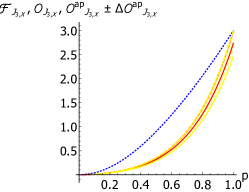
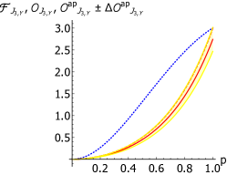
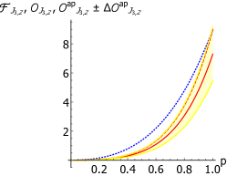
Figure 2: (Colors Online) – Evaluation of asymmetry in the state $\rho^{p}_{ABC}$ with respect to the observables $J_{3,x(y,z)}$ (figures (a), (b), and (c) respectively) as a function of the mixing parameter $p$. The blue dotted line is the quantum Fisher information, here showed for reference, the red dashed line is the bound ${\cal}O_{J_{3}}(\rho^{p}_{ABC})$, the red continuous line is the approximation ${\cal}O^{\text{ap}}_{J_{3}}(\rho^{p}_{ABC})$ obtained by imposing $\theta=\pi/6$, and the yellow band is the error region, whose extreme values are ${\cal}O^{\text{ap}}_{J_{3}}(\rho^{p}_{ABC})\pm\Delta{\cal}O^{\text{ap}}_{J_{3}}(\rho^{p}_{ABC})$.

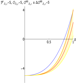
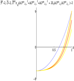
Figure 3: (Colors Online) – Witnessing entanglement by asymmetry via the inequalities in Eq. 6. (a) Witnessing entanglement in the state $\rho^{p}_{ABC}$ by computing the quantum Fisher information and the lower bound, as a function of the mixing parameter $p$. The blue dotted line depicts ${\cal F}_{J_{z,3}}(\rho^{p}_{ABC})-3$, the red dashed line is ${\cal O}_{J_{3,z}}(\rho^{p}_{ABC})-3$, while the red continuous line is ${\cal}O^{\text{ap}}_{J_{3}}(\rho^{p}_{ABC})-3$. Positive values of such quantities signal entanglement. The yellow band is the error region, bounded by the extreme values $({\cal O}^{\text{ap}}_{J_{3,z}}(\rho^{p}_{ABC})\pm\Delta{\cal O}^{\text{ap}}_{J_{3,z}}(\rho^{p}_{ABC}))-3$. The $J_{3,x(y)}$ cases are not reported as trivially useless, see Tab. 1. (b) Witnessing genuine tripartite entanglement (it is the case $N=3,k=2$ of Eq. 6). The blue dotted line depicts ${\cal F}_{J_{3,z}}(\rho^{p}_{ABC})-5$, the red dashed line is ${\cal O}_{J_{3,z}}(\rho^{p}_{ABC})-5$, while the red continuous line is ${\cal}O^{\text{ap}}_{J_{3}}(\rho^{p}_{ABC})-5$. The error region (yellow) is bounded by the extreme values of $({\cal O}^{\text{ap}}_{J_{3,z}}(\rho^{p}_{ABC})\pm\Delta{\cal O}^{\text{ap}}_{J_{3,z}}(\rho^{p}_{ABC}))-5$. (c) Witnessing entanglement by computing the average values of the quantum Fisher information and the lower bound over a spin basis $\{x,y,z\}$. The blue dotted line is $\bar{{\cal F}}(\rho^{p}_{ABC})-2$, the red dashed line is $\bar{{\cal O}}(\rho^{p}_{ABC})-2$, while the red continuous line is $\bar{{\cal O}}^{\text{ap}}_{J_{3}}(\rho^{p}_{ABC})-2$. The yellow error region is bounded by $\left(\bar{{\cal O}}^{\text{ap}}(\rho^{p}_{ABC})\pm\sqrt{\sum_{i}{\Delta{\cal O}^{\text{ap}}_{J_{3,i}}}^{2}(\rho^{p}_{ABC})+2\sum_{ij}\Delta{\cal O}^{\text{ap}}_{J_{3,i}}\Delta{\cal O}^{\text{ap}}_{J_{3,i}}}\right)-5$.

Closed formula for the asymmetry lower bound in multi-qubit systems

We here provide a closed formula for the asymmetry lower bound in one, two and three-qubit states, with respect to additive Hamiltonians $H_{N}=\sum_{i=1}^{N}h_{i},h_{i}=I_{1,2,\ldots,i-1}\otimes h_{i}\otimes I_{i+1,i+2,\ldots,N},h_{i}=1/2\sigma_{i}$, $\sigma_{i}$ representing spin-1/2 observables, e.g. the Pauli matrices. By recalling that $e^{i\sigma\theta/2}=\cos{\theta/2}~{}I_{2}+i\sin{\theta/2}~{}\sigma$, we get an exact expression for the lower bound in terms of phase shifts $U_{H_{N}}(\theta)=e^{-iH_{N}\theta}$. For $N=1,H_{1}=h$, one has

$${\cal O}_{H_{1}}(\rho) = \text{Tr}[\rho^{2}]-\text{Tr}[\rho U_{h}(\pi)\rho U_{h}^{\dagger}(\pi)],$$ (3)

For $N=2,H_{2}=h_{1}+h_{2}$:

$${\cal O}_{H_{2}}(\rho) = 3\text{Tr}[\rho^{2}]-4\text{Tr}[\rho U_{H_{2}}(\pi/2)\rho U_{H_{2}}^{\dagger}(\pi/2)]$$

$$+ \text{Tr}[\rho U_{H_{2}}(\pi)\rho U_{H_{2}}^{\dagger}(\pi)],$$

$$U_{H_{2}}(\theta) = U_{h_{1}}(\theta)U_{h_{2}}(\theta).$$ (4)

For $N=3,H_{3}=h_{1}+h_{2}+h_{3}$:

$${\cal O}_{H_{3}}(\rho) = 6\text{Tr}[\rho^{2}]-4\Big{\{}\text{Tr}[\rho U_{h_{1}+h_{2}}(\pi/2)\rho U_{h_{1}+h_{2}}^{\dagger}(\pi/2)]$$ (5)

$$+ \text{Tr}[\rho U_{h_{1}+h_{3}}(\pi/2)\rho U_{h_{1}+h_{3}}^{\dagger}(\pi/2)]$$

$$+ \text{Tr}[\rho U_{h_{2}+h_{3}}(\pi/2)\rho U_{h_{2}+h_{3}}^{\dagger}(\pi/2)]\Big{\}}$$

$$+ \text{Tr}[\rho U_{h_{1}+h_{2}}(\pi)\rho U_{h_{1}+h_{2}}^{\dagger}(\pi)]+\text{Tr}[\rho U_{h_{1}+h_{3}}(\pi)\rho U_{h_{1}+h_{3}}^{\dagger}(\pi)]$$

$$+ \text{Tr}[\rho U_{h_{2}+h_{3}}(\pi)\rho U_{h_{2}+h_{3}}^{\dagger}(\pi)]$$

$$+ \text{Tr}[\rho U_{h_{1}}(\pi)\rho U_{h_{1}}^{\dagger}(\pi)]+\text{Tr}[\rho U_{h_{2}}(\pi)\rho U_{h_{2}}^{\dagger}(\pi)]$$

$$+ \text{Tr}[\rho U_{h_{3}}(\pi)\rho U_{h_{3}}^{\dagger}(\pi)].$$

We conjecture that it is possible to iterate the procedure and work out equivalent expressions for an arbitrary number of qubits.

III Detection of multipartite entanglement via asymmetry

III.1 Asymmetry witnesses Entanglement

It is often desirable to consider a high dimensional system as a partition of subsystems. Such a partition is usually dictated by the physical constraints of the problem, for example the spatial separation between the parts of the system. It is then interesting to understand the interplay between asymmetry with respect to a global observable and the quantum properties of the subsystems. In spite of being a basis-dependent feature, coherence is linked to basis-independent features of multipartite systems as quantum correlations lqu ; ger2 ; china ; alta ; morimae . Here we show that, for an $N$-qubit system, the observable asymmetry bound ${\cal O}_{H}(\rho)$ measured on the global system state witnesses entanglement between the partitions. There are several entanglement witnesses written in terms of the quantum Fisher information. They relate entanglement to the system speed of response to phase shifts generated by additive spin-$1/2$ Hamiltonians $J_{N}=\sum_{i=1}^{N}1/2\sigma_{i}$ toth ; toth2 ; toth4 ; smerzi ; smerzi2 . In particular, a constraint which cannot be satisfied by $k$-separable states of $N$ qubits is ${\cal F}_{J_{N}}(\rho)\geq nk^{2}+(N-nk)^{2}$, where $n=\lfloor\frac{N}{k}\rfloor$. Thus, verifying this relation certifies genuine $k$-partite entanglement horo . Also, if $\bar{{\cal F}}(\rho)=1/3({\cal F}_{J_{N,x}}(\rho)+{\cal F}_{J_{N,y}}(\rho)+{\cal F}_{J_{N,z}}(\rho))>2N/3$, then the state is entangled. Therefore, if there exists a spin basis $\{x,y,z\}$ such that the following conditions are satisfied:

$${\cal O}_{J_{N,x(y,z)}}(\rho) > nk^{2}+(N-nk)^{2},$$ (6)

$$\bar{\cal O}(\rho) = 1/3({\cal O}_{J_{N,x}}(\rho)+{\cal O}_{J_{N,y}}(\rho)+{\cal O}_{J_{N,z}}(\rho))>2N/3,$$

a state $\rho$ is respectively genuinely $k$-partite entangled and entangled.

III.2 A case study

Here we apply our scheme to simulate the non-tomographic detection of asymmetry and entanglement in a three-qubit state. We choose as probe state the GHZ-diagonal state $\rho^{p}_{\text{ABC}}$. This allows one to investigate the behavior of the asymmetry lower bound and entanglement witness in the presence of noise in the system. The two copies of the GHZ diagonal state $\rho^{p}_{A_{1}B_{1}C_{1}},\rho^{p}_{A_{2}B_{2}C_{2}}$ are obtained by initializing a six qubit processor in $\rho_{i}=1/2(I_{2}+p\sigma_{z}),i=i\ldots,6$, and applying Hadamard and CNOT gates as described in Fig. 1.
We measure the asymmetry of the input state with respect to the set of spin Hamiltonians $J_{3}=\sum_{i=A,B,C}j_{3,i},j_{3,A}=j_{A}\otimes I_{BC},j_{3,B}=I_{A}\otimes j_{B}\otimes I_{C},j_{3,C}=I_{AB}\otimes j_{C},j=1/2\sigma_{x,(y,z)},$ by computing the values of the lower bound, and the approximation defined in Eq. 2, for each observable. Of course, we may obtain the asymmetry with respect to any self-adjoint operator in the three-qubit Hilbert space. This is done by implementing the unitary gate $U_{J_{3}}(\theta)=U_{j,A}(\theta)\otimes U_{j,B}(\theta)\otimes U_{j,C}(\theta)$ on a copy of the state and then building up an interferometric configuration (Fig. 1). Performing the polarisation measurements on the ancillary qubit makes possible to determine ${\cal O}_{J_{3}}(\rho^{p}_{ABC})$. We select a small but experimentally plausible phase shift, $\theta=\pi/6$ speed . Obviously, to evaluate the purity, no gate has to be applied. The purity and overlap values extracted by the quantities $\text{Tr}[\rho^{p}_{ABC}U_{J_{3}}(\pi/6)\rho^{p}_{ABC}U_{J_{3}}^{\dagger}(\pi/6)]$ determine ${\cal O}_{J_{3}}^{\text{ap}}(\rho^{p}_{ABC})$. No further action is necessary to verify the presence of entanglement through the witnesses in Eq. 6, as the values of ${\cal O}^{\text{ap}}_{J_{3}}(\rho^{p}_{ABC})$ have been obtained in the previous steps. For $N=3$, we have $k=1\Rightarrow{\cal O}_{J_{3}}(\rho^{p}_{ABC})\geq 3,k=2\Rightarrow{\cal O}_{J_{3}}(\rho^{p}_{ABC})\geq 5,$ and ${\cal\bar{O}}(\rho^{p}_{ABC})>2$. The results are summarised in Tab. 1 and Figs. 3,3.

IV Conclusion

In this work, we provided an experimental recipe to witness multipartite entanglement by detecting asymmetry with respect to an additive Hamiltonian. We employed an experimentally friendly lower bound of the quantum Fisher information to quantify asymmetry, a geometric property of quantum systems underpinned by coherence in an observable eigenbasis. The scheme is suitable for detection of asymmetry in large scale quantum registers, as it requires a limited number of measurements regardless the dimension of the system. We showed that in multipartite states the asymmetry lower bound with respect to additive observables is a witness of multipartite entanglement. Our results suggest further lines of investigation. To the best of our knowledge, the lower bound ${\cal O}_{H}$ is the first faithful experimental quantifier of asymmetry for finite dimensional systems. Thus, on the experimental side, we call for a demonstration of our study. Moreover, we observe that a quadratic ($O(N^{2})$) sensitivity to phase shifts generated by additive Hamiltonian in $N$-party systems, as measured by the quantum Fisher information, has been associated to another elusive quantum effect, i.e. quantum macroscopicity leggett ; frow ; ben . It is clear that high values of coherence are essential to quantum macroscopicity, yet the interplay between the two concepts still needs to be clarified.

References

• (1) M. Horodecki and J. Oppenheim, Int. J. Mod. Phys. B 27, 1345019 (2013).
• (2) S. D. Bartlett, T. Rudolph, and R. W. Spekkens, Rev. Mod. Phys. 79, 555 (2007).
• (3) G. Gour and R.W. Spekkens, New J. Phys. 10, 033023 (2008).
• (4) I. Marvian, Symmetry, Asymmetry and Quantum Information, Phd Thesis, University of Waterloo (2012).
• (5) M. Ahmadi, D. Jennings, and T. Rudolph, New J. Phys. 15, 013057 (2013).
• (6) D. Girolami, T., Tufarelli, and G. Adesso, Phys. Rev. Lett. 110, 240402 (2013).
• (7) I. Marvian and R. W. Spekkens, Nature Comm. 5, 3821 (2014).
• (8) D. Girolami, Phys. Rev. Lett. 113, 170401 (2014).
• (9) D. Girolami et al., Phys. Rev. Lett 112, 210401 (2014).
• (10) S. Luo, Phys. Rev. Lett. 91, 180403 (2003).
• (11) J. Aberg, Phys. Rev. Lett. 113, 150402 (2014).
• (12) S. Luo, Theor. Math. Phys. 143, 681 (2005).
• (13) S. Luo, S. Fu, and C. H. Oh, Phys. Rev. A 85, 032117 (2012).
• (14) F. Herbut, J. of Phys. A 38, 2959 (2005).
• (15) T. Baumgratz, M. Cramer, and M. B. Plenio, Phys. Rev. Lett. 113, 140401 (2014).
• (16) Y. Yao, X. Xiao, L. Ge, and C. P. Sun, Phys. Rev. A 92, 022112 (2015).
• (17) S. Du, Z. Bai, and Y, Guo, Phys. Rev. A 91, 052120 (2015).
• (18) A. Streltsov, U. Singh, H. S. Dhar, M. N. Bera, and G. Adesso, Phys. Rev. Lett. 115, 020403 (2015).
• (19) Z. Xi, Y. Li, and H. Fan, Sci. Rep. 5, 10922 (2015).
• (20) C.-M. Li, N. Lambert, Y.-N. Chen, G.-Y. Chen, and F. Nori, Sci. Rep. 2, 885 (2012).
• (21) A. Monras, A. Checinska, and A. K. Ekert, New J. Phys. 16, 063041 (2014).
• (22) F. A. Pollock, A. Checinska, S. Pascazio, and K. Modi, arXiv:1507.05051.
• (23) C. Altafini, Phys. Rev. A 012311 (2004).
• (24) T. R. Bromley, M. Cianciaruso, and G. Adesso, Phys. Rev. Lett. 114, 210401 (2015).
• (25) R. Horodecki, P. Horodecki, M. Horodecki, and K. Horodecki, Rev. Mod. Phys. 81, 865 (2009).
• (26) R. Jozsa and N. Linden, Proc. R. Soc. Lon A. 459, 2011 (2003).
• (27) V. Giovannetti, S. Lloyd, and L. Maccone, Nature Photon. 5, 222 (2011).
• (28) A. Shimizu and T. Morimae, Phys. Rev. Lett. 95, 090401 (2005).
• (29) M. Huber, F. Mintert, A. Gabriel and B. C. Hiesmayer, Phys. Rev. Lett. 104, 210501 (2010).
• (30) O. Gühne and G. Tóth, Phys. Rep. 474, 1 (2009).
• (31) C. W. Helstrom, Quantum detection and estimation theory (Academic Press, New York, 1976).
• (32) G. Tóth and I. Apellaniz, J. Phys. A: Math. Theor. 47, 424006 (2014).
• (33) C. Zhang, et al., arXiv:1611.02004.
• (34) J. P. Paz and A. Roncaglia, Phys. Rev. A 68, 052316 (2003).
• (35) T. A. Brun, Quant. Inf. and Comp. 4, 401 (2004).
• (36) G. M. D’Ariano and P. Perinotti, Phys. Rev. Lett. 94, 090401 (2005).
• (37) A. K. Ekert, C. Moura Alves, D. K. L. Oi, M. Horodecki, P. Horodecki, and L. C. Kwek, Phys. Rev. Lett. 88, 217901 (2002).
• (38) R. Filip, Phys. Rev. A 65, 062320 (2002).
• (39) H. Jeong, C. Noh, S. Bae, D. G. Angelakis, and T. C. Ralph, J. Opt. Soc. Am. B 31, 3057 (2014).
• (40) H. Nakazato, T. Tanaka, K. Yuasa, G. Florio, and S. Pascazio, Phys. Rev. A 85, 042316 (2012).
• (41) F. Mintert and A. Buchleitner, Phys. Rev. Lett. 98, 140505 (2007).
• (42) S. P. Walborn, P. H. Souto Ribeiro, L. Davidovich, F. Mintert, and A. Buchleitner, Nature 440, 1022 (2006).
• (43) M. Oszmaniec and M. Kuś Phys. Rev. A 88, 052328 (2013).
• (44) J. Jin, F. Zhang, C. Yu, and H. Song J. Phys. A: Math. Theor. 45, 115308 (2012).
• (45) S. Yu, arXiv:1302.5311.
• (46) G. Tóth and D. Petz, Phys. Rev. A 87, 032324 (2013).
• (47) D. Petz, Lin. Alg. Appl. 244, 81 (1996).
• (48) P. Gibilisco, D. Imparato, and T. Isola, Proc. of the Am. Math. Soc. 137, 317 (2008).
• (49) D. Paiva Pires, L. C. Céleri, and D. O. Soares-Pinto, Phys. Rev. A 91, 042330 (2015).
• (50) X. Wang and S. G. Schirmer, Phys. Rev. A 79, 052326 (2009).
• (51) T. Tufarelli, D. Girolami, R. Vasile, S. Bose, and G. Adesso, Phys. Rev. A 86, 052326 (2012).
• (52) M. Piani, Phys. Rev. A 86, 034101 (2012).
• (53) D. Girolami, R. Vasile, and G. Adesso, Int. J. of Mod. Phys. B 27, 1345020 (2013).
• (54) L. Pezzé and A. Smerzi, Phys. Rev. Lett. 110, 163604 (2013).
• (55) G. Tóth, Phys. Rev. A 85, 022322 (2012).
• (56) P. Hyllus, W. Laskowski, R. Krischek, C. Schwemmer, W. Wieczorek, H. Weinfurter, L. Pezzé, and A. Smerzi, Phys. Rev. A 85, 022321 (2012).
• (57) O. Gühne and M. Seevinck, New J. Phys. 12, 053002 (2010).
• (58) A. Leggett, Prog. Theor. Phys. Supp. 69, 80 (1980).
• (59) F. Fröwis and W. Dür, New J. Phys. 14, 093039 (2012).
• (60) B. Yadin and V. Vedral, Phys. Rev. A 93, 022122 (2016).