Black holes and wormholes subject to conformal mappings

Abstract

Solutions of the field equations of theories of gravity which admit distinct conformal frame representations can look very different in these frames. We show that Brans class IV solutions describe wormholes in the Jordan frame (in a certain parameter range) but correspond to horizonless geometries in the Einstein frame. The reasons for such a change of behaviour under conformal mappings are elucidated in general, using Brans IV solutions as an example.

I Introduction

Conformal transformations are widely used in General Relativity Waldbook and especially in alternative theories of gravity BD61 ; FujiiMaeda ; mybook ; CapozzielloFaraonibook . Scalar-tensor and $f(R)$ gravity (which can be reduced to the former reviews ) can be represented in infinitely many conformal frames, of which the Jordan and the Einstein frame are commonly used FujiiMaeda ; mybook . By conformally transforming a black hole, often the result is not another black hole geometry. Other times, a horizonless geometry (possibly containing a naked singularity) is conformally transformed to a black hole solution of the field equations or even to a wormhole and, vice-versa, a black hole can be transformed into a naked singularity. Although this phenomenology has been noted occasionally in the literature (e.g., noted1 ; noted2 ; noted3 ; Alex ), to the best of our knowledge it has not been investigated. Here we fill this gap by tracing the cause of the disappearance of horizons and the appearance of new ones under the action of conformal transformations. For concreteness, we apply our discussion to scalar-tensor gravity, but the context is more general and our results can be applied to any situation in which a spacetime metric is conformally transformed, including in General Relativity. For simplicity, however, we consider spherically symmetric metrics and we provide an example which is, in addition, static.

In the course of our discussion we elucidate (Sec. II) the nature of the well known Brans class IV solutions of Brans-Dicke gravity, which constitute our example for the general problem. For a certain range of parameters, they are found to represent asymptotically flat wormholes with a horizon, while for other parameter ranges they are horizonless geometries hosting naked singularities. This radical change in geometry is not limited to this example but occurs frequently when conformal mappings of spacetime metrics are involved, not only in scalar-tensor gravity but also in General Relativity. The reasons for such a change in geometry are investigated and clarified in Sec. III for general situations.

We remind the reader that the (Jordan frame) action of scalar-tensor gravity is

$$S_{\text{ST}} = \int d^{4}x\sqrt{-g}\left[\frac{1}{16\pi}\left(\phi{\cal R}-\frac{\omega(\phi)}{\phi}\,\nabla^{a}\phi\nabla_{a}\phi\right)-V(\phi)\right.$$ (1)

$$\left.+{\cal L}_{\text{matter}}\right]\,,$$

where ${\cal R}$ is the Ricci curvature of spacetime, $g$ is the determinant of the spacetime metric $g_{ab}$, and $\phi$ is the Brans-Dicke-like scalar field, while $V(\phi)$ is a scalar field potential. A conformal transformation of the metric $g_{ab}\rightarrow\tilde{g}_{ab}=\Omega^{2}g_{ab}$ with conformal factor $\Omega=\sqrt{\phi}$, together with the scalar field redefinition

$$d\tilde{\phi}=\sqrt{\frac{|2\omega(\phi)+3|}{16\pi}}\,\frac{d\phi}{\phi}$$ (2)

recasts the theory in its Einstein frame form

$$S_{\text{ST}} = \int d^{4}x\sqrt{-\tilde{g}}\left[\frac{\cal R}{16\pi}-\frac{1}{2}\,\tilde{g}^{ab}\nabla_{a}\tilde{\phi}\nabla_{b}\tilde{\phi}-U\left(\tilde{\phi}\right)\right.$$ (3)

$$\left.+\frac{{\cal L}_{\text{matter}}}{\left(\phi(\tilde{\phi})\right)^{2}}\right]$$

in which the gravity sector looks like General Relativity and the new scalar field $\tilde{\phi}$ couples minimally to gravity (but non-minimally to matter) and has canonical kinetic energy density and potential

$$U\left(\tilde{\phi}\right)=\frac{V\left(\phi(\tilde{\phi})\right)}{\left(\phi(\tilde{\phi})\right)^{2}}\,.$$ (4)

We use units in which Newton’s constant $G$ and the speed of light $c$ are unity, the metric signature is $-+++$, and we follow the notations and conventions of Ref. Waldbook .

II Brans class IV solutions

Brans class IV spacetimes Brans62 form an often quoted class of static and spherically symmetric solutions of vacuum Brans-Dicke theory (without scalar field potential). Class III and class IV solutions Brans62 can be obtained from each other by means of a mathematical transformation involving the radial coordinate and the parameters BhadraNandi2001 ; BhadraSarkarGRG2005 . Although the discovery of these solutions was made only one year after the introduction of Brans-Dicke theory Brans62 , and often cited, they are still not well uderstood.

The line element and Brans-Dicke scalar field in isotropic coordinates in the Jordan frame are Brans62

$$ds^{2}=-\mbox{e}^{2\alpha_{0}-\frac{2}{B_{0}\varrho}}dt^{2}+\mbox{e}^{2\beta_{0}+\frac{2(C_{0}+1)}{B_{0}\varrho}}\left(d\varrho^{2}+\varrho^{2}d\Omega_{(2)}^{2}\right)\,,$$ (5)

$$\phi(\varrho)=\phi_{0}\,\mbox{e}^{-\frac{C_{0}}{B_{0}\varrho}}\,,$$ (6)

where $d\Omega_{(2)}^{2}=d\theta^{2}+\sin^{2}\theta\,d\varphi^{2}$ is the line element on the unit 2-sphere and

$$C_{0}=\frac{-1\pm\sqrt{-2\omega-3}}{\omega+2}$$ (7)

(which requires that $2\omega+3\leq 0$), and where $\alpha_{0},\beta_{0},B_{0},C_{0}$, and $\phi_{0}$ are constants. The factors $\mbox{e}^{2\alpha_{0}}$ and $\mbox{e}^{2\beta_{0}}$ can be absorbed by rescaling the coordinates $t$ and $\varrho$, respectively, and in the following they are dropped.

A notable feature of Brans class IV solutions is that, as the Brans-Dicke parameter $\omega\rightarrow-\infty$, they do not reduce to the corresponding vacuum solution of General Relativity, the Schwarzschild solution, but to

$$ds^{2}\approx-\mbox{e}^{-\frac{2}{B_{0}\varrho}}dt^{2}+\mbox{e}^{\frac{2}{B_{0}\varrho}}\left(d\varrho^{2}+\varrho^{2}d\Omega_{(2)}^{2}\right)\,,$$ (8)

$$\phi(\varrho)\approx\phi_{0}\,.$$ (9)

This anomalous behaviour is related to the fact that the scalar $\phi$ does not have the usual Weinberg asymptotic behaviour $\phi=\phi_{0}+\frac{\phi_{1}}{\omega}+\frac{\phi_{2}}{\omega^{2}}+\,...$ as $|\omega|\rightarrow+\infty$, but rather follows $\phi=\phi_{0}+\mbox{O}\left(1/\sqrt{|\omega|}\right)$. It is well known that Brans class I solutions exhibit the same phenomenon RomeroBarros ; BanerjeeSen ; VFlimit ; BhadraNandilimit , so the lack of a limit to General Relativity for class IV solutions is not a surprise.

The areal radius of the Brans class IV geometry (5) is

$$R(\varrho)=\mbox{e}^{\frac{C_{0}+1}{B_{0}\varrho}}\,\varrho\,.$$ (10)

Let us see how 2-spheres of symmetry behave as the isotropic radius $\varrho$ varies. We have

$$\frac{dR}{d\varrho}=\mbox{e}^{\frac{C_{0}+1}{B_{0}\varrho}}\left(1-\frac{\varrho_{0}}{\varrho}\right)$$ (11)

where

$$\varrho_{0}\equiv\frac{C_{0}+1}{B_{0}}\,.$$ (12)

Assuming $\omega<-3/2$ and $B_{0}\neq 0$, we consider separately three possible parameter ranges which we present in Fig. 1.

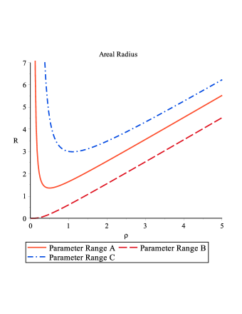
Figure 1: The areal radius $R(\varrho)$ for the three ranges of values of the parameters $B_{0}$ and $C_{0}$ considered in the text. We use $(B_{0},C_{0})=(1,-1/2)$, $(-1,-1/2)$ and $(-1,1.9)$ for parameter ranges A, B and C, respectively.

II.1 Parameter range $B_{0}>0,\,C_{0}>-1$

In this case it is $dR/d\varrho\geq 0$ for $\varrho\geq\varrho_{0}$ and this derivative is negative otherwise: the areal radius $R(\varrho)$ diverges as $\varrho\rightarrow 0^{+}$, decreases as $\varrho$ increases, assumes a global minimum $R_{\text{min}}=\mbox{e}\varrho_{0}$ at $\varrho_{0}$, and increases to $+\infty$ as $\varrho\rightarrow+\infty$. There are, therefore, two branches of the areal radius $R$ as $\varrho$ varies in the range $0\leq\varrho<+\infty$. In order to understand what happens at $\varrho_{0}$, we rewrite the line element (5) using the areal radius instead of the coordinate $\varrho$, which gives straightforwardly

$$ds^{2}=-\mbox{e}^{-\frac{2}{B_{0}\varrho}}dt^{2}+\frac{dR^{2}}{\left(1-\varrho_{0}/\varrho\right)^{2}}+R^{2}d\Omega_{(2)}^{2}\,.$$ (13)

The apparent/trapping horizons (if any exist) of any spherically symmetric metric are located at the roots of the equation $\nabla^{c}R\nabla_{c}R=0$ NielsenVisser ; AbreuVisser ; VFhorizons which, in these coordinates, correspond to $g^{RR}=0$ or $\left(1-\varrho_{0}/\varrho\right)^{2}=0$, which has $\varrho_{0}$ as a double root. Here, $g^{RR}$ does not change sign at the minimum $R_{\text{min}}$. In general wherever $g^{RR}$ changes sign, so that $\partial g^{RR}/\partial R\neq 0$ there and $g^{RR}$ has a single root, there exists a black hole horizon. In this black hole case, the isotropic radius $\varrho>0$ corresponds to a double covering of the exterior region Buchdhal . Therefore, for the range of parameters we are considering here, $\varrho=\varrho_{0}$ corresponds to an horizon, but not to a black hole horizon: the line element (5) corresponds to a wormhole with the two throats joining at the horizon. This conclusion is similar to that reached in Ref. Vanzoetal2012 for the Campanelli-Lousto spacetimes CampanelliLousto , another class of static and spherically symmetric solutions of Brans-Dicke theory which are often (erroneously) referred to as black holes.

The Ricci, Ricci squared, and Kretschmann scalars are

$${\cal R} = \frac{2}{R^{2}}\left[1-\left(1-\frac{\varrho_{0}}{\varrho}\right)^{2}\right]\,,$$ (14)

$$R_{ab}R^{ab} = \frac{2}{R^{4}}\left[1-\left(1-\frac{\varrho_{0}}{\varrho}\right)^{2}\right]^{2}\,,$$ (15)

$$R_{abcd}R^{abcd} = \frac{4}{R^{4}}\left[1-\left(1-\frac{\varrho_{0}}{\varrho}\right)^{2}\right]^{2}\,,$$ (16)

respectively. These scalars do not diverge since $R$ stops at its minimum $R_{\text{min}}$ and does not reach zero value.

II.2 Parameter range $B_{0}<0,C_{0}>-1$

For the parameter values $B_{0}<0,\,C_{0}>-1$, it is $\varrho_{0}\equiv\frac{C_{0}+1}{B_{0}}<0$ and $dR/d\varrho>0$ for any positive value of $\varrho$, hence the areal radius has no positive minimum. The function $R(\varrho)$ increases monotonically from $R(0)=0$ to positive infinity as $\varrho$ increases. In this case there are no horizons. All the scalar invariants (14)-(16) diverge as $R\rightarrow 0$ (corresponding to $\varrho\rightarrow 0$). This spacetime harbours a naked singularity at $R=0$.

II.3 Parameter range $B_{0}<0,\,C_{0}<-1$

For this value of the parameters it is again $\varrho_{0}=\left|\frac{C_{0}+1}{B_{0}}\right|>0$ and the function $R(\varrho)$ is again decreasing for $0\leq\varrho<\varrho_{0}$, minimum at $\varrho_{0}$, and increasing for $\varrho>\varrho_{0}$. We have again two wormhole throats joining at an horizon located at $R_{\text{min}}$ and no spacetime singularities are present.

II.4 Einstein frame Brans IV metric

Let us consider now, for all values of the parameters $B_{0}$ and $C_{0}$, the Einstein frame version of Brans-Dicke theory. By performing the usual conformal rescaling of the metric to the Einstein frame

$$g_{ab}\rightarrow\tilde{g}_{ab}=\Omega^{2}g_{ab}\,,\;\;\;\;\;\Omega=\sqrt{\phi}$$ (17)

and the nonlinear scalar field redefinition

$$\phi\rightarrow\tilde{\phi}=\sqrt{\frac{|2\omega+3|}{16\pi}}\,\ln\left(\frac{\phi}{\phi_{*}}\right)$$ (18)

where $\phi_{*}$ is a constant, the theory is recast in the form of Einstein gravity with a minimally coupled scalar field. Dropping irrelevant constants, one obtains the Einstein frame line element and scalar field

$$d\tilde{s}^{2}=-\mbox{e}^{-\frac{(C_{0}+2)}{B_{0}\varrho}}dt^{2}+\mbox{e}^{\frac{C_{0}+2}{B_{0}\varrho}}\left(d\varrho^{2}+\varrho^{2}d\Omega_{(2)}^{2}\right)\,,$$ (19)

$$\tilde{\phi}=\phi_{1}-\frac{\phi_{2}}{\varrho}\,,$$ (20)

where

$$\phi_{1} = \sqrt{\frac{|2\omega+3|}{16\pi}}\,\ln\left(\frac{\phi}{\phi_{*}}\right)\,,$$ (21)

$$\phi_{2} = -\sqrt{\frac{|2\omega+3|}{16\pi}}\,\frac{C_{0}}{B_{0}}\,.$$ (22)

Now the areal radius is not given by (10) but by

$$\tilde{R}=\mbox{e}^{\frac{C_{0}+2}{2B_{0}\varrho}}\,\varrho$$ (23)

which differs from its Jordan frame counterpart in the numerical coefficient of $1/(B_{0}\varrho)$ in the exponent. The same analysis performed in the Jordan frame can be repeated here but now the critical isotropic radius is not $\varrho_{0}$ but

$$\tilde{\varrho}_{0}\equiv\frac{C_{0}+2}{2B_{0}}=\frac{\varrho_{0}}{2}+\frac{1}{2B_{0}}\,.$$ (24)

Assuming $B_{0}>0$, one immediately sees that

1. $\tilde{\varrho}_{0}>\varrho_{0}$ if $-1<C_{0}<0$;

2. $\tilde{\varrho}_{0}<\varrho_{0}$ if $C_{0}>0$;

3. but $\tilde{\varrho}_{0}>0$ and $\varrho_{0}<0$ for $-2<C_{0}<-1$.

These three scenarios are indicated in Fig. 2.

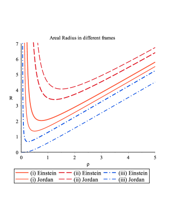
Figure 2: Einstein frame and Jordan frame areal radius for the three scenarios described in the text.

Consider the parameter range (iii) given by $B_{0}>0$ and $-2<C_{0}<-1$ which is plotted in the blue dash-dotted curves in Fig. 2: in the Einstein frame the Brans IV solution describes a wormhole while in the Jordan frame, for the same parameter range, it describes a horizonless geometry. The reason for this change introduced by the conformal transformation is discussed in Sec. IV. The Ricci, Ricci squared, and Kretschmann scalars in the Einstein frame are

$$\tilde{{\cal R}} = \frac{2\,\mbox{e}^{\frac{-2\left(C_{0}+2\right)}{B_{0}\varrho}}}{\varrho^{2}}=\frac{2}{\tilde{R}^{2}}\,,$$ (25)

$$\tilde{R}_{ab}\tilde{R}^{ab} = \frac{1}{2}\,\tilde{R}_{abcd}\tilde{R}^{abcd}=\frac{2\,\mbox{e}^{\frac{-2\left(C_{0}+2\right)}{B_{0}\varrho}}}{\varrho^{4}}\,,$$ (26)

and are regular in the parameter range $B_{0}>0$ and $-2<C_{0}<-1$ since the coordinate $\varrho$ does not go below the minimum value $\tilde{\varrho}_{0}$.

III The general problem

Let us consider now the general problem: how can it happen that a geometry without horizons, when conformally transformed, becomes a black hole or a wormhole? Surely something so physically dramatic as a horizon does not depend crucially on an overall factor in the metric! The answer is that there is no straightforward relation between (apparent) horizons in one geometry and (apparent) horizons of the conformally transformed metric, or even between the numbers of horizons present. Null geodesics, the causal structure of spacetime and event horizons (which are null surfaces) are conformally invariant, but apparent and trapping horizons are spacelike or timelike surfaces and therefore they are affected by a conformal transformation.

Let us restrict, for simplicity, to spherically symmetric metrics, the line element of which can generically be written as

$$ds^{2}=-A(t,R)dt^{2}+B(t,R)dR^{2}+R^{2}d\Omega_{(2)}^{2}\,.$$ (27)

This line element is not required to be stationary and, clearly, $R$ is the areal radius. The apparent horizons, if they exist, are located by the equation $g^{RR}=1/B(t,R)=0$ (which may or may not have roots). In addition, in order to have a black hole and not a wormhole it is required that $g^{RR}$ have single roots, that is, $\partial g^{RR}/\partial R\neq 0$ where $g^{RR}$ vanishes.

The conformally transformed geometry is given by

$$d\tilde{s}^{2}=-\Omega^{2}Adt^{2}+\Omega^{2}BdR^{2}+\tilde{R}^{2}d\Omega_{(2)}^{2}\,,$$ (28)

where $\Omega=\Omega(t,R)$ to preserve the spherical symmetry and $\tilde{R}=\Omega(t,R)R$ is the areal radius in the conformally transformed world.

One rewrites the “new” metric (28) in the form (27) as

$$d\tilde{s}^{2}=-\tilde{A}(\tilde{t},\tilde{R})d\tilde{t}^{2}+\tilde{B}(\tilde{t},\tilde{R})d\tilde{R}^{2}+\tilde{R}^{2}d\Omega_{(2)}^{2}\,,$$ (29)

where $\tilde{t}$ is a suitable time coordinate and $\tilde{R}$ is the areal radius in the Einstein frame. The form of the functions $\tilde{A}(\tilde{t},\tilde{R})$ and $\tilde{B}(\tilde{t},\tilde{R})$ was computed in Ref. ValerioEnzo2013 , which we follow here.

The use of the relation

$$dR=\frac{d\tilde{R}-\Omega_{,t}Rdt}{\Omega_{,R}R+\Omega}$$ (30)

in the line element (28) provides

$$d\tilde{s}^{2} = -\left[\Omega^{2}A-\frac{\Omega_{,t}^{2}R^{2}\Omega^{2}B}{\left(\Omega_{,R}R+\Omega\right)^{2}}\right]dt^{2}$$ (31)

$$+\frac{\Omega^{2}B}{\left(\Omega_{,R}R+\Omega\right)^{2}}\,d\tilde{R}^{2}$$

$$-\,\frac{2\Omega^{2}\Omega_{,t}BR}{\left(\Omega_{,R}R+\Omega\right)^{2}}\,dtd\tilde{R}+\tilde{R}^{2}d\Omega_{(2)}^{2}\,.$$

The $dt\,d\tilde{R}$ cross-term can be removed by the use of a new time coordinate $\tilde{t}(t,R)$ which satisfies

$$d\tilde{t}=\frac{1}{F}\left(dt+\beta dR\right)\,,$$ (32)

with $\beta\left(t,R\right)$ an unknown function to be determined and $F\left(t,R\right)$ an integrating factor which necessarily obeys the differential relation

$$\frac{\partial}{\partial R}\left(\frac{1}{F}\right)=\frac{\partial}{\partial t}\left(\frac{\beta}{F}\right)$$ (33)

which ensures that $d\tilde{t}$ is an exact differential. Substitution of $dt=Fd\tilde{t}-\beta d\tilde{R}$ into the line element yields

$$d\tilde{s}^{2} = -\left[\Omega^{2}A-\frac{\Omega_{,t}^{2}R^{2}\Omega^{2}B}{\left(\Omega_{,R}R+\Omega\right)^{2}}\right]F^{2}d\tilde{t}^{2}+\left\{-\beta^{2}\left[\Omega^{2}A-\frac{\Omega_{,t}^{2}R^{2}\Omega^{2}B}{\left(\Omega_{,R}R+\Omega\right)^{2}}\right]+\frac{\Omega^{2}B}{\left(\Omega_{,R}R+\Omega\right)^{2}}\right.$$ (34)

$$\left.+\frac{2\beta\Omega_{,t}\Omega^{2}BR}{\left(\Omega_{,R}R+\Omega\right)^{2}}\right\}d\tilde{R}^{2}+2F\left\{\beta\left[\Omega^{2}A-\frac{\Omega_{,t}^{2}R^{2}\Omega^{2}B}{\left(\Omega_{,R}R+\Omega\right)^{2}}\right]-\frac{\Omega_{,t}\Omega^{2}RB}{\left(\Omega_{,R}R+\Omega\right)^{2}}\right\}d\tilde{t}\,d\tilde{R}+\tilde{R}^{2}d\Omega_{(2)}^{2}\,.$$

We now fix the function $\beta$ as

$$\beta\left(t,R\right)=\frac{\Omega_{,t}\Omega^{2}BR}{\left[\Omega^{2}A-\frac{\Omega_{,t}^{2}R^{2}\Omega^{2}B}{\left(\Omega_{,R}R+\Omega\right)^{2}}\right]\left(\Omega_{,R}R+\Omega\right)^{2}}$$ (35)

and the line element is diagonalized:

$$d\tilde{s}^{2} = -\left[\Omega^{2}A-\frac{\Omega_{,t}^{2}\Omega^{2}BR^{2}}{\left(\Omega_{,R}R+\Omega\right)^{2}}\right]F^{2}d\tilde{t}^{2}+\frac{\Omega^{2}B}{\left(\Omega_{,R}R+\Omega\right)^{2}}\cdot\left\{1+\frac{\Omega_{,t}^{2}\Omega^{2}BR^{2}}{\left(\Omega_{,R}R+\Omega\right)^{2}\left[\Omega^{2}A-\frac{\Omega_{,t}^{2}\Omega^{2}BR^{2}}{\left(\Omega_{,R}R+\Omega\right)^{2}}\right]}\right\}d\tilde{R}^{2}$$ (36)

$$+\tilde{R}^{2}d\Omega_{(2)}^{2}\,.$$

By comparing eqs. (36) and (29) one obtains

$$\tilde{A} = \left[\Omega^{2}A-\frac{\Omega_{,t}^{2}\Omega^{2}BR^{2}}{\left(\Omega_{,R}R+\Omega\right)^{2}}\right]F^{2}\,,$$ (37)

$$\tilde{B} = \left.\frac{B\Omega^{2}}{\left(\Omega_{,R}R+\Omega\right)^{2}}\right\{1$$ (38)

$$\left.+\frac{\Omega_{,t}^{2}\Omega^{2}BR^{2}}{\left(\Omega_{,R}R+\Omega\right)^{2}\left[\Omega^{2}A-\frac{\Omega_{,t}^{2}\Omega^{2}BR^{2}}{\left(\Omega_{,R}R+\Omega\right)^{2}}\right]}\right\}\,.$$

the equation locating the apparent horizons of the tilded geometry is now $1/\tilde{B}=0$. Restricting to static, spherically symmetric metrics (such as those of Sec. II), this equation reduces to

$$\frac{\left(\Omega_{,R}R+\Omega\right)^{2}}{B\Omega^{2}}=0\,.$$ (39)

The roots of this equation are obtained by combining:

1. the roots of the “old” equation locating the apparent horizons $1/B=0$ (if they exist and they fall in the physical spacetime region).

2. The roots of $\Omega\rightarrow+\infty$; these are usually discarded because the conformal transformation becomes ill-defined there, but sometimes one can perform a conformal transformation and then extend the new solution thus obtained to spacetime regions in which the original conformal transformation is not defined (“conformal continuation” Bronnikov ).

3. The roots of the equation $\Omega_{,R}R+\Omega=0$. These roots (if they exist and lie in the physical spacetime region) are always double roots of eq. (39).

Suppose that the non-tilded geometry $g_{ab}$ had apparent horizons located by the roots of $g^{RR}=1/B=0$; the apparent horizons of its conformal cousin will correspond to the roots of $\tilde{g}^{\tilde{R}\tilde{R}}=0$. These roots will include the old ones (expressed in terms of the rescaled radius $\tilde{R}$) if they fall in the physical spacetime region. In general, the “old” apparent horizons could belong to a region of the new geometry separated by the “physical” region of the “new” geometry by a singularity. In this way, old apparent horizons could disappear from the conformally transformed geometry. New ones can appear because the rather complicated equation $1/\tilde{B}=0$ can in principle have new roots in addition to those of the simpler equation $1/B=0$.

It is also possible that black hole apparent horizons of the “old” metric which are roots of $g^{RR}=0$ with $\partial g^{RR}/\partial R\neq 0$ become apparent horizons of the “new” metric corresponding to $\tilde{g}^{\tilde{R}\tilde{R}}=0$ but with $\partial g^{RR}/\partial R$ vanishing there: in this case the conformal cousin of the black hole apparent horizons are located at a wormhole throat. Armed with this understanding, let us revisit the example of Sec. II.

IV Revisiting Brans class IV metrics

Let us examine the equation $\Omega_{,R}R+\Omega=0$ which introduces possible new roots following the conformal transformation to the Einstein frame of Brans class IV geometries. Since

$$\Omega=\sqrt{\phi}=\sqrt{\phi_{0}}\,\mbox{e}^{-\frac{C_{0}}{2B_{0}\varrho}}\,,$$ (40)

the expression of the areal radius (10) gives

$$\Omega_{,R}\equiv\frac{d\Omega}{dR}=\frac{d\Omega}{d\varrho}\,\frac{d\varrho}{dR}=\sqrt{\phi_{0}}\,\mbox{e}^{-\frac{C_{0}}{2B_{0}\varrho}}\left[\frac{C_{0}}{2B_{0}\left(\varrho-\varrho_{0}\right)}+1\right]\,,$$ (41)

hence eq. (39) has the only root

$$\varrho=\varrho_{0}-\frac{C_{0}}{2B_{0}}=\frac{C_{0}+1}{B_{0}}-\frac{C_{0}}{2B_{0}}=\frac{C_{0}+2}{2B_{0}}\,,$$ (42)

which is exactly $\tilde{\varrho}_{0}$ defined by eq. (24). As discussed above, this is a double root of eq. (39) locating the apparent horizons and signals a wormhole throat. Therefore, for Einstein frame Brans IV geometries the apparent horizons originate as roots of the equation $\Omega_{,R}R+\Omega=0$ introduced by the conformal transformation where, in the Jordan frame, there were no apparent horizons (i.e., no roots of $1/B=0$).

V Conclusions

We have clarified the nature of Brans class IV solutions of Brans-Dicke theory. These geometries do not contain black holes, as is sometimes implied in the literature, but they describe wormholes or naked singularities. Now, asymptotically flat black holes in scalar-tensor gravity are the same as in General Relativity, according to well known no-hair theorems Hawking72 ; SotiriouFaraoniPRL ; Romano . The only exceptions are “maverick” black holes which are either unstable, or in which the scalar field diverges somewhere (usually on the horizon) or vanishes there (in which case the gravitational coupling strength diverges) SotiriouFaraoniPRL . If Brans IV solutions (which have regular nonvanishing scalar $\phi$) did indeed describe black holes, they would violate the no-hair theorems, but we have shown them to describe wormholes or naked singularities in all their parameter range instead.

Turning to the general problem of the changing nature of a spacetime geometry subject to conformal mappings, it seems odd that a solution of scalar-tensor gravity hosts no horizons and describes a naked singularity in one conformal frame, while it admits a horizon and describes a wormhole in another conformal frame. This change under conformal mappings is even more surprising if one adopts the widespread point of view (which goes back to Dicke Dicke ) that different conformal frames are merely different representations of the same physical theory, with the condition that units of length, time, and mass change in the Einstein frame while they are fixed in the Jordan frame Dicke . According to Dicke, under a conformal rescaling of the metric $g_{ab}\rightarrow\Omega^{2}g_{ab}$, the units of length and time scale as $\Omega$, while the unit of mass scales as $\Omega^{-1}$ and derived units scale according to their dimensions Dicke . The physics in the two frames is the same once the rescaling of units is taken into account because all that is measured in a physical experiment (and all that matters from an operational point of view) is the ratio of a quantity to its unit. For example, both the mass of a particle and its unit scale as $\Omega^{-1}$ in the Einstein frame and their ratio stays constant Dicke . While it is hard to disagree with Dicke’s view in principle, matters are more complicated in practice. Dicke’s argument is easy to follow for test particles: Jordan frame timelike geodesics are mapped into non-geodesic curves in the Einstein frame because of the variation of particle masses in this frame Dicke . However, the apparent horizons located by the roots of the equation $\nabla_{c}R\nabla^{c}R=0$ in spherical symmetry (or by the more complicated definition using the expansions of ingoing and outgoing null geodesic congruences in the absence of spherical symmetry NielsenVisser ; AbreuVisser ; VFhorizons ) are not related in any simple way to test particles. In spherical symmetry, apparent horizons are related to the Misner-Sharp-Hernandez mass $M_{\text{MSH}}$ of spacetime MSH , which is defined by the equation

$$1-\frac{2M_{\text{MSH}}}{R}=\nabla_{c}R\nabla^{c}R=0\,,$$ (43)

which in turn gives $R_{\text{AH}}=M_{\text{AH}}/2$ at the apparent horizons. It is well known that the Hawking-Hayward quasilocal energy Hawking ; Hayward (defined in General Relativity without restrictions of symmetry or asymptotic flatness) reduces to the Misner-Sharp-Hernandez mass in spherical symmetry Haywardspherical . The Hawking-Hayward mass and its special case, the Misner-Sharp-Hernandez mass, are complicated integrals involving several physical quantities constructed with the ingoing and outgoing null geodesics through a compact, spacelike, orientable 2-surface and their gradients Hawking ; Hayward . It is not surprising, therefore, that the quasi-local energy does not transform simply as $\Omega^{-1}$ (that is, as the mass of a test particle), as expected naively from Dicke’s dimensional considerations Dicke . (The transformation property of the Misner-Sharp-Hernandez mass in spherical symmetry was worked out in ValerioEnzo2013 and that of the full Hawking-Hayward mass in hhconfo .) Since apparent horizons are intimately related to a complicated quantity such as the quasilocal mass, it is not surprising that they change in non-trivial ways under conformal rescalings of the spacetime metric. While, from a fundamental point of view, lengths and times may just scale as $\Omega$ and masses as $\Omega^{-1}$, the transformation properties of composite objects and more complicated physical quantities may be much harder to predict and even counterintuitive. Therefore, although the two conformal frames may ultimately be physically equivalent at the classical microscopic level, in practice this equivalence can be well hidden and is not manifest when considering horizons and their conformal rescalings.

- (1) R.M. Wald, General Relativity (Chicago University Press, Chicago, 1984).
- (2) C.H. Brans and R.H. Dicke, Phys. Rev. 124, 925 (1961).
- (3) Y. Fujii and K. Maeda, The Scalar-Tensor Theory of Gravitation (Cambridge University Press, Cambridge, 2003).
- (4) V. Faraoni, Cosmology in Scalar Tensor Gravity (Kluwer Academic, Dordrecht, 2004).
- (5) S. Capozziello and V. Faraoni, Beyond Einstein Gravity (Springer, New York, 2010).
- (6) T.P. Sotiriou and V. Faraoni, Rev. Mod. Phys. 82, 451 (2010); A. De Felice and S. Tsujikawa, Living Rev. Relativity 13, 3 (2010); S. Nojiri and S.D. Odintsov, Phys. Repts. 505, 59 (2011).
- (7) K.K. Nandi, B. Bhattacharjee, S.M.K. Alam, and J. Evans, Phys. Rev. D 57, 823 (1998).
- (8) P.E. Bloomfield, Phys. Rev. D 59, 088501 (1999).
- (9) K.A. Bronnikov, M. S. Chernakova, J.C. Fabris, N. Pinto-Neto, and M.E. Rodrigues, Int. J. Mod. Phys. D 17, 25 (2008).
- (10) V. Faraoni and A.B. Nielsen, Class. Quantum Grav. 28, 175008 (2011)
- (11) C.H. Brans, Phys. Rev. 125, 2194 (1962).
- (12) A. Bhadra and K.K. Nandi, Mod. Phys. Lett. 16, 2079 (2001).
- (13) A. Bhadra and K. Sarkar, Gen. Rel. Gravit. 37, 2189 (2005).
- (14) S. Weinberg, Gravitation and Cosmology (Wiley, New York, 1972).
- (15) C. Romero and A. Barros, Phys. Lett. A 173, 243 (1993).
- (16) N. Banerjee and S. Sen, Phys. Rev. D 56, 1334 (1997).
- (17) V. Faraoni, Phys. Lett. A 245, 26 (1998); Phys. Rev. D 59, 084021 (1999).
- (18) A. Bhadra and K.K. Nandi, Phys. Rev. D 64, 087501 (2001).
- (19) A.B. Nielsen and M. Visser, Class. Quantum Grav. 23, 4637 (2006).
- (20) G. Abreu and M. Visser, Phys. Rev. D 82, 044027 (2010).
- (21) V. Faraoni, Cosmological and Black hole Apparent Horizons (Springer, New York, 2015).
- (22) H. Weyl, Ann. Phys. (Paris) 54 117 (1917); H.A. Buchdahl, Int. J. Theor. Phys. 24, 731 (1985).
- (23) L. Vanzo, S. Zerbini, and V. Faraoni, Phys. Rev. D 86, 084031 (2012).
- (24) M. Campanelli and C. Lousto, Int. J. Mod. Phys. D 02, 451 (1993); C. Lousto and M. Campanelli, in The Origin of Structure in the Universe, Pont d’Oye, Belgium, 1992, edited by E. Gunzig and P. Nardone (Kluwer Academic, Dordrecht, 1993), p. 123.
- (25) I.Z. Fisher, Zh. Eksp. Teor. Fiz. 18, 636 (1948) [arXiv:gr-qc/9911008]; O. Bergman and R. Leipnik, Phys. Rev. 107, 1157 (1957); A.I. Janis, E.T. Newman, and J. Winicour, Phys. Rev. Lett. 20, 878 (1968); H.A. Buchdahl, Int. J. Theor. Phys. 6, 407 (1972); M. Wyman, Phys. Rev. D 24, 839 (1981).
- (26) G. Cognola, O. Gorbunova, L. Sebastiani, and S. Zerbini, Phys. Rev. D 84, 023515 (2011).
- (27) V. Faraoni and V. Vitagliano, Phys. Rev. D 89, 064015 (2014).
- (28) K.A. Bronnikov and M.S. Chernakova, Gravitation Cosmol. 11, 305 (2005).
- (29) S.W. Hawking, Commun. Math. Phys. 25, 167 (1972).
- (30) T.P. Sotiriou and V. Faraoni, Phys. Rev. Lett. 108, 081103 (2012).
- (31) S. Bhattacharya, K.F. Dialektopoulos, A.E. Romano, and T.T. Tomaras, arXiv:1505.02375.
- (32) R.H. Dicke, Phys. Rev. 125, 2163 (1962).
- (33) C.W. Misner and D.H. Sharp, Phys. Rev. 136, B571 (1964); W.C. Hernandez and C.W. Misner, Astrophys. J. 143, 452 (1966).
- (34) S. Hawking, J. Math. Phys. 9, 598 (1968).
- (35) S.A. Hayward, Phys. Rev. D 49, 831 (1994).
- (36) S.A. Hayward, Phys. Rev. D 53, 1938 (1996).
- (37) A. Prain, V. Vitagliano, V. Faraoni, and M. Lapierre-Léonard, arXiv:1501.02977.