An Iterative Abstraction Algorithm for Reactive Correct-by-Construction Controller Synthesis

Abstract

In this paper, we consider the problem of synthesizing correct-by-construction controllers for discrete-time dynamical systems. A commonly adopted approach in the literature is to abstract the dynamical system into a Finite Transition System (FTS) and thus convert the problem into a two player game between the environment and the system on the FTS. The controller design problem can then be solved using synthesis tools for general linear temporal logic or generalized reactivity(1) specifications. In this article, we propose a new abstraction algorithm. Instead of generating a single FTS to represent the system, we generate two FTSs, which are under- and over-approximations of the original dynamical system. We further develop an iterative abstraction scheme by exploiting the concept of winning sets, i.e., the sets of states for which there exists a winning strategy for the system. Finally, the efficiency of the new abstraction algorithm is illustrated by numerical examples.

I Introduction

The systems that are considered for control purposes have changed fundamentally over the last few decades. Driven by the advancements in computation and communication technologies, the systems of today are highly complicated with large amounts of components and interactions, which poses great challenges to controller design. This is exemplified in [19] where the controller for an autonomous vehicle became so unwieldy that it was impossible to foresee the failure of it, resulting in a crash.

In order to tame the complexity of modern control systems, synthesis of correct-by-construction control logic based on temporal logic specifications has gained considerable attention in the past few years. A commonly adopted approach is to construct a Finite Transition System (FTS) which serves as a symbolic model of the original control system, which typically has infinitely many states. The controller, which is represented by a finite state machine, can then be synthesized to guarantee certain specifications on the system by leveraging formal synthesis tools [10]. Such a design procedure has been applied to various fields including robotics (e.g. [5, 6, 2, 7, 4]), autonomous vehicle control [18], smart-buildings [13] and aircraft power system design [9].

One of the main challenges of this approach is in the abstraction of the control system, whose state space is continuous and potentially high dimensional, into a finite state model. Zamani et al. [21] propose an abstraction algorithm based on approximate simulation relations and alternating approximate simulation relations. They prove that if certain continuity assumptions on the system trajectory hold, then an FTS can be generated by partitioning the state space into small hypercubes. Similar ideas are also presented in [14] and [15].

A different, iterative, approach has been proposed that first generates a coarse model of the original system and then refines the model based on reachability computations [18, 17]. This algorithm has been implemented in a software package, namely TuLiP [20], and will be compared to the method proposed in this paper.

Most of the algorithms available in the literature generate the finite state model independently of the system specifications. As such, the abstracted model can be used for any possible specification. However, this typically leads to a partition of the state space into equally fine regions everywhere. As a consequence, the time complexity of such general abstraction procedures is quite high and it increases with the dimension of the system.

In this article, in hope to reduce the computational complexity of the abstraction algorithm, we create the finite state models of the system by exploiting the structure of the specifications. To be specific, we create two FTS models for the control system, where one is an over-approximation of the control system and the other is an under-approximation. By solving the synthesis problem on both FTSs, we can categorize the points in the state space into, what we refer to as, winning, losing and maybe sets. Conceptually, the winning set contains those points for which a correct controller is known, i.e., roughly, a controller that can fulfill the given specifications. On the other hand, the losing set contains those points for which we know that no correct controller exists. Lastly, the maybe set represents the points for which the existence of a correct controller is not yet known since the current model is not fine enough to represent the original system. One can view the winning and losing sets as the “solved” regions and the maybe set as the “unsolved” region. We can thus focus our computational power on refining the abstraction of the regions of the state space that lie in the maybe set, while leaving the current winning and losing sets intact.

The merits of our proposed algorithm are twofold:

1. Instead of partitioning the state space into equally fine regions, we can concentrate the computational power on the regions for which the existence of a correct controller is not yet known.

2. Compared to the abstract algorithm proposed in [18, 17, 20], for the case that the specifications are unrealizable (for the original continuous control system), our algorithm can provide proof that no correct controller exists.

Ideas similar to our proposed method have been presented in [3] and [8]. Our algorithm does however allow us to skip some reachability calculations when performing the refinement, and can as such be seen as an extension.

The rest of the paper is organized as follows: In Section II, we provide an introduction to transition systems and linear temporal logic. The problem of abstracting a discrete-time control system into FTSs is proposed in Section III. The abstraction algorithm is then discussed in Section IV. Two numerical examples are provided in Section V to illustrate the effectiveness of the proposed algorithm. Finally, Section VI concludes the paper.

II Preliminaries

Most of the definitions in this section can be found in [18], but are included in this section for the sake of completeness. For a more thorough presentation, see e.g. [1].

II-A Transition Systems and Linear Temporal Logic

Definition 1.

A system consists of a set $V$ of variables. The domain of $V$, denoted by $dom(V)$, is the set of valuations of $V$. A state of the system is an element $v\in dom(V)$.

In this paper, we consider a system with a set $V=S\cup\mathcal{E}$ of variables. The domain of $V$ is given by $dom(V)=dom(S)\times dom(\mathcal{E})$, where a state $\varsigma\in dom(S)$ is called the controlled state and a state $e\in dom(\mathcal{E})$ the uncontrolled environmental state. As a result, the state $v$ can be written as $(\varsigma,e)$. We further assume that the set $dom(\mathcal{E})$ is finite.

Definition 2.

A transition system (TS) is a tuple $\mathbb{T}:=(\mathcal{V},\mathcal{V}_{init},\rightarrow)$ where $\mathcal{V}\subseteq dom(V)$ is a set of states, $\mathcal{V}_{init}\subseteq\mathcal{V}$ is a set of initial states and $\rightarrow\subseteq\mathcal{V}\times\mathcal{V}$ is a transition relation. Given states $\nu_{i},\nu_{j}\in\mathcal{V}$, we write $\nu_{i}\rightarrow\nu_{j}$ if there is a transition from $\nu_{i}$ to $\nu_{j}$ in $\mathbb{T}$. We say that $\mathbb{T}$ is a finite transition system (FTS) if $\mathcal{V}$ is finite.

Definition 3.

An atomic proposition is a statement on system variables $\nu$ that has a unique truth value for a given value of $\nu$. Letting $\nu\in dom(V)$ and $p$ be an atomic proposition, we write $\nu\models p$ if $p$ is true at the state $\nu$.

We will use Linear Temporal Logic (LTL), which is an extension of regular propositional logic that introduces additional temporal operators, to formulate specifications on a system. In particular, apart from the standard logical operators negation ($\neg$), disjunction ($\vee$), conjunction ($\wedge$) and implication ($\Rightarrow$), it includes the temporal operators next ($\bigcirc$), always ($\square$), eventually ($\lozenge$) and until ($\mathcal{U}$). LTL formulas are defined inductively as

1. Any atomic proposition $p$ is an LTL formula.

2. Given the LTL formulas $\varphi$ and $\psi$; $\neg\varphi$, $\varphi\vee\psi$, $\bigcirc\varphi$ and $\varphi\;\mathcal{U}\;\psi$ are LTL formulas as well.

Definition 4.

The satisfaction relation $\models$ between an execution (infinite sequence of system states) $\sigma=\nu_{0}\nu_{1}\dots$ and an LTL formula is defined inductively as

• $\sigma\models p$ if $\nu_{0}\models p$.

• $\sigma\models\neg\varphi$ if $\sigma$ does not satisfy $\varphi$.

• $\sigma\models\varphi\vee\psi$ if $\sigma\models\varphi$ or $\sigma\models\psi$.

• $\sigma\models\bigcirc\varphi$ if $\nu_{1}\nu_{2}\dots\models\varphi$.

• $\sigma\models\varphi\;\mathcal{U}\;\psi$ if there exists an $i\geq 0$, such that $\nu_{i}\nu_{i+1}\dots\models\psi$ and for any $0\leq k<i$, $\nu_{k}\nu_{k+1}\dots\models\varphi$.

For a more in-depth explanation of LTL, see [1].

It is well known that the complexity of synthesizing a controller for a general LTL formula is double exponential in the length of the given specification [11]. However, for a specific class of LTL formulas, namely those known as Generalized Reactivity(1) (GR1) formulas, an efficient polynomial time algorithm [10] exists. As a result, in this article, we will restrict the specification $\varphi$ to be a GR1 formula, which takes the following form:

$$\varphi=\bigwedge_{i=1}^{M}\square\lozenge p_{i}\Longrightarrow\bigwedge_{j=1}^{N}\square\lozenge q_{j},$$ (1)

where each $p_{i},q_{j}$ is a Boolean combination of atomic propositions.

II-B Winning Controllers and Winning Sets

Definition 5.

A controller for a transition system $(\mathcal{V},\mathcal{V}_{\text{init}},$ $\rightarrow)$ and environment $\mathcal{E}$ is an ordered set of mappings $\gamma_{t}:\mathcal{S}\times\mathcal{E}^{t}\rightarrow\mathcal{S}$, i.e., $\gamma\triangleq(\gamma_{1},\gamma_{2},\dots,\gamma_{t},\dots)$, each taking the initial controlled state $\varsigma[0]$ and all the environmental actions up to time $t-1$, $e[0]\dots e[t-1]$, giving another state in $\mathcal{S}$ as output. Furthermore, a controller $\gamma$ is called consistent if for all $t$ and $\varsigma[0],\,e[0],\,\dots,\,$ $e[t+1]$, the following transition relation is satisfied: $(\gamma_{t}(\varsigma[0],e[0],\dots,e[t-1]),e[t])\rightarrow(\gamma_{t+1}(\varsigma[0],e[0],\dots,e[t]),e[t+1])$.

Definition 6.

Given an infinite sequence of environmental states $e[0]e[1]\dots$, a controlled execution $\sigma$ using the controller $\gamma$ and starting at $\varsigma[0]$ is an infinite sequence $\sigma=\nu_{0}\nu_{1}\dots=(\varsigma[0],e[0])(\varsigma[1],e[1])\dots$, such that $\varsigma[t+1]=\gamma_{t}(\varsigma[0],e[0],\dots,e[t+1]).$

Definition 7.

A set of controlled states $\mathcal{W}$ is winning if there exists a consistent controller $\gamma$, such that for any infinite sequence of $e[0]e[1]\dots$ and any initial controlled state $\varsigma[0]\in\mathcal{W}$, the controlled execution $\sigma$ using controller $\gamma$ starting at $\varsigma[0]$ satisfies the GR1-specification $\varphi$. The corresponding controller $\gamma$ is called a winning controller for $\mathcal{W}$.

The following observations are important for the rest of the paper:

Proposition 1.

Let $\{\mathcal{W}_{i}\}_{i\in\mathcal{I}}$ be a collection of winning sets, then the set $\bigcup_{i\in\mathcal{I}}\mathcal{W}_{i}$ is also winning.

As a result, there exists a largest winning set, which leads to the following definition:

Definition 8.

The largest winning set, $W$, of a transition system $\mathbb{T}$, for the specification $\varphi$, is defined as the union of all winning sets, i.e.,

$$W(\mathbb{T},\varphi)=\bigcup_{\mathcal{W}\text{ is winning}}\mathcal{W}.$$ (2)

The losing set, $L$, is defined as

$$L(\mathbb{T},\varphi)=dom(S)\;\backslash\;W(\mathbb{T},\varphi).$$ (3)

A state $\varsigma$ is called a losing state if $\varsigma\in L(\mathbb{T},\varphi)$.

Remark 1.

Notice that the controllers defined in Definition 5 have infinite memory (since they require all environmental actions $e[0]e[1]\dots$). However, from [10], we know that for a finite transition system, if a winning controller exists, there will also exist a winning controller with finite memory.

III Problem Formulation

We consider the following discrete-time control system:

$$\begin{split}s[t+1]&=f(s[t],u[t]),\\ u[t]&\in U,\,s[t]\in dom(S),\\ s[0]&\in S_{\text{init}},\end{split}$$ (4)

where $dom(S)\subseteq\mathbb{R}^{n}$, $S_{\text{init}}\subseteq dom(S)$ is the set of possible initial states, $U\subseteq\mathbb{R}^{m}$ is the admissible control set and $f$ the system dynamics (possibly non-linear). It is evident that the discrete-time control system is completely characterized by $f,\,U,\,dom(S)$ and $S_{\text{init}}$, which leads to the following formal definition:

Definition 9.

A discrete-time control system $\Sigma$ is a quadruple $\Sigma\triangleq(f,\,U,\,dom(S),\,S_{\text{init}})$.

A discrete-time control system $\Sigma$ can be converted into a transition system in the following manner:

Definition 10.

Let $\Sigma\triangleq(f,\,U,\,dom(S),\,S_{\text{init}})$ be a discrete-time control system. The transition system $TS(\Sigma)=(\mathcal{V},\mathcal{V}_{init},$ $\rightarrow)$ associated with $\Sigma$ is defined as:

• $\mathcal{V}=dom(S)\times dom(\mathcal{E})$.

• $\mathcal{V}_{init}=S_{\text{init}}\times dom(\mathcal{E})$.

• For any $(s_{1},e_{1}),(s_{2},e_{2})\in\mathcal{V}$, $(s_{1},e_{1})\rightarrow(s_{2},e_{2})$ if and only if there exists $u\in U$, such that $s_{2}=f(s_{1},u)$.

The problem of controller synthesis for the discrete-time control system $\Sigma$ can be written as a controller synthesis problem for $TS(\Sigma)$ as follows:

Problem 1.

Realizability: Given $TS(\Sigma)$ and a specification $\varphi$, decide whether $S_{init}$ is a winning set.

Problem 2.

Synthesis: Given $TS(\Sigma)$ and a specification $\varphi$, if $S_{init}$ is winning, construct the winning controller $\gamma$.

In general, Problem 1 and 2 are very challenging, even for a very simple formula $\varphi$ [16, 12]. As a result, we will attack this problem by leveraging the tools developed for controller synthesis for FTSs. The main difficulty in directly applying these techniques is that $TS(\Sigma)$ has infinitely (uncountably) many states. In the next section, we develop abstraction techniques to convert $TS(\Sigma)$ into FTSs.

IV Abstraction Algorithm

In this section, we abstract $TS(\Sigma)$ into two FTSs with the same set of states by partitioning the state space into equivalence classes. We will refer to $s\in dom(S)$ as a continuous state for $TS(\Sigma)$ and any state $\varsigma$ of the FTSs as a discrete state.

IV-A Constructing the Initial Transition Systems

Our proposed method builds upon the idea of creating an over-approximation and an under-approximation of the reachability relations of the system. To this end, we (iteratively) construct two FTSs. One that we will refer to as the pessimistic FTS and one that we will refer to as the optimistic FTS. We introduce the notation $\mathbb{D}_{o}^{(i)}=(\mathcal{V}^{(i)},\mathcal{V}_{\text{init}}^{(i)},\rightarrow_{o}^{(i)})$ and $\mathbb{D}_{p}^{(i)}=(\mathcal{V}^{(i)},\mathcal{V}_{\text{init}}^{(i)},\rightarrow_{p}^{(i)})$, respectively, for the $i$th iteration of these FTSs (i.e. those constructed in the $i$th iteration of the algorithm).

To simplify the notation, we define two reachability relations as:

Definition 11.

The relation $\mathcal{R}_{p}:2^{dom(S)}\times 2^{dom(S)}\rightarrow\{0,1\}$ is defined such that $\mathcal{R}_{p}(X,Y)=1$ if and only if for all $x\in X$, there exists an $y\in Y$ and $u\in U$, such that $f(x,u)=y$.

Definition 12.

The relation $\mathcal{R}_{o}:2^{dom(S)}\times 2^{dom(S)}\rightarrow\{0,1\}$ is defined such that $\mathcal{R}_{o}(X,Y)=1$ if and only if there exist $x\in X$, $y\in Y$ and $u\in U$, such that $f(x,u)=y$.

Remark 2.

Informally, $\mathcal{R}_{p}$ indicates whether there is some control action for every continuous state in a region $X$ that takes that state to some state in the region $Y$ in one time step. $\mathcal{R}_{o}$ indicates whether there is some point in $X$ that can be controlled to $Y$ in one time step. The results can be generalized to longer horizon lengths, but for simplicity we only consider reachability in one time step.

We further define a partition function of the continuous state space $dom(S)$:

Definition 13.

A partition function of $dom(S)$ is a mapping $T_{\mathcal{S}}:dom(S)\rightarrow\mathcal{S}$. The inverse of $T_{\mathcal{S}}$ is defined as $T^{-1}_{\mathcal{S}}:\mathcal{S}\rightarrow 2^{dom(S)}$, such that

$$T^{-1}_{\mathcal{S}}(\varsigma)=\{s\in dom(S):T_{\mathcal{S}}(s)=\varsigma\}.$$

Definition 14.

The partition function $T_{\mathcal{S}}$ on $dom(S)$ is called proposition preserving if for any atomic proposition $p$ and any pair of continuous states $s_{a},s_{b}\in dom(S)$, which satisfy $T_{\mathcal{S}}(s_{a})=T_{\mathcal{S}}(s_{b})$, we have that $s_{a}\models p$ implies that $s_{b}\models p$.

If $T_{\mathcal{S}}$ is proposition preserving, then we can label the discrete states with atomic propositions. To be specific, we say $\varsigma\models p$ if and only if for every $s\in T^{-1}_{\mathcal{S}}(\varsigma)$, we have that $s\models p$.

To initialize the abstraction algorithm, we assume that we are given the atomic propositions on the continuous state space $dom(S)$. We can then create a proposition preserving partition function $T_{\mathcal{S}^{(0)}}$, a set of discrete states $\mathcal{S}^{(0)}=\{\varsigma_{0},\varsigma_{1},\dots,$ $\varsigma_{n}\}$, and a set of initial discrete states $\mathcal{S}_{\text{init}}^{(0)}\subseteq\mathcal{S}^{(0)}$. The state space $\mathcal{V}^{(0)}$ and the initial state $\mathcal{V}^{(0)}_{init}$ are defined as $\mathcal{V}^{(0)}=\mathcal{S}^{(0)}\times dom(\mathcal{E})$ and $\mathcal{V}^{(0)}_{init}=\mathcal{S}^{(0)}_{init}\times dom(\mathcal{E})$.

Next, we perform a reachability analysis to establish the transition relations in $\mathbb{D}_{o}^{(0)}$ and $\mathbb{D}_{p}^{(0)}$. For every pair of states, $\nu_{a}=(\varsigma_{a},e_{a})$, $\nu_{b}=(\varsigma_{b},e_{a})$, we add a transition in $\mathbb{D}^{(0)}_{p}$ from $\nu_{a}$ to $\nu_{b}$ if and only if $\mathcal{R}_{p}(T^{-1}_{\mathcal{S}^{(0)}}(\varsigma_{a}),T^{-1}_{\mathcal{S}^{(0)}}(\varsigma_{b}))=1$ and a transition in $\mathbb{D}^{(0)}_{o}$ if and only if $\mathcal{R}_{o}(T^{-1}_{\mathcal{S}^{(0)}}(\varsigma_{a}),T^{-1}_{\mathcal{S}^{(0)}}(\varsigma_{b}))=1$.

Remark 3.

$\mathbb{D}_{o}^{(0)}$ is optimistic in the sense that even if only some part of a region corresponding to a discrete state can reach another, we consider there to be a transition between these two discrete states. In $\mathbb{D}_{p}^{(0)}$ we require every point in a region corresponding to a discrete state to be able to reach to some point in the other for there to be a transition.

The idea is illustrated in Figure 1. Given an initial proposition preserving partition of the continuous state space (the colored quardrants), the two FTSs can be constructed using a reachability analysis. An arrow from a region separated by a solid or dashed line to another region means that there is some control action taking the system from the first region to the other. For simplicity, we assume that the environment does not have any variables.

Figure 1: Construction of $\mathbb{D}_{p}^{(0)}$ and $\mathbb{D}_{o}^{(0)}$ given an initial proposition preserving partition of the state space (the four colored quadrants) and a reachability analysis (illustrated by the lines and arrows in the state space). For simplicity, the environment is assumed to have no variables.

We now provide two theorems regarding the (largest) winning sets of $\mathbb{D}^{(0)}_{p}$, $\mathbb{D}^{(0)}_{o}$ and $TS(\Sigma)$, the proofs of which are reported after the statements of the theorems for the sake of legibility.

Theorem 1.

For any discrete state $\varsigma[0]\in W(\mathbb{D}^{(0)}_{p},\varphi)$ that is winning for the pessimistic FTS $\mathbb{D}_{p}^{(0)}$, the corresponding continuous state is also winning in $TS(\Sigma)$, i.e., $T^{-1}_{\mathcal{S}^{(0)}}(\varsigma[0])$ $\subseteq W(TS(\Sigma),\varphi)$.

Theorem 2.

For any continuous state $s[0]\in W(TS(\Sigma),\varphi)$ that is winning for $TS(\Sigma)$, the corresponding discrete state is also winning in $\mathbb{D}^{(0)}_{o}$, i.e., $T_{\mathcal{S}^{(0)}}(s[0])\in W(\mathbb{D}^{(0)}_{o},\varphi)$.

Proof of Theorem 1.

Suppose the winning controller for $W(\mathbb{D}^{(0)}_{p},\varphi)$ is $\gamma_{p}=(\gamma_{p,1},\gamma_{p,2},\dots,\gamma_{p,t},\dots)$. Consider a discrete state $\varsigma[0]=T_{\mathcal{S}^{(0)}}(s[0])\in W(\mathbb{D}^{(0)}_{p},\varphi)$. For all possible environmental actions $e[0]e[1]\dots$, we can create the controlled execution using $\gamma_{p}$. This gives a sequence of states $(\varsigma[0],e[0])(\varsigma[1],e[1])\dots$, which satisfies the specification $\varphi$.

Consider now a continuous state $s[0]\in T^{-1}_{\mathcal{S}^{(0)}}(\varsigma[0])$. From the construction of $\mathbb{D}^{(0)}_{p}$, we know that

$$\mathcal{R}_{p}(T^{-1}_{\mathcal{S}^{(0)}}(\varsigma[t]),T^{-1}_{\mathcal{S}^{(0)}}(\varsigma[t+1]))=1.$$

Thus, we can recursively define the consistent continuous controller $\gamma=(\gamma_{1},\gamma_{2},\dots)$ to be

1. $\gamma_{1}(s[0],e[0])$ returns an $s[1]\in T^{-1}_{\mathcal{S}^{(0)}}(\varsigma[1])$ such that there exists an $u[0]\in U$ and $f(s[0],u[0])=s[1]$.

2. $\gamma_{t+1}(s[0],e[0],\dots,e[t])$ returns an $s[t+1]\in T^{-1}_{\mathcal{S}^{(0)}}(\varsigma[t+1])$ such that there exists an $u[t]\in U$ and

   $$f(\gamma_{t}(s[0],e[0],\dots ,e[t-1]),u[t])$$

   $$=\gamma_{t+1}(s[0],e[0],\dots,e[t]).$$

As a result, we have a sequence $(s[0],e[0])(s[1],e[1])\dots$, where $T_{\mathcal{S}^{(0)}}(s[t])=\varsigma[t]$. Hence, the controller $\gamma$ is also winning at $s[0]$, which completes the proof. ∎

Proof of Theorem 2.

Suppose $\gamma=(\gamma_{1},\gamma_{2},\dots)$ is winning for $W(TS(\Sigma),\varphi)$ and $s[0]\in W(TS(\Sigma),\varphi)$. For all possible environmental actions $e[0]e[1]\dots$, we create a controlled execution using $\gamma$: $(s[0],e[0])(s[1],e[1])\dots$, which is winning.

Now consider the discrete state $\varsigma[t]=T_{\mathcal{S}^{(0)}}(s[t])$. By the definition of $\mathcal{R}_{o}$, we know that

$$(\varsigma[t],e[t])\rightarrow_{o}^{(0)}(\varsigma[t+1],e[t+1]).$$

As a result, we can construct a consistent controller $\gamma_{o}=(\gamma_{o,1},\dots)$ for $\varsigma[0]=T_{\mathcal{S}^{(0)}}(s[0])$ as $\gamma_{o,t}(\varsigma[0],e[0],\dots,e[t-1])=T_{\mathcal{S}^{(0)}}\left(\gamma_{t}(s[0],e[0],\dots,e[t-1]\right)$. Thus, we get a sequence $(\varsigma[0],e[0])(\varsigma[1],e[1])\dots$, where $\varsigma[t]=T_{\mathcal{S}^{(0)}}(s[t])$. Hence, the controller $\gamma_{o}$ is winning at $\varsigma[0]$, which completes the proof. ∎

We now define the following three sets:

$$\mathcal{W}^{(i)}=W(\mathbb{D}_{p}^{(i)},\varphi),$$ (5)

referred to as the winning set;

$$\mathcal{L}^{(i)}=L(\mathbb{D}_{o}^{(i)},\varphi)$$ (6)

as the losing set; and

$$\mathcal{M}^{(i)}=\mathcal{S}^{(i)}\backslash\left(\mathcal{W}^{(i)}\cup\mathcal{L}^{(i)}\right),$$ (7)

as the the maybe set. We can further define the inverse image of these sets on $dom(S)$ as $\mathcal{W}_{c}^{(i)}=T^{-1}_{\mathcal{S}^{(i)}}(\mathcal{W}^{(i)})$, $\mathcal{L}_{c}^{(i)}=T^{-1}_{\mathcal{S}^{(i)}}(\mathcal{L}^{(i)})$ and $\mathcal{M}_{c}^{(i)}=T^{-1}_{\mathcal{S}^{(i)}}(\mathcal{M}^{(i)})$.

By Theorem 1 and 2, it is clear that 1. If $S_{init}\subseteq\mathcal{W}_{c}^{(0)}$, then $S_{init}$ is a winning set for $TS(\Sigma)$. Furthermore, the winning controller can be constructed in a similar fashion as is discussed in the proof of Theorem 1. 2. If $S_{init}\bigcap\mathcal{L}_{c}^{(0)}\neq\emptyset$, then $S_{init}$ is not a winning set for $TS(\Sigma)$. 3. If neither 1) nor 2) is true, then a finer partition is needed to answer the Realizability Problem.

For case 3), one may naively create a finer partition function and the corresponding pessimistic and optimistic FTSs. In the next subsection, we show how to iteratively do this in order to reduce the computational complexity of the abstraction algorithm by exploiting the properties of the winning set.

IV-B Refinement Procedure

We define a refinement operation as

$$\mathbf{split}_{m}:2^{dom(S)}\times\{1,\dots,m\}\rightarrow 2^{dom(S)}$$ (8)

such that for all $X\subseteq dom(S)$ and $i,j\in\{1,\dots,m\},i\neq j$, it has the following properties: $\mathbf{split}_{m}(X,i)\subset X$, $\mathbf{split}_{m}(X,i)\cap\mathbf{split}_{m}(X,j)=\emptyset$ and $\bigcup\limits_{k=1}^{m}\mathbf{split}_{m}(X,k)=X$.

Remark 4.

The index $m$ on $\mathbf{split}_{m}$ is the number of children that a region should be split into upon refinement. We leave it unspecified how to choose $m$ and the exact shape of the regions generated by $\mathbf{split}_{m}$, since the exact details are not relevant for the algorithm. In the implementation in Section V, a split of $X\subset\mathbb{R}^{n}$ into $2^{n}$ equally sized hyperrectangles was used (assuming that the initial proposition preserving partition consisted only of hyperrectangles).

We will focus our computational resources (i.e. perform a further refinement) on the states in the maybe set $\mathcal{M}^{(i)}$. Intuitively, these states have the potential to become winning when we create finer partitions. With $\mathcal{S}^{(i)}$ and $T_{\mathcal{S}^{(i)}}$ as the set of discrete states and the partition function of the $i$th iteration, respectively, we define $\mathcal{S}^{(i+1)}$ and $T_{\mathcal{S}^{(i+1)}}$ in the following way:

1. If $\varsigma\in\mathcal{W}^{(i)}\cup\mathcal{L}^{(i)}$, then $(\varsigma,1)\in\mathcal{S}^{(i+1)}$ and

   $$T^{-1}_{\mathcal{S}^{(i+1)}}((\varsigma,1))=T^{-1}_{\mathcal{S}^{(i)}}(\varsigma).$$

2. If $\varsigma\in\mathcal{M}^{(i)}$, then $(\varsigma,j)\in\mathcal{S}^{(i+1)}$ for all $j=1,\dots,m$ and

   $$T^{-1}_{\mathcal{S}^{(i+1)}}((\varsigma,j))=\mathbf{split}_{m}(T^{-1}_{\mathcal{S}^{(i)}}(\varsigma),j).$$

Given the discrete states, the state space $\mathcal{V}^{(i+1)}$ can be defined as $\mathcal{V}^{(i+1)}=\mathcal{S}^{(i+1)}\times dom(\mathcal{E})$, and the initial states $\mathcal{V}^{(i+1)}_{init}$ can be defined in a similar fashion.

Remark 5.

One can consider the discrete state spaces $\mathcal{S}^{(0)}$, $\mathcal{S}^{(1)}$, $\dots$ to form a forest (a disjoint union of trees), where the states in $\mathcal{S}^{(0)}$ are the roots and $(\varsigma,j)\in\mathcal{S}^{(i+1)}$ is the $j$th child of $\varsigma\in\mathcal{S}^{(i)}$.

A simple example of the refinement procedure is provided in Figure 2. An initial preposition preserving partition is constructed from the continuous state space $dom(S)$, which in this case, results in three discrete states (and corresponding regions in the continuous state space). The discrete states are marked as to belonging to either the winning (crosshatched green), maybe (solid yellow) or losing (dotted red) set. To refine the partition, the $\mathbf{split}_{3}$-operator (using equally sized rectangles as partitions) is applied to the state in the maybe set, namely $\varsigma_{2}$. The refined partition can be seen in the rightmost figure, where a new reachability analysis has been performed. The next step of the procedure would further refine the new maybe set, $(\varsigma_{2},3)$.

Figure 2: An example of the proposed refinement procedure. An initial preposition preserving partition is constructed in the first step. The regions are labeled with their corresponding discrete state. The states are colored differently depending on if they belong to the winning (crosshatched green), maybe (solid yellow) or losing (dotted red) set. The $\mathbf{split}_{3}$-operator is used to further refine the states in the maybe set (only one iteration is illustrated).

We now define the transition relations of the two FTSs. We begin with the relations in the pessimistic FTS. For any two states $(\varsigma_{a},j),(\varsigma_{b},k)\in\mathcal{S}^{(i+1)}$ and environmental states $e_{a}$, $e_{b}$, we have that $((\varsigma_{a},j),e_{a})\rightarrow_{p}^{(i+1)}((\varsigma_{b},k),e_{b})$ if and only if one of the following statements holds:

1. WW-transition: $\varsigma_{a},\varsigma_{b}\in\mathcal{W}^{(i)}$, $j=k=1$ and

   $$(\varsigma_{a},e_{a})\rightarrow_{p}^{(i)}(\varsigma_{b},e_{b}).$$

2. MW-transition: $\varsigma_{a}\in\mathcal{M}^{(i)}$, $\varsigma_{b}\in\mathcal{W}^{(i)}$, $k=1$ and

   $$\mathcal{R}_{p}(\,T^{-1}_{\mathcal{S}^{(i+1)}}(\,(\varsigma_{a},j)\,),\,T^{-1}_{\mathcal{S}^{(i+1)}}(\,(\varsigma_{b},1)\,)\,)=1.$$

3. MM-transition: $\varsigma_{a},\varsigma_{b}\in\mathcal{M}^{(i)}$ and

   $$\mathcal{R}_{p}(\,T^{-1}_{\mathcal{S}^{(i+1)}}(\,(\varsigma_{a},j)\,),\,T^{-1}_{\mathcal{S}^{(i+1)}}(\,(\varsigma_{b},k)\,)\,)=1.$$

Remark 6.

WW stands for a transition between two winning states, and analogously for MW and MM. Notice that we omit many possible transitions. This allows us to focus on the critical transitions that affects the computation of the winning set. The rationale for this is that it is waste to check if, for example, a winning state can reach a maybe state, since we already know that there is a winning controller in the winning state.

The update rule for the optimistic FTS is similar. We have that $((\varsigma_{a},j),e_{a})\rightarrow_{o}^{(i+1)}((\varsigma_{b},k),e_{b})$ if and only if one of the following three statements holds:

1. WW-transition: $\varsigma_{a},\varsigma_{b}\in\mathcal{W}^{(i)}$, $j=k=1$ and

   $$(\varsigma_{a},e_{a})\rightarrow_{p}^{(i)}(\varsigma_{b},e_{b}).$$

   Notice that we are using the transition relation $\rightarrow_{p}^{(i)}$ instead of $\rightarrow_{o}^{(i)}$ for this case.

2. MW-transition: $\varsigma_{a}\in\mathcal{M}^{(i)}$, $\varsigma_{b}\in\mathcal{W}^{(i)}$, $k=1$ and

   $$\mathcal{R}_{o}(\,T^{-1}_{\mathcal{S}^{(i+1)}}(\,(\varsigma_{a},j)\,),\,T^{-1}_{\mathcal{S}^{(i+1)}}(\,(\varsigma_{b},1)\,)\,)=1.$$

3. MM-transition: $\varsigma_{a},\varsigma_{b}\in\mathcal{M}^{(i)}$ and

   $$\mathcal{R}_{o}(\,T^{-1}_{\mathcal{S}^{(i+1)}}(\,(\varsigma_{a},j)\,),\,T^{-1}_{\mathcal{S}^{(i+1)}}(\,(\varsigma_{b},k)\,)\,)=1.$$

We will now expand upon Theorem 1 and 2 to provide a characterization of the winning sets $W(\mathbb{D}_{p}^{(i)},\varphi)$ and $W(\mathbb{D}_{o}^{(i)},\varphi)$. The proofs of the following theorems are deferred to the appendix for the sake of legibility.

Theorem 3.

For any discrete state $\varsigma[0]\in W(\mathbb{D}^{(i)}_{p},\varphi)$ that is winning for the pessimistic FTS $\mathbb{D}_{p}^{(i)}$, the corresponding continuous state is also winning in $TS(\Sigma)$, i.e.,

$$T^{-1}_{\mathcal{S}^{(i)}}(\varsigma[0])\subseteq W(TS(\Sigma),\varphi).$$ (9)

Furthermore, its child $(\varsigma[0],1)$ is also winning for $\mathbb{D}^{(i+1)}_{p}$, i.e.,

$$(\varsigma[0],1)\in W(\mathbb{D}_{p}^{(i+1)},\varphi).$$ (10)

Theorem 4.

For any continuous state $s[0]\in W(TS(\Sigma),\varphi)$ that is winning for $TS(\Sigma)$, the corresponding discrete state is also winning in $\mathbb{D}^{(i)}_{o}$, i.e.,

$$T_{\mathcal{S}^{(i)}}(s[0])\in W(\mathbb{D}^{(i)}_{o},\varphi).$$ (11)

Furthermore, if the discrete state $\varsigma[0]\in L(\mathbb{D}_{o}^{(i)},\varphi)$ is losing for $\mathbb{D}_{o}^{(i)}$, then its child is also losing in $\mathbb{D}_{o}^{(i+1)}$, i.e.,

$$(\varsigma[0],1)\in L(\mathbb{D}_{o}^{(i+1)},\varphi).$$ (12)

Combining Theorem 10 and 4, we have the following corollary:

Corollary 1.

$\mathcal{W}_{c}^{(0)}\subseteq\mathcal{W}_{c}^{(1)}\subseteq\dots\subseteq W(TS(\Sigma),\varphi)\subseteq\dots\subseteq dom(S)\;\backslash\;\mathcal{L}_{c}^{(1)}\subseteq dom(S)\;\backslash\;\mathcal{L}_{c}^{(0)}$.

The box outlining the algorithm for the first iteration can be straight-forwardly adjusted with Theorem 10 and 4 to outline the full algorithm. 1. If $S_{init}\subseteq\mathcal{W}_{c}^{(i)}$, then $S_{init}$ is a winning set for $TS(\Sigma)$. A winning controller can be constructed in a similar fashion as is discussed in the proof of Theorem 1. 2. If $S_{init}\bigcap\mathcal{L}_{c}^{(i)}\neq\emptyset$, then $S_{init}$ is not a winning set for $TS(\Sigma)$. Thus, we can stop the refinement procedure because there is no winning controller. 3. If neither of the above statements is fulfilled, then we cannot give a definitive answer on whether $S_{init}$ is winning or not at the $i$th iteration. As a result, we create the FTSs $\mathbb{D}_{p}^{(i+1)}$ and $\mathbb{D}_{o}^{(i+1)}$ and try to solve the winning sets for them.

Remark 7.

It is worth noticing that we do not use any special properties of the $f$ function or the sets $U,\,dom(S)$ and $S_{init}$, except for the reachability relations that they induce. As a result, the algorithm presented in this article can be used to handle any transition system.

V Numerical Results

In this section, we perform a comparison between the algorithm in TuLiP [20] and our proposed algorithm on two systems in $\mathbb{R}^{2}$ (for simplicity and illustratory purposes, the algorithm is valid for higher-dimensional systems as well). All the simulations were performed on a MacBook Air (1.3 GHz, 4 GB RAM).

Consider the system

$$\begin{split}s[t+1]&=I_{2}s[t]+I_{2}u[t],\\ u[t]&\in U=\{v\in\mathbb{R}^{2}:|v|_{\infty}\leq 1\},\\ s[t]&\in dom(S)=[0,3]\times[0,2],\\ s[0]&\in S_{\text{init}}=[0,3]\times[0,2],\end{split}$$ (13)

where $I_{2}$ is the identity matrix with two columns, with the following propositional markings in the state space: $[0,1]\times[0,1]$ as home and $[2,3]\times[1,2]$ as lot. Let the environment be equipped with a Boolean variable, park, and let the specification of system be the following: $\varphi=\square\lozenge\emph{home}\wedge\square(\emph{park}\rightarrow\lozenge\emph{lot})$, which can be converted into GR1-form. Roughly speaking the specification implies that the system should visit the parking lot whenever the environment sets park true, and always returns back home.

Figure 3: Timing data for the current algorithm in TuLiP and our proposed algorithm. The specifications that we are considering for the continuous system are realizable, but TuLiP cannot synthesize a controller until the threshold volume is below 0.2. The dots and crosses indicate the time for TuLiP to partition the state space and then try to synthesize a controller, giving a positive or a negative answer, respectively, on whether the specifications are realizable. Our algorithm concludes that the specifications are realizable without taking any threshold volume as input, illustrated by the dashed blue line.

The algorithm employed by TuLiP [18] partitions the whole state space according to a reachability analysis until no region corresponding to a discrete state can be refined further without going below a pre-specified threshold volume. This leads to problems when the threshold volume is set too high, since not enough transitions can be established in the finite state model. As illustrated by the red crosses in Figure 3, TuLiP failed to find a controller realizing the specification when the threshold volume was taken larger than 0.2. When the threshold was chosen below this value, it succeeded in finding a controller and announced that the specifications were realizable (green dots).

Our implementation iteratively refines the partition of the state space until a controller can be synthesized (or, in the case that the specifications are unrealizable, until it can guarantee that none can be found). Furthermore, our algorithm only refines the “interesting” areas of the state space, which results in less computational time – indicated by the dashed blue line. Note that the time it took to “guess” the right threshold value for TuLiP is large.

The next example shows the actual partition that results from the two methods. Consider the system

$$\begin{split}s[t+1]&=I_{2}s[t]+I_{2}u[t],\\ u[t]&\in U=\{v\in\mathbb{R}^{2}:|v|_{\infty}\leq 1\},\\ s[t]&\in dom(S)=[0,4]\times[0,4],\\ s[0]&\in S_{\text{init}}=[3,3.5]\times[3,3.5],\end{split}$$ (14)

with the set of propositions: $[0,0.5]\times[0,0.5]$ as goal and $[3,3.5]\times[3,3.5]$ as start. For simplicity, assume that the environment has no variables. The initial assumption on the system is start and the progress specification of the system is $\square\lozenge\text{\emph{goal}}$. This means that the systems starts in start and should always eventually reach goal.

A set $\Omega$ is invariant if $s(t_{0})\in\Omega\Rightarrow\;s(t)\in\Omega,\;\forall t\geq t_{0}$ and for all possible controls $u(t)$. It is simple to show that the region $\mathbb{R}^{2}\;\backslash\;[0,2]^{2}$ is invariant for (14). Since start lies in an invariant region, that does not contain goal, we know a priori that there does not exist a winning controller.

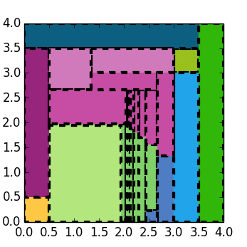
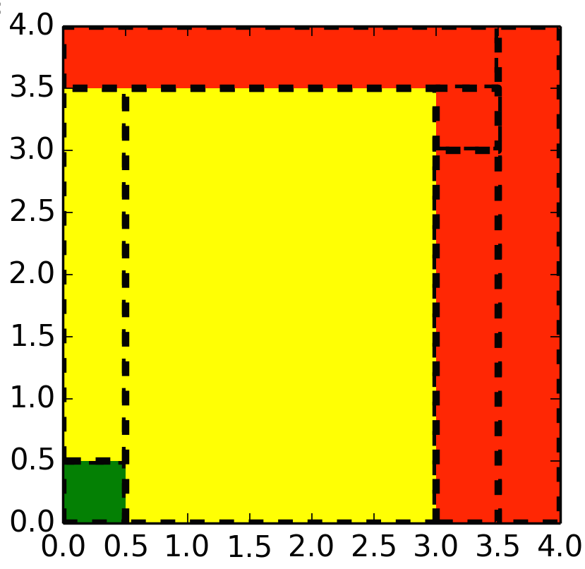
Figure 4: (a) shows the partition by TuLiP of the system (14) when the threshold volume was chosen to be 1.0. Regions of the same color are considered as one discrete state. (b) shows the partition resulting from our algorithm, with the winning (green), maybe (yellow) and losing (red) sets marked. Here, every region is its own discrete state.

Figure 4a) shows the partition that TuLiP provided when the threshold volume was set to 1.0. Note that the invariant region is finely partitioned. The runtime of the algorithm was 620 s. No controller that fulfills the specifications could be synthesized using this abstraction. Note that from the output of TuLiP, it is not possible to say whether no winning controller exists, or if a winning controller of the original system exists but TuLiP cannot find it because of the partition being too coarse.

The output of our algorithm can be seen in Figure 4b). The coloring illustrates the winning (green), maybe (yellow) and losing (red) states. The states in the maybe set are marked as such since some of the continuous states in them lie within the invariant region, and some lie within the region that can reach goal. Since start lies in the losing set, the algorithm terminates and concludes with a definitive answer that there exists no winning controller (neither for the abstraction nor the original system). This took 25 s.

VI Conclusion

In this paper we have presented an iterative method for abstracting a discrete-time control system into two FTSs, representing an under- and over-approximation of the reachability properties of the original dynamical system. We have provided theorems regarding the existence of controllers fulfilling GR1-specifications for the continuous system, based on the existence of such controllers for the two FTSs. Our proposed algorithm provides a way of focusing the computational resources on refining only certain areas of the state space, leading to a decrease in the time complexity of the abstraction procedure compared to previous methods. We have made a comparison between the proposed algorithm and the one currently used in the TuLiP-framework on numerical examples with promising results.

Proof of Proposition 1.

Let us define an index function $h:\bigcup_{i\in\mathcal{I}}\mathcal{W}_{i}\rightarrow\mathcal{I}$, such that for any $\varsigma\in\bigcup_{i\in\mathcal{I}}\mathcal{W}_{i}$, the following set inclusion holds:

$$\varsigma\in\mathcal{W}_{h(\varsigma)}.$$

Now assume that the winning controller for the set $\mathcal{W}_{i}$ is $\gamma^{(i)}=(\gamma_{1}^{(i)},\gamma_{2}^{(i)},\dots,\gamma_{t}^{(i)},\dots)$. We can define the new controller $\gamma=(\gamma_{1},\gamma_{2},\dots)$ as

$$\gamma_{t}(\varsigma[0],e[0],\dots,e[t-1])=\gamma_{t}^{(h(\varsigma[0]))}(\varsigma[0],e[0],\dots,e[t-1]).$$

It is easily verified that $\gamma$ is a winning controller for
$\bigcup_{i\in\mathcal{I}}\mathcal{W}_{i}$. ∎

Lemma 1.

For any two sequences $\sigma=\nu_{0}\nu_{1}\dots$, $\sigma^{\prime}=\nu_{0}^{\prime}\nu_{1}^{\prime}\dots$, such that $\sigma\models\varphi$ and $\sigma^{\prime}\models\varphi$, where $\varphi$ is a GR1 formula defined in (1), the following properties hold:

1. Define a time-shifted sequence $\sigma_{t}=\nu_{t}\nu_{t+1}\dots$, then $\sigma_{t}\models\varphi$.

2. Suppose that there exists $\tau\geq 0$, such that $\nu_{\tau}=\nu^{\prime}_{0}$, then the following sequence $\nu_{0}\dots\nu_{\tau}\nu^{\prime}_{1}\nu^{\prime}_{2}\dots\models\varphi$.

Proof.

By definition, $\sigma\models\varphi$ if and only if

$$\sigma\models\left(\neg\bigwedge_{i=1}^{M}\square\lozenge p_{i}\right)\bigvee\left(\bigwedge_{j=1}^{N}\square\lozenge q_{j}\right).$$ (15)

The lemma follows directly from the fact that the right hand side of (15) is a liveness formula. ∎

Lemma 2.

Consider an FTS $\mathbb{T}$ and a GR1 formula $\varphi$. If the controller $\gamma$ is winning for some non-empty set $\mathcal{W}$, then for any initial condition $\varsigma[0]\in\mathcal{W}$ and environmental actions $e[0]e[1]\dots$, the controlled execution $(\varsigma[0],e[0])(\varsigma[1],e[1])\dots$ satisfies

$$\varsigma[t]\in W(\mathbb{T},\varphi),\,\forall t=0,1,\dots\;.$$

Proof.

This result follows directly from Lemma 1. ∎

Proof of Theorem 10.

By the recursive definition of $\mathbb{D}^{(i)}_{p}$ and $\mathbb{D}^{(i)}_{o}$, we know that for any $\varsigma_{a},\varsigma_{b}\in\mathcal{S}^{(i)}$,

$$(\varsigma_{a},e_{a})\rightarrow_{p}^{(i)}(\varsigma_{b},e_{b})$$

implies that

$$\mathcal{R}_{p}(T^{-1}_{\mathcal{S}^{(i)}}(\varsigma_{a})),T^{-1}_{\mathcal{S}^{(i)}}(\varsigma_{b})))=1.$$

Hence, (9) can be proved in a similar way as Theorem 1.

We now prove (10). For the FTS $\mathbb{D}_{p}^{(i)}$, suppose the winning controller for $\mathcal{W}^{(i)}=W(\mathbb{D}^{(i)}_{p},\varphi)$ is $\gamma_{p}^{(i)}=(\gamma_{p,1}^{(i)},\gamma_{p,2}^{(i)},\dots)$. We can define the controller $\gamma_{p}^{(i+1)}=(\gamma_{p,1}^{(i+1)},\gamma_{p,2}^{(i+1)},$ $\dots)$ for the FTS $\mathbb{D}_{p}^{(i+1)}$ as

$$\gamma_{p,t}^{(i+1)}((\varsigma[0],1), e[0],\dots,e[t-1])$$

$$=(\gamma_{p,t}^{(i)}(\varsigma[0],e[0],\dots,e[t-1]),1).$$

Thus, the controlled execution of the FTS $\mathbb{D}_{p}^{(i+1)}$ is given by

$$((\varsigma[0],1),e[0])((\varsigma[1],1),e[1])((\varsigma[2],1),e[2])\dots,$$

which satisfies the specification $\varphi$. Therefore, we only need to prove that the controller $\gamma_{p}^{(i+1)}$ is consistent.

By Lemma 2, we know that for any $\varsigma[0]\in\mathcal{W}^{(i)}$, the controlled execution $(\varsigma[0],e[0])\dots$ satisfies

$$\varsigma[t]\in\mathcal{W}^{(i)},$$

which implies that the transition from $((\varsigma[t],1),e[t])$ to $((\varsigma[t+1],1),e[t+1])$ in $\mathbb{D}_{p}^{(i+1)}$ is a WW-transition and hence exists. Hence, $\gamma_{p}^{(i+1)}$ is consistent, which completes the proof. ∎

Proof of Theorem 4.

We first prove (12). Notice that by the construction of $\mathbb{D}_{o}^{(i+1)}$, if $\varsigma[0]\in\mathcal{L}^{(i)}=L(\mathbb{D}_{o}^{(i)},\varphi)$, then $((\varsigma[0],1),e[0])$ has no successors in $\mathbb{D}_{o}^{(i+1)}$. Thus, $(\varsigma[0],1)\in L(\mathbb{D}_{o}^{(i+1)},\varphi)$ since no consistent controller exists for $(\varsigma[0],1)$.

We now prove (11) by induction. Notice that we cannot use the same argument as Theorem 2 since $s_{a}\rightarrow s_{b}$ does not necessarily imply $T_{\mathcal{S}^{(i+1)}}(s_{a})\rightarrow_{o}^{(i+1)}T_{\mathcal{S}^{(i+1)}}(s_{b})$.

By Theorem 2, we know that (11) holds when $i=1$. For the transition system $TS(\Sigma)$, suppose that the controller $\gamma=(\gamma_{1},\gamma_{2},\dots)$ is winning for $W(TS(\Sigma),\varphi)$. For any $s[0]\in W(TS(\Sigma),\varphi)$ and environmental actions $e[0]e[1]\dots$, we create a controlled execution using $\gamma$: $\sigma=(s[0],e[0])(s[1],e[1])\dots$, which is winning.

Let us define a hitting time $\tau$ as

$$\tau=\inf\{t\in\mathbb{N}_{0}:T_{\mathcal{S}^{(i-1)}}(s[t])\in\mathcal{W}^{(i-1)}\}.$$

In other words, $\tau$ is the first time that $T_{\mathcal{S}^{(i-1)}}(s[t])$ enters the winning set $\mathcal{W}^{(i-1)}$. We further assume that the infimum over an empty set is $\infty$.

For the FTS $\mathbb{D}_{p}^{(i-1)}$, suppose that the controller $\gamma_{p}=(\gamma_{p,1},\dots)$ is winning for $W(\mathbb{D}_{p}^{(i-1)},\varphi)=\mathcal{W}^{(i-1)}$. If $\tau<\infty$, we define $\varsigma_{p}[0]=T_{\mathcal{S}^{(i-1)}}(s[\tau])$ and $e_{p}[t]=e[t+\tau]$. Now we create a controlled execution using $\gamma_{p}$ with environmental actions $e_{p}[0]e_{p}[+1]\dots$: $\sigma_{p}=(\varsigma_{p}[0],e_{p}[0])(\varsigma_{p}[1],e_{p}[1])\dots$, which is also winning.

We now construct a controller $\gamma_{o}=(\gamma_{o,1},\dots)$ of the FTS $\mathbb{D}_{o}^{(i)}$, such that it is winning at $\varsigma[0]=T_{\mathcal{S}^{(i)}}(s[0])$. The construction can by divided into two steps:

1. If $t\leq\tau$, then $\gamma_{o}$ follows the winning controller $\gamma$ of the FTS $TS(\Sigma)$, i.e.,

   $$\gamma_{o,t}(\varsigma[0], e[0],\dots,e[t-1])$$

   $$=T_{\mathcal{S}^{(i)}}(\gamma_{t}(s[0],e[0],\dots,e[t-1])).$$

2. If $t>\tau$, we switch to the winning controller $\gamma_{p}$ of the FTS $\mathbb{D}_{p}^{(i-1)}$, i.e.,

   $$\gamma_{o,t} (\varsigma[0],e[0],\dots,e[t-1])$$

   $$=(\gamma_{p,t-\tau}(\varsigma_{p}[0],e_{p}[0],\dots,e_{p}[t-\tau-1]),1).$$

Now we prove that $\gamma_{o}$ is winning at $\varsigma[0]$. Define the controlled execution using $\gamma_{o}$ on the FTS $\mathbb{D}_{o}^{(i)}$ to be

$$\sigma_{o}=(\varsigma_{o}[0],e[0])(\varsigma_{o}[1],e[1])\dots\;.$$

We need to prove that $\sigma_{o}$ satisfies the specification and $\gamma_{o}$ is consistent. The proof is divided into two cases depending on whether $\tau=\infty$ or $\tau<\infty$.

Case 1: $\tau=\infty$

By the definition of $\gamma_{o}$, we know that

$$\varsigma_{o}[t]=T_{\mathcal{S}^{(i)}}(s[t]).$$

Since $\sigma$ is winning, we only need to check the consistency of $\gamma_{o}$, i.e., whether the transition from $(\varsigma_{o}[t],e[t])$ to $(\varsigma_{o}[t+1],e[t+1])$ exists in $\mathbb{D}_{o}^{(i)}$. By Lemma 2, we know that

$$s[t]\in W(TS(\Sigma),\varphi).$$

And hence, by the induction assumption,

$$T_{\mathcal{S}^{(i-1)}}(s[t])\in\mathcal{M}^{(i-1)}\bigcup\mathcal{W}^{(i-1)}.$$

By the fact that $\tau=\infty$,

$$T_{\mathcal{S}^{(i-1)}}(s[t])\in\mathcal{M}^{(i-1)}.$$

As a result, there exists an $j_{t}\in\{1,\dots,m\}$, such that $\varsigma_{o}[t]$ is the $j_{t}$th child of $T_{\mathcal{S}^{(i-1)}}(s[t])$, i.e.,

$$\varsigma_{o}[t]=(T_{\mathcal{S}^{(i-1)}}(s[t]),j_{t}).$$

Furthermore, since there exists an $u[t]$, such that $f(s[t],u[t])=s[t+1]$, we know that

$$\mathcal{R}_{o}(T^{-1}_{\mathcal{S}^{(i)}}(\varsigma_{o}[t]),T^{-1}_{\mathcal{S}^{(i)}}(\varsigma_{o}[t+1]))=1,$$

Hence, the transition from $(\varsigma_{o}[t],e[t])$ to $(\varsigma_{o}[t+1],e[t+1])$ is an MM-transition and it exists in $\mathbb{D}_{o}^{(i)}$. And thus, $\gamma_{o}$ is consistent.

Case 2: $\tau<\infty$

By the construction of $\gamma_{o}$, $\sigma_{o}$ satisfies

$$\varsigma_{o}[t]=\begin{cases}T_{\mathcal{S}^{(i)}}(s[t])&\text{if }t\leq\tau,\\ (\varsigma_{p}[t-\tau],1)&\text{if }t>\tau.\\ \end{cases}$$

By Lemma 1 and the fact that both $\sigma$ and $\sigma_{p}$ satisfy $\varphi$, we only need to check the consistency of $\gamma_{o}$, i.e., whether the transition from $(\varsigma_{o}[t],e[t])$ to $(\varsigma_{o}[t+1],e[t+1])$ exists in $\mathbb{D}_{o}^{(i)}$. This can be done in three steps:

1. $t<\tau-1$:

   By the same argument as for the case where $\tau=\infty$, we know that the transition from $(\varsigma_{o}[t],e[t])$ to $(\varsigma_{o}[t+1],e[t+1])$ is an MM-transition and it exists in $\mathbb{D}_{o}^{(i)}$.

2. $t=\tau-1$:

   By the definition of $\tau$, we know that

   $$T_{\mathcal{S}^{(i-1)}}(s[\tau-1])\in\mathcal{M}^{(i-1)},\,T_{\mathcal{S}^{(i-1)}}(s[\tau])\in\mathcal{W}^{(i-1)}.$$

   Hence, the transition from $(\varsigma_{o}[\tau-1],e[\tau-1])$ to $(\varsigma_{o}[\tau],e[\tau])$ is an MW-transition and it exists in $\mathbb{D}_{o}^{(i)}$.

3. $t>\tau-1$:

   By Lemma 2, we know that

   $$\varsigma_{p}[t]\in W(\mathbb{D}_{p}^{(i-1)},\varphi)=\mathcal{W}^{(i-1)}.$$

   Hence, the transition from $(\varsigma_{o}[t],e[t])$ to $(\varsigma_{o}[t+1],e[t+1])$ is a WW-transition and it exists in $\mathbb{D}_{o}^{(i)}$.

Therefore, $\gamma_{o}$ is consistent and we can conclude the proof. ∎

References

- [1] C. Baier and J.-P. Katoen. Principles of Model Checking. MIT Press, 2007.
- [2] A. Bhatia, L. E. Kavraki, and M. Y. Vardi. Sampling-based motion planning with temporal goals. In ICRA, pages 2689–2696, 2010.
- [3] L. De Alfaro and P. Roy. Solving games via three-valued abstraction refinement. In CONCUR 2007 - Concurrency Theory, pages 74–89. Springer, 2007.
- [4] G. E. Fainekos, A. Girard, H. Kress-Gazit, and G. J. Pappas. Temporal logic motion planning for dynamic robots. Automatica, 45(2):343 – 352, 2009.
- [5] S. Karaman and E. Frazzoli. Sampling-based motion planning with deterministic -calculus specifications. In CDC, 2009.
- [6] M. Kloetzer. and C. Belta. Automatic deployment of distributed teams of robots from temporal logic motion specifications. IEEE Transactions on Robotics, 26(1):48–61, 2010.
- [7] H. Kress-Gazit, G. E. Fainekos, and G. J. Pappas. Temporal-logic-based reactive mission and motion planning. IEEE Transactions on Robotics, 25(6):1370–1381, 2009.
- [8] T. Moor, J. Davoren, and J. Raisch. Learning by doing: systematic abstraction refinement for hybrid control synthesis. IEE Proceedings - Control Theory and Applications, 153(5):591–599, Sept. 2006.
- [9] P. Nuzzo, H. Xu, N. Ozay, J. Finn, A. Sangiovanni-Vincentelli, R. Murray, A. Donze, and S. Seshia. A contract-based methodology for aircraft electric power system design. Access, IEEE, PP(99):1–1, 2013.
- [10] N. Piterman, A. Pnueli, and Y. Sa’ar. Synthesis of reactive (1) designs. In Verification, Model Checking, and Abstract Interpretation, pages 364–380. Springer, 2006.
- [11] A. Pnueli and R. Rosner. On the synthesis of a reactive module. In Proceedings of the 16th ACM SIGPLAN-SIGACT Symposium on Principles of Programming Languages, POPL ’89, pages 179–190, New York, NY, USA, 1989. ACM.
- [12] S. V. Rakovic, E. Kerrigan, D. Mayne, and J. Lygeros. Reachability analysis of discrete-time systems with disturbances. IEEE Transactions on Automatic Control, 51:546–561, Apr. 2006.
- [13] V. Raman, M. Maasoumy, A. Donzé, R. M. Murray, A. Sangiovanni-Vincentelli, and S. Seshia. Model predictive control with signal temporal logic specifications. In IEEE Conference on Decision and Control (CDC), 2014.
- [14] P. Tabuada. An approximate simulation approach to symbolic control. IEEE Trans. Automat. Contr., 53(6):1406–1418, 2008.
- [15] P. Tabuada. Verification and Control of Hybrid Systems: A Symbolic Approach. Springer Publishing Company, Incorporated, 1st edition, 2009.
- [16] R. Vidal, S. Schaffert, J. Lygeros, and S. Sastry. Controlled Invariance of Discrete Time Systems. Lecture Notes in Computer Science LNCS, (1790):437–450, 2000.
- [17] T. Wongpiromsarn, U. Topcu, and R. Murray. Receding horizon temporal logic planning for dynamical systems. Proc. IEEE Conf. Decision Control, pages 5997–6004, 2009.
- [18] T. Wongpiromsarn, U. Topcu, and R. Murray. Receding horizon temporal logic planning. Automatic Control, IEEE Transactions on, 11(57):2817–2830, 2012.
- [19] T. Wongpiromsarn, U. Topcu, and R. M. Murray. Synthesis of control protocols for autonomous systems. Unmanned Systems, 01(01):21–39, 2013.
- [20] T. Wongpiromsarn, U. Topcu, N. Ozay, H. Xu, and R. M. Murray. Tulip: a software toolbox for receding horizon temporal logic planning. In HSCC, pages 313–314, 2011.
- [21] M. Zamani, G. Pola, M. Mazo, and P. Tabuada. Symbolic models for nonlinear control systems without stability assumptions. Automatic Control, IEEE Transactions on, 57(7):1804–1809, 2012.