Two-particle correlations in pseudorapidity in a hydrodynamic model

Abstract

Two-particle pseudorapidity correlations of hadrons produced in Pb+Pb collisions at $\sqrt{s_{NN}}=2.76$ TeV at the CERN Large Hadron Collider are analyzed in the framework of a model based on viscous 3+1-dimensional hydrodynamics with the Glauber initial condition. Based on our results, we argue that the correlation from resonance decays, formed at a late stage of the evolution, produce significant effects. In particular, their contribution to the event averages of the coefficients of the expansion in the Legendre basis explain 60-70% of the experimental values. We have proposed an accurate way to compute these coefficients, independent of the binning in pseudorapidity, and tested a double expansion of the two-particle correlation function in the azimuth and pseudorapidity, which allows us to investigate the pseudorapidity correlations between harmonics of the collective flow. In our model, these quantities are also dominated by non-flow effects from the resonance decays. Finally, our method can be used to compute higher-order cumulants for the expansion in orthonormal polynomials Bzdak:2015dja which offers a suitable way of eliminating the non-flow effects from the correlation analyses.

I Introduction

The mechanism of energy deposition in relativistic nuclear collisions is a subject of intense studies. Whereas most of the investigations are concerned with the entropy-deposition profile in the transverse plane and the resulting transverse expansion (for reviews see, e.g., Heinz:2013th ; Gale:2013da ), the dynamics in the longitudinal direction is less explored, and has been recently gaining more attention with the new experimental analyses from the CERN Large Hadron Collider (LHC) expected shortly. Such studies could give valuable insight into the initial energy and momentum distributions in rapidity Dusling:2009ni ; *Armesto:2006bv; *Fukushima:2008ya, the longitudinal collective dynamics Bozek:2007qt ; *Ryblewski:2012rr; *Martinez:2010sc; *Casalderrey-Solana:2013sxa, or hydrodynamic fluctuations Kapusta:2011gt ; *Gavin:2011gr. Correlations in (pseudo)rapidity can be studied in various ways, in particular, as correlations of the transverse flow at different rapidity bins, or as multiplicity correlations in rapidity. The first case requires an intermediate collective expansion stage producing flow Bozek:2010vz ; Petersen:2011fp ; *Xiao:2012uw; *Jia:2014ysa; *Jia:2014vja; *Pang:2014pxa; *Khachatryan:2015oea; Bozek:2015bna ; Bozek:2015bha , whereas the particle distribution and multiplicity correlations in rapidity are not modified significantly during the fireball expansion, thus are expected to reflect more closely the initial conditions in the fireball. In other words, the multiplicity correlations arise even without any collective expansion.

Correlations of the multiplicity of particles observed in high energy collisions in different pseudorapidity intervals have been studied in a number of colliding systems Bzdak:2012tp ; Dusling:2009ni ; Back:2006id ; *Bzdak:2009xq; *Abelev:2009ag; *Feofilov:2013kna; *De:2013bta; *Amelin:1994mf; *Braun:1997ch; *Brogueira:2006yk; *Yan:2010et; *Bialas:2011xk; *Olszewski:2013qwa; *Olszewski:2015xba. The most common approach is based on the correlation of the number of particles in forward and a backward pseudorapidity bins, $\langle n_{F}n_{B}\rangle$, or related observables.

Bzdak and Teaney have proposed to expand the two-point correlation function in pseudorapidity in a basis of orthogonal polynomials Bzdak:2012tp . The correlations are then written in terms of the corresponding expansion coefficients $\langle a_{n}a_{m}\rangle$. The extracted coefficients can serve to parametrize event by event fluctuations of the particle distribution in pseudorapidity. A basis of the Legendre polynomials Jia:2015jga has been used for the expansion of the correlation in pseudorapidity for the case of Pb+Pb collisions at $\sqrt{s}=2760$ GeV, recently measured by the ATLAS Collaboration ATLAS:2015kla ; *AnmTALK.

In this work we present predictions of the relativistic hydrodynamic model for the two-particle correlations in pseudorapidity, focusing on correlations generated in the late stage of the collision via resonance decays. Our approach consists of a Glauber Monte Carlo model with asymmetric longitudinal emission profile for the initial state, and the viscous 3+1D hydrodynamic evolution of the fireball, followed by statistical hadron emission at freeze-out. Our main result is that the late-stage correlations from resonance decays contribute largely (about a half of the measured values) to the correlations extracted in terms of the $\langle a_{n}a_{m}\rangle$ coefficients. The missing strength should be attributed to the correlations generated in the earlier stages of the evolution (initial state, jets).

II Two-particle correlation

The two-particle correlation in pseudorapidity, scaled by the one-particle distributions, is defined as

$$C(\eta_{1},\eta_{2})=\frac{\langle N(\eta_{1})N(\eta_{2})\rangle-\langle N(\eta_{1})\rangle\delta(\eta_{1}-\eta_{2})}{\langle N(\eta_{1})\rangle\langle N(\eta_{2})\rangle}\ ,$$ (1)

where $N(\eta)$ denotes the distribution of the number of hadrons at $\eta$ and the averaging is over events in a selected centrality class. In the experiment, the correlation function is constructed as the ratio of the histogram for particle pairs from physical events to the histogram constructed from mixed events in the same centrality class ATLAS:2015kla

$$C(\eta_{1},\eta_{2})=\frac{S(\eta_{1},\eta_{2})}{B(\eta_{1},\eta_{2})}\ .$$ (2)

We note that the definition  (1) corresponds to the scaled second factorial moment of the multiplicity distribution, which depends on the centrality definition and the width of the centrality bin. To reduce the effects of the overall multiplicity fluctuations, the ATLAS collaboration uses a modified correlation function

$$C_{N}(\eta_{1},\eta_{2})=\frac{C(\eta_{1},\eta_{2})}{C_{p}(\eta_{1})C_{p}(\eta_{2})}\ ,$$ (3)

with $C_{p}(\eta_{1})=\frac{1}{2Y}\int_{-Y}^{Y}C(\eta_{1},\eta_{2})d\eta_{2}$. The experimental analysis suggests that $C_{N}(\eta_{1},\eta_{2})$ is approximately independent of the definition of centrality Jia:2015jga ; ATLAS:2015kla .

III Expansion in orthonormal polynomials

As the shape of the distribution function ${N(\eta)}/{\langle N(\eta)\rangle}$ fluctuates event by event, it can be expanded in a basis of orthogonal functions Bzdak:2012tp

$$\frac{N(\eta)}{\langle N(\eta)\rangle}=1+\sum_{n=0}^{\infty}a_{n}T_{n}\left(\frac{\eta}{Y}\right)\ .$$ (4)

For the case of Legendre polynomials $P_{n}(x)$, the normalized functions are $T_{n}(\frac{\eta}{Y})=\sqrt{\frac{2n+1}{2}}P_{n}(x)$ Jia:2015jga , where $[-Y,Y]$ is the pseudorapidity range on which the correlation functions are measured, such that the orthonormality condition takes the form

$$\int_{-Y}^{Y}T_{n}\left(\frac{\eta}{Y}\right)T_{m}\left(\frac{\eta}{Y}\right)\frac{d\eta}{Y}=\delta_{nm}\ .$$ (5)

The event-average $\langle a_{n}a_{m}\rangle$ can be calculated from the two-particle correlation function

$$\langle a_{n}a_{m}\rangle=\int_{-Y}^{Y}\frac{d\eta_{1}}{Y}\int_{-Y}^{Y}\frac{d\eta_{2}}{Y}C(\eta_{1},\eta_{2})T_{n}\left(\frac{\eta_{1}}{Y}\right)T_{m}\left(\frac{\eta_{1}}{Y}\right)\ .$$ (6)

The procedure is rather complicated, as first the two-particle correlation function must be constructed with sufficiently fine binning. In the case of low statistics, large binning of $C$ introduces biases.

The estimate of the integral (6) can be simply obtained from

$$\langle a_{n}a_{m}\rangle = \left\langle\sum_{a\neq b}\frac{T_{n}\left(\frac{\eta_{a}}{Y}\right)}{Y\langle N(\eta_{a})\rangle}\frac{T_{m}\left(\frac{\eta_{b}}{Y}\right)}{Y\langle N(\eta_{b})\rangle}\right\rangle$$

$$= \left\langle{\sum_{a}\frac{T_{n}\left(\frac{\eta_{a}}{Y}\right)}{Y\langle N(\eta_{a})\rangle}\sum_{b}\frac{T_{m}\left(\frac{\eta_{b}}{Y}\right)}{Y\langle N(\eta_{b})\rangle}}\right\rangle$$

$$- \left\langle\sum_{a}\frac{T_{n}\left(\frac{\eta_{a}}{Y}\right)}{Y\langle N(\eta_{a})\rangle}\frac{T_{m}\left(\frac{\eta_{a}}{Y}\right)}{Y\langle N(\eta_{a})\rangle}\right\rangle\ ,$$

where the sums are over hadrons in the given event and the averages are over events. Equation (III) produces very stable results, free of the binning bias.

In the experimental analysis of Ref. ATLAS:2015kla the function $C_{N}(\eta_{1},\eta_{2})$ instead of $C(\eta_{1},\eta_{2})$ is used in Eq. (6). We have checked that in our case the resulting difference for the $\langle a_{n}a_{m}\rangle$ coefficients for $1\leq n,m\leq 5$ is very small, a fraction of percent, hence in the following we will use $C(\eta_{1},\eta_{2})$ in Eq. (III). In addition, the function $C(\eta_{1},\eta_{2})$ is, in the experiment, normalized to 1. To conform to this convention we rescale the coefficients obtained from Eq. (III):

$$\langle a_{n}a_{m}\rangle\to\frac{\langle a_{n}a_{m}\rangle}{1+\langle a_{0}a_{0}\rangle/2}\ .$$ (8)

In practice, for centrality bins in the model calculation defined by the number of participant nucleons, the correction to the normalization is less than 2%.

The motivation of the studies of Ref. Bzdak:2012tp ; Jia:2015jga ; ATLAS:2015kla was to transform the two-particle distributions into a series of coefficients $\langle a_{n}a_{m}\rangle$ with a simple interpretation. For instance, the coefficient $\langle a_{1}a_{1}\rangle$ is related to the asymmetry in the entropy deposition in rapidity from the forward and backward going participant nucleons. The asymmetry of the deposition in rapidity is visible in the charged particle distribution in pseudorapidity in asymmetric collisions Bialas:2004su and in forward-backward multiplicity distributions Bzdak:2009xq .

IV Results from the hydrodynamic model

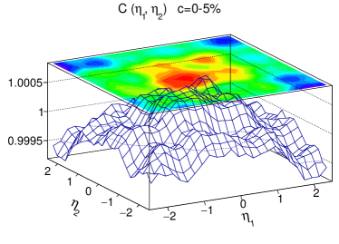
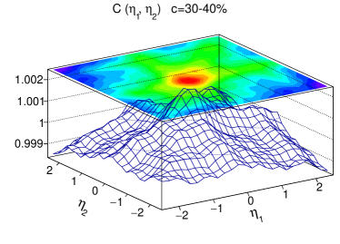
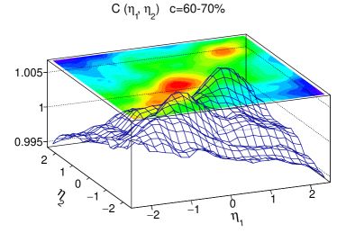
Figure 1: (color online) Two dimensional correlation function in pseudorapidity for charged particles in Pb+Pb collisions at $\sqrt{s}=2.76$ TeV at three centrality classes 0-5%, 30-40% and 60-70% in panels (a), (b) and (c), respectively.

We use the 3+1-dimensional viscous hydrodynamics Bozek:2011ua to model the evolution of the fireball created in Pb+Pb collisions at $\sqrt{s}=2.76$ TeV. The initial entropy density in the transverse plane is calculated in GLISSANDO Broniowski:2007nz ; *Rybczynski:2013yba, implementing the Glauber Monte Carlo model. The initial profile in the longitudinal direction (in space-time rapidity) is considered in two qualitatively different scenarios. In the first scenario, the entropy distribution in space-time rapidity from a left- and right-going participant nucleons is of the form

$$f_{\pm}(\eta_{\parallel})=\frac{\eta_{\rm beam}\pm\eta_{\parallel}}{y_{\rm beam}}H(\eta_{\parallel})\ \mbox{\rm for }\ |\eta_{\parallel}|<y_{\rm beam}\ ,$$ (9)

where

$$H(\eta_{\parallel})=\exp\left(-\frac{(|\eta_{\parallel}|-\eta_{p})^{2}\Theta(|\eta_{\parallel}|-\eta_{p})}{2\sigma_{\eta}^{2}}\right),$$ (10)

and $y_{\rm beam}$ is the rapidity of the beam. For the LHC, the parameters determining the shape are $\sigma=1.4$ and $\eta_{p}=2.4$. The asymmetric distribution of the deposited entropy between the forward and backward rapidity hemisphere leads, together with the fluctuations in the number of participants, lead to nontrivial correlations between forward and backward rapidity bins, both in multiplicity Bzdak:2009xq and in the flow angle orientation Bozek:2010vz ; *Bozek:2015bha. The latter has been termed the torque effect, hence we label our calculations based on Eq. (11) as torque.

The reference scenario assumes that the initial entropy profile in space-time rapidity is symmetric,

$$f_{\pm}(\eta_{\parallel})=H(\eta_{\parallel})\ \mbox{for }\ |\eta_{\parallel}|<y_{\rm beam}\ .$$ (11)

In that case (labeled no torque) in each event the fireball density has a backward-forward symmetry, hence no shape fluctuations of odd reflection symmetry are possible. To summarize, the torque case includes certain initial-state fluctuations in rapidity, while the no-torque case does not.

At freeze-out, hadrons are emitted, and later resonance decays occur. The decays of resonances introduce short-range correlations of length of about one unit in pseudorapidity, leading to a nontrivial structure of the two-dimensional correlation functions. Note that another source of correlation in the late stage, unrelated to the fireball shape fluctuations, is due to local charge conservation Jeon:2001ue ; Bozek:2012en .

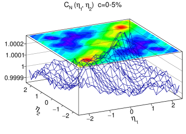
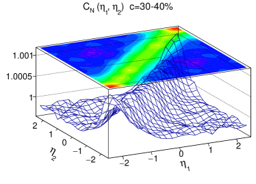
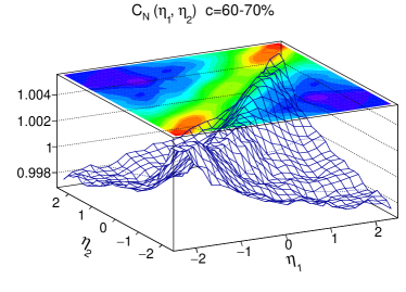
Figure 2: (color online) Same as Fig. 1 but for the corrected correlations function $C_{N}(\eta_{1},\eta_{2})$ (3).

The correlation function (2) is calculated from realistic, finite-multiplicity events, generated after the hydrodynamic evolution with THERMINATOR Kisiel:2005hn ; *Chojnacki:2011hb. We use the freeze-out temperature $T_{f}=150$ MeV. The simulated events include the short-range correlations from resonance decays. In Fig. 1 we show the two-dimensional correlations for three different centrality classes. Charged particles with $p_{\perp}>0.5$ GeV and $|\eta|<2.5$ are taken to simulate the ATLAS acceptance.

For $C(\eta_{1},\eta_{2})$, plotted in Fig. 1 for three sample centralities, a peak from the short range correlations is clearly visible around $\eta_{1}\simeq\eta_{2}$. When passing to $C_{N}(\eta_{1},\eta_{2})$, we note that the denominator in Eq. (3) is smaller than one at large $|\eta_{1,2}|$, hence it causes relative enhancement of the correlation measure in this region. As a result, the shape of the correlation function is changed significantly when passing from $C(\eta_{1},\eta_{2})$ to $C_{N}(\eta_{1},\eta_{2})$, cf. Figs. 1 and 2. In particular, a saddle-like form appears, corresponding to a term of the form $A(\eta_{+}^{2}-\eta_{-}^{2})$, where $\eta_{\pm}=\eta_{1}\pm\eta_{2}$. Such a term is expected from event-by-event asymmetry of the initial distribution function Bzdak:2012tp , giving a nonzero value of $\langle a_{1}a_{1}\rangle$. Without this asymmetry, the short-range correlations are expected to be a function of $|\eta_{1}-\eta_{2}|$ only Xu:2012ue ; *Xu:2013sua.

However, in our simulations almost the same value of $\langle a_{1}a_{1}\rangle$ is obtained from the correlation functions $C(\eta_{1},\eta_{2})$ and $C_{N}(\eta_{1},\eta_{2})$. It thus suggests that the observed dependence of the correlation function on $\eta_{\pm}$ does not directly prove the existence of correlations induced by the event-by-event fluctuations of the distribution.

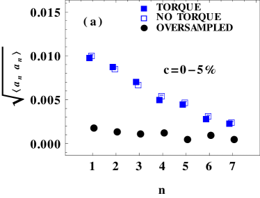
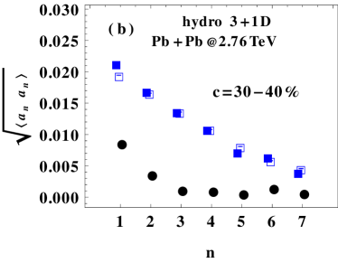
Figure 3: (color online) Calculated coefficients $\sqrt{\langle a_{n}a_{n}\rangle}$ for centrality $0-5$% (panel a) and $30-40$% (panel b) for the torque and no-torque models, as well as for the oversampled events for the torque case (see text for details).

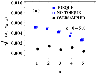
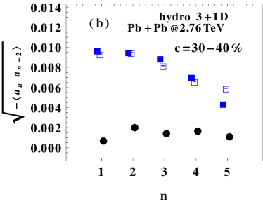
Figure 4: (color online) Same as in Fig. 3 but for the the coefficients $\sqrt{-\langle a_{n}a_{n+2}\rangle}$.

In Fig. 3 we show the calculated coefficients $\sqrt{\langle a_{n}a_{n}\rangle}$, $n=1,\dots,7$ for two sample centralities. The magnitude predicted by the model reaches about 60-70% of the values observed experimentally ATLAS:2015kla . The trend of the dependence on the rank $n$ is similar as in the experiment. Similar conclusions can be made for the non-diagonal coefficients $\sqrt{-\langle a_{n}a_{n+2}\rangle}$ shown in Fig. 4. With the available statistics, we cannot calculate higher order averages $\langle a_{n}a_{n+4}\rangle$. The results for the two scenarios of the the initial conditions, torque and no-torque, are shown. Interestingly, both calculations give very similar results. This shows that in our model the dominant contribution in the observed signal comes from the short-range correlations due to resonance decays.

V Double expansion of correlations functions in azimuthal angle and pseudorapidity

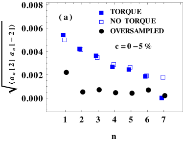
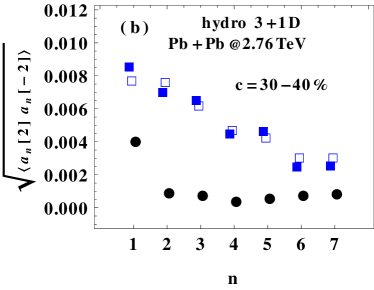
Figure 5: (color online) Same as in Fig. 3 but for the the coefficients of the second order harmonic $\sqrt{\langle a_{n}[2]a_{n}[-2]\rangle}$.

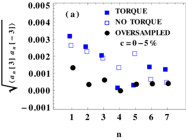
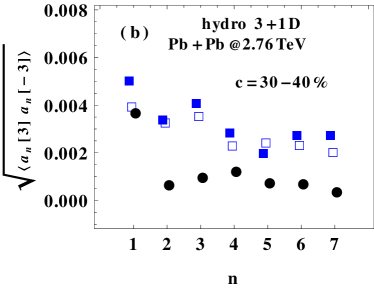
Figure 6: (color online) Same as in Fig. 3 but for the coefficients of the third harmonic $\sqrt{\langle a_{n}[3]a_{n}[-3]\rangle}$.

Collective flow in ultrarelativistic heavy-ion collisions causes all particles to be emitted in a correlated way, which leads to azimuthal asymmetry in hadron distributions. The correlation function between two pseudorapidity bins, constructed for multiplicity correlations as in the preceding sections, can be straightforwardly generalized for each harmonic flow component for any two pseudorapidity bins. Various techniques are applicable here. The rapidity dependence could be decomposed into principal components Bhalerao:2014mua , but in practice the principal component analysis may be difficult and restricted to the lowest eigenmodes. Alternatively, the harmonic flow correlations in pseudorapidity can be expanded in a basis of suitable orthogonal polynomials, in full analogy to the multiplicity case. This provides insight into a different characteristic of the flow, with possibly different sensitivity to non-flow effects than in the multiplicity correlations discussed in Sec. II.

Let us define the correlation coefficients for the $n$-th order harmonic flow as

$$\langle a_{j}[n]a_{k}[-n]\rangle=\left\langle\sum_{a\neq b}\frac{T_{i}\left(\frac{\eta_{a}}{Y}\right)e^{in\phi_{a}}}{Y\langle N(\eta_{a})\rangle}\frac{T_{k}\left(\frac{\eta_{b}}{Y}\right)e^{-in\phi_{b}}}{Y\langle N(\eta_{b})\rangle}\right\rangle\ .$$ (12)

In the above equation, use we the normalization of the correlations function by ${1}/{\langle N(\eta_{1})\rangle\langle N(\eta_{2})\rangle}$ as in Eq. (1), but the formula can be written analogously for the correlation function of flow vectors in two rapidity intervals as used in Bhalerao:2014mua . Note that the linear part of the pseudorapidity dependence of the torque effect for the orientation of the flow angle Bozek:2010vz contributes to the $\langle a_{1}[n]a_{1}[-n]\rangle$ coefficient.

In Figs. 5 and 6 we show the decomposition coefficients (12) of the elliptic and triangular flow correlation at different pseudorapidities. We compare calculations using the torque and no-torque scenarios for the initial conditions, as in Sect. IV. We notice that the two calculation give similar results, although in the no-torque case the odd coefficients should vanish within the statistical uncertainties. Our results mean that in the decomposition of the flow correlations in pseudorapidity, the dominant contribution comes from resonance decays. The same effect has been noticed in the analysis of factorization breaking for flow at different pseudorapidities Bozek:2015bha (the torque effect).

VI Higher-order cumulants

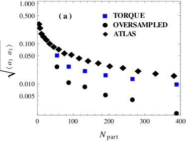
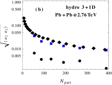
Figure 7: (color online) Coefficients $\sqrt{\langle a_{1}a_{1}\rangle}$ (panel a) and $\sqrt{\langle a_{2}a_{2}\rangle}$ (panel b) for the torque model and for the oversampled events for the torque case, plotted as functions of the number of participants (determining centrality). The ATLAS data come from Ref. ATLAS:2015kla .

Non-flow correlations have a significant contribution to the measured $\langle a_{n}a_{m}\rangle$ coefficients. In this Section we show results of an idealized calculation with the non-flow effects removed. The coefficients are calculated using oversampled events, where for each hydrodynamic evolution several hundreds of THERMINATOR events are generated and combined together. That way non-flow effects are damped. The procedure is equivalent to a Monte Carlo integration of one-particle densities in each event. The results for $\langle a_{1}a_{1}\rangle$ and $\langle a_{2}a_{2}\rangle$ are show in Fig. 7. The genuine effect due to event by event fluctuations of the rapidity distributions is small. The coefficients from the shape fluctuations are much smaller than correlations from resonance decays. The dependence on the rank $n$ of the coefficients $\langle a_{n}a_{n}\rangle$ from oversampled events is presented in Figs. 3 to 6. As expected in the torque scenario, involving forward-backward asymmetry, $\langle a_{1}a_{1}\rangle$ and $\langle a_{1}[n]a_{1}[-n]\rangle$ have the largest magnitude.

Two particle correlations from resonances are removed in higher order cumulants Bzdak:2015dja , while genuine correlations due to initial-state fluctuations of rapidity distributions (4) do contribute. There are many possible combinations of the fourth-order cumulants that can be used for the purpose. In particular, one can define the simplest fourth-order cumulant for the multiplicity fluctuations as Bzdak:2015dja

$$\langle a_{k}^{4}\rangle_{c} = \left\langle{\sum_{a,b,c,d}}^{{}^{\prime}}\frac{T_{k}\left(\frac{\eta_{a}}{Y}\right)}{Y\langle N(\eta_{a})\rangle}\frac{T_{k}\left(\frac{\eta_{b}}{Y}\right)}{Y\langle N(\eta_{b})\rangle}\frac{T_{k}\left(\frac{\eta_{c}}{Y}\right)}{Y\langle N(\eta_{c})\rangle}\frac{T_{k}\left(\frac{\eta_{d}}{Y}\right)}{Y\langle N(\eta_{d})\rangle}\right\rangle-3\left\langle{\sum_{a,b}}^{{}^{\prime}}\frac{T_{k}\left(\frac{\eta_{a}}{Y}\right)}{Y\langle N(\eta_{a})\rangle}\frac{T_{k}\left(\frac{\eta_{b}}{Y}\right)}{Y\langle N(\eta_{b})\rangle}\right\rangle\ ,$$ (13)

where the subscript $c$ stands for the connected part and the prime denotes summation over different particles. For the flow correlations in pseudorapidity, the most general cumulant is of the form

$$\langle a_{i_{1}}[m_{1}]\dots a_{i_{n}}[m_{n}]\rangle_{c}=\left\langle\sum_{a_{1},\dots,a_{n}}\frac{T_{i_{1}}\left(\frac{\eta_{a_{1}}}{Y}\right)e^{im_{1}\phi_{a_{1}}}}{Y\langle N(\eta_{a_{1}})\rangle}\dots\frac{T_{i_{n}}\left(\frac{\eta_{a_{n}}}{Y}\right)e^{im_{n}\phi_{a_{n}}}}{Y\langle N(\eta_{a_{n}})\rangle}\right\rangle_{c}\ ,$$ (14)

with $\sum_{k=1}^{n}m_{k}=0$. The simplest fourth-order cumulants are

$$\langle a_{k}[n]a_{k}[n]a_{k}[-n]a_{k}[-n]\rangle_{c}=$$ (15)

$$~{}~{}\left\langle{\sum_{a,b,c,d}}^{{}^{\prime}}\frac{T_{k}\left(\frac{\eta_{a}}{Y}\right)e^{in\phi_{a}}}{Y\langle N(\eta_{a})\rangle}\frac{T_{k}\left(\frac{\eta_{b}}{Y}\right)e^{in\phi_{b}}}{Y\langle N(\eta_{b})\rangle}\frac{T_{k}\left(\frac{\eta_{c}}{Y}\right)e^{-in\phi_{c}}}{Y\langle N(\eta_{c})\rangle}\frac{T_{k}\left(\frac{\eta_{d}}{Y}\right)e^{-in\phi_{d}}}{Y\langle N(\eta_{d})\rangle}\right\rangle-2\left\langle{\sum_{a,b}}^{{}^{\prime}}\frac{T_{k}\left(\frac{\eta_{a}}{Y}\right)e^{in\phi_{a}}}{Y\langle N(\eta_{a})\rangle}\frac{T_{k}\left(\frac{\eta_{b}}{Y}\right)e^{-in\phi_{b}}}{Y\langle N(\eta_{b})\rangle}\right\rangle\ .$$

We have attempted to compute the fourth-order cumulants (13) and (15) in our simulation, however, with the available statistics (20000 events in each centrality class) the statistical errors are too large, of the same order as the square of the second order cumulant. The application of the cumulant method Bzdak:2015dja is possible on large-statistics experimental data and the results could be compared to model calculations using one-particle densities (such as the results for the oversampled events presented above) that neglect the non-flow effects.

VII Conclusions

We have checked the predictions of a realistic simulation based on viscous 3+1-dimensional hydrodynamics for the two-particle correlations in pseudorapidity, as measured by the ATLAS collaboration ATLAS:2015kla and found that the correlation from the resonance decays, formed at a late stage of the evolution, produce significant effects. In particular, their contribution to the coefficients $\langle a_{n}a_{m}\rangle$ in the expansion of the correlation function in the Legendre basis take 60-70% of the experimental values.

While our model incorporates only some possible sources of correlations (those from the torque effect and the resonance decays), it shows their relevance in the analyses. Other, not incorporated non-flow effects, include the hadron production from jets, local current conservation, or additional sources of rapidity fluctuations in the initial state Bozek:2015bna .

On the methodological level, we have proposed a new way to compute the $\langle a_{n}a_{m}\rangle$ coefficients, independent of the binning in pseudorapidity, and applied it in our simulations. Also, we have developed a double expansion of the correlation function in the azimuth and pseudorapidity, which allows to probe and quantify the rapidity correlations between harmonics of the collective flow. We have found that in our model these quantities are also dominated by non-flow effects. Our method can be used for higher-order averages of the orthogonal polynomials, in particular for cumulants. This offers a way of eliminating the non-flow effects Bzdak:2015dja , but requires very large statistics, which, fortunately, is available in the experiments. These measures could be compared to model calculations with oversampled events, where sufficient statistics can be achieved.

We note that a study using similar methods and leading to similar results has been independently and simultaneously presented in Ref. Monnai:2015sca .

- (1) A. Bzdak and P. Bożek(2015), arXiv:1509.02967 [hep-ph]
- (2) U. Heinz and R. Snellings, Ann.Rev.Nucl.Part.Sci. 63, 123 (2013)
- (3) C. Gale, S. Jeon, and B. Schenke, Int.J.Mod.Phys. A28, 1340011 (2013)
- (4) K. Dusling, F. Gelis, T. Lappi, and R. Venugopalan, Nucl. Phys. A836, 159 (2010)
- (5) N. Armesto, L. McLerran, and C. Pajares, Nucl. Phys. A781, 201 (2007)
- (6) K. Fukushima and Y. Hidaka, Nucl.Phys. A813, 171 (2008)
- (7) P. Bożek, Phys. Rev. C77, 034911 (2008)
- (8) R. Ryblewski and W. Florkowski, Phys. Rev. C85, 064901 (2012)
- (9) M. Martinez and M. Strickland, Nucl. Phys. A848, 183 (2010)
- (10) J. Casalderrey-Solana, M. P. Heller, D. Mateos, and W. van der Schee, Phys. Rev. Lett. 112, 221602 (2014)
- (11) J. I. Kapusta, B. Muller, and M. Stephanov, Phys. Rev. C85, 054906 (2012)
- (12) S. Gavin and G. Moschelli, Phys. Rev. C85, 014905 (2012)
- (13) P. Bożek, W. Broniowski, and J. Moreira, Phys. Rev. C83, 034911 (2011)
- (14) H. Petersen, V. Bhattacharya, S. A. Bass, and C. Greiner, Phys.Rev. C84, 054908 (2011)
- (15) K. Xiao, F. Liu, and F. Wang, Phys.Rev. C87, 011901 (2013)
- (16) J. Jia and P. Huo, Phys.Rev. C90, 034915 (2014)
- (17) J. Jia and P. Huo, Phys.Rev. C90, 034905 (2014)
- (18) L.-G. Pang, G.-Y. Qin, V. Roy, X.-N. Wang, and G.-L. Ma, Phys. Rev. C91, 044904 (2015)
- (19) V. Khachatryan et al. (CMS)(2015), arXiv:1503.01692 [nucl-ex]
- (20) P. Bożek and W. Broniowski(2015), arXiv:1506.02817 [nucl-th]
- (21) P. Bożek, W. Broniowski, and A. Olszewski, Phys.Rev. C91, 054912 (2015)
- (22) A. Bzdak and D. Teaney, Phys.Rev. C87, 024906 (2013)
- (23) B. B. Back et al. (PHOBOS), Phys. Rev. C74, 011901 (2006)
- (24) A. Bzdak, Phys. Rev. C80, 024906 (2009)
- (25) B. Abelev et al. (STAR Collaboration), Phys.Rev.Lett. 103, 172301 (2009)
- (26) G. Feofilov et al. (ALICE), PoS Baldin-ISHEPP-XXI, 075 (2012)
- (27) S. De, T. Tarnowsky, T. K. Nayak, R. P. Scharenberg, and B. K. Srivastava, Phys.Rev. C88, 044903 (2013)
- (28) N. S. Amelin, N. Armesto, M. A. Braun, E. G. Ferreiro, and C. Pajares, Phys.Rev.Lett. 73, 2813 (1994)
- (29) M. Braun, C. Pajares, and J. Ranft, Int.J.Mod.Phys. A14, 2689 (1999)
- (30) P. Brogueira and J. Dias de Deus, Phys. Lett. B653, 202 (2007)
- (31) Y.-L. Yan, D.-M. Zhou, B.-G. Dong, X.-M. Li, H.-L. Ma, et al., Phys.Rev. C81, 044914 (2010)
- (32) A. Bialas and K. Zalewski, Nucl.Phys. A860, 56 (2011)
- (33) A. Olszewski and W. Broniowski, Phys.Rev. C88, 044913 (2013)
- (34) A. Olszewski and W. Broniowski, Phys. Rev. C92, 024913 (2015)
- (35) J. Jia, S. Radhakrishnan, and M. Zhou(2015), arXiv:1506.03496 [nucl-th]
- (36) G. Aad et al. (ATLAS)(2015), ATLAS-CONF-2013-096
- (37) S. Radhakrishnan (ATLAS Collaboration), talk given at the 7th International Conference on Hard and Electromagnetic Probes of High-Energy Nuclear Collisions (Hard Probes 2015), Montreal, June 29 - July 3(2015)
- (38) A. Białas and W. Czyż, Acta Phys. Polon. B36, 905 (2005)
- (39) P. Bożek, Phys. Rev. C85, 034901 (2012)
- (40) W. Broniowski, M. Rybczyński, and P. Bożek, Comput. Phys. Commun. 180, 69 (2009)
- (41) M. Rybczyński, G. Stefanek, W. Broniowski, and P. Bożek, Comput. Phys. Commun. 185, 1759 (2014)
- (42) S. Jeon and S. Pratt, Phys. Rev. C65, 044902 (2002)
- (43) P. Bożek and W. Broniowski, Phys. Rev. Lett. 109, 062301 (2012)
- (44) A. Kisiel, T. Tałuć, W. Broniowski, and W. Florkowski, Comput. Phys. Commun. 174, 669 (2006)
- (45) M. Chojnacki, A. Kisiel, W. Florkowski, and W. Broniowski, Comput. Phys. Commun. 183, 746 (2012)
- (46) L. Xu, L. Yi, D. Kikola, J. Konzer, F. Wang, et al., Phys. Rev. C86, 024910 (2012)
- (47) L. Xu, C.-H. Chen, and F. Wang, Phys. Rev. C88, 064907 (2013)
- (48) R. S. Bhalerao, J.-Y. Ollitrault, S. Pal, and D. Teaney, Phys. Rev. Lett. 114, 152301 (2015)
- (49) A. Monnai and B. Schenke(2015), arXiv:1509.04103 [nucl-th]