MINE GOLD to Deliver Green Cognitive Communications

Abstract

Geo-location database-assisted TV white space network reduces the need of energy-intensive processes (such as spectrum sensing), hence can achieve green cognitive communication effectively. The success of such a network relies on a proper business model that provides incentives for all parties involved. In this paper, we propose MINE GOLD (a Model of INformation markEt for GeO-Location Database), which enables databases to sell the spectrum information to unlicensed white space devices (WSDs) for profit. Specifically, we focus on an oligopoly information market with multiple databases, and study the interactions among databases and WSDs using a two-stage hierarchical model. In Stage I, databases compete to sell information to WSDs by optimizing their information prices. In Stage II, each WSD decides whether and from which database to purchase the information, to maximize his benefit of using the TV white space. We first characterize how the WSDs’ purchasing behaviors dynamically evolve, and what is the equilibrium point under fixed information prices from the databases. We then analyze how the system parameters and the databases’ pricing decisions affect the market equilibrium, and what is the equilibrium of the database price competition. Our numerical results show that, perhaps counter-intuitively, the databases’ aggregate revenue is not monotonic with the number of databases. Moreover, numerical results show that a large degree of positive network externality would improve the databases’ revenues and the system performance.

I Introduction

I-A Motivations

With the explosive growth of telecommunication industry, $3\%$ of worldwide energy consumption and $2\%$ of the worldwide $CO_{2}$ emissions have been caused by the information and communication technology (ICT) infrastructures [1]. Cognitive communication is a promising paradigm for achieving energy-efficient communications, as a cognitive radio device is able to adapt its configuration and transmission decision to the radio environment. Such an adaptability enables it to select the best reconfiguration operation that balances the energy consumption and communication quality. One of the promising commercial realizations of such cognitive communication technology is the TV white space network, where unlicensed wireless devices (called white space devices, WSDs) opportunistically exploit the under-utilized broadcast television spectrum (called TV white space, TVWS) via a third-party geo-location white space database [2, 3].

Cognitive communication and TV white space network rely on the accurate detection of radio environment (e.g., locating the idle channels). However, relying on the mobile device to sense radio environment usually consumes significant energy. In order to save energy consumption and guarantee the performance of cognitive communication, some spectrum regulators (e.g., FCC in the USA and Ofcom in the UK) have advocated a database-assisted TV white space network architecture.

Specifically, the white space database (also called geo-location database) houses a global repository of TV licensees, and updates the licensees’ channel occupations periodically. Each WSD obtains the available TV channel information via querying a geo-location database, rather than sensing the wireless environment that can consume quite some energy. WSDs and databases communicate with each other through the Internet. In such a database-assisted TV white space network, WSDs perform the necessary local computations (e.g., identifying the locations) and databases implement the complex data processing (e.g., computing the available TV channels for each WSD). Such a network architecture can effectively reduce the energy consumptions of WSDs, and create a green communication ecosystem.

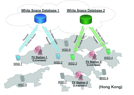
Figure 1: Illustration of a database-assisted TV white space network. To access a TV channel, each WSD first reports its location to a white space database (request), and then the database returns the available channel list to the WSD.

Figure 1 illustrates such a database-assisted TV white space network, with 3 licensed TV stations and 8 unlicensed WSDs. Here WSDs $1$ and $2$ query the available channel information from database 1, WSDs $3$ and $4$ query the available channel information from database 2, and WSDs $5$ to $8$ remain inactive (hence are not connected with any database in the figure).

The geo-location databases are usually operated by third-party companies, such as Google and SpectrumBridge. Hence, the commercial deployment of such a database-assisted network requires a proper business model, which offers sufficient incentives to the database operators to cover their capital expense (CapEx) and operating expense (OpEx). The existing business modeling of TV white space network mainly focused on the spectrum market [4, 5, 6, 7, 8], where the database operators, acting as spectrum brokers or agents, sell the TV white spaces to unlicensed WSDs for profit. However, the TV spectrum market model may not be suitable in practice due to some regulatory considerations. For example, TV white spaces (especially those not licensed to any TV stations) are usually treated as public resources, and shared by unlicensed devices. Therefore, it may not be suitable for TV white spaces to be traded in a spectrum market like other licensed spectrum bands. To this end, a new business model without involving spectrum trading is highly desirable.

The world first white space database operator certified by FCC – Spectrum Bridge – proposed an alternative business model called “White Space Plus”. The basic idea is to sell some advanced information (regarding the quality of TV channels) to WSDs, such that the latter can choose and operate on the high quality channels. An example of such information is the degree of interference on every available channel. This essentially leads to an information market, where WSDs purchase the information regarding the channel quality from the database, instead of purchasing the channel. Clearly, the successful deployment of such an information market requires (i) an accurate model to evaluate the value of information for WSDs (buyers), and (ii) a carefully designed pricing strategy for each database. However, none of these two issues has been considered in the current White Space Plus. This motivates us to study the oligopoly information market model for white space databases in this paper.

I-B Contributions

In this paper, we present and study a Model of INformation markEt for GeO-Location Database (MINE GOLD), where multiple databases (sellers) compete to sell the advanced information regarding the quality of TV channels to WSDs. The WSDs (buyers) decide whether and from which database to purchase the information. This leads to the following two-stage hierarchical model. In Stage I, each database determines the information price to WSDs. In Stage II, WSDs decide the best purchasing decisions, given the information prices of all databases. Note that the WSDs’ behaviors dynamically evolve due to the positive network externality in the information market, as more WSDs purchasing the information increases the quality/value of the database’s information and improves the WSDs performance. Such a performance change further stimulates WSDs to adjust their behaviors in the future, hence the WSDs’ behaviors dynamically evolve.

Through such a two-stage hierarchical model, we will provide insights regarding the databases’ and WSDs’ strategic decisions. Specifically, we will study the following problems systematically:

• How should each database determine the information price (in Stage I) to maximize his expected revenue, considering the competition from other databases?

• How will the WSDs’ optimal purchasing behavior (in Stage II) dynamically evolve over time, and what is the stable market shares of databases (also called market equilibrium)?

Both problems are challenging due to the following reasons. First, there is lack of a unified framework to evaluate the value of information to WSDs. In particular, one database’s known information may not be the same as the others, and no database has the global information. To this end, we propose a general framework to evaluate the value of information for WSDs. The framework considers not only the potential error of the information provided by databases, but also the heterogeneity of WSDs.

Second, the information market has the property of positive network externality, i.e., the more WSDs purchasing information from the same database, the higher value of that database’s information for each buyer. This is quite different from traditional spectrum markets which are usually congestion-oriented, i.e., the more users purchasing and using the same spectrum, the less value of spectrum for each buyer due to interferences. Here the positive correlation between the information value and market share complicates the market behavior analysis, as the change of a single WSD’s purchasing behavior may affect the information evaluation and purchasing decisions of other WSDs. We show how the market share of each database dynamically evolves over time, and what is the market equilibrium it eventually converges to.

Third, the competition among multiple databases makes the analysis even more challenging, especially when considering the positive network externality. This is different from most prior price competition analysis in the wireless literature, where the users’ decisions are either decoupled [14, 15] or negatively correlated [16]. Nevertheless, we are able to characterize the conditions for the existence and uniqueness of the price equilibrium.

As far as we know, this is the first work that systematically studies an oligopoly information market for TV white space networks. In summary, the key contributions of this paper are summarized as follows.

• Novelty and Practical Significance. We consider an oligopoly information market and propose a two-stage hierarchical business model, which captures the positive network externality of the TV white space network. Comparing with the traditional spectrum market model, this information market model better fits the regulatory requirements and industry practice.

• Market Equilibrium Analysis. We characterize the equilibrium of the proposed information market systematically. Our analysis indicates that given the prices of databases, there may be multiple market equilibria, and which one will actually emerge depends on the initial market shares of databases. We further show that some equilibria are stable, in the sense that a small fluctuation on the equilibrium will drive the market back to the equilibrium, while others are not.

• Competition among databases. We formulate the competition among databases as a price competition game, and study the existence and uniqueness of the price equilibrium. To do this, we first transform the price competition game into an equivalent market share competition game. Then we analyze the existence and uniqueness of the equilibrium of the transformed game systematically using supermodular game theory.

• Observations and Insights. Our numerical results show that, perhaps counter-intuitively, the databases’ aggregate revenue first increases and then decreases with the number of databases. Intuitively, there is a trade-off between the decreasing equilibrium prices and the increasing market shares for the databases. Extensive simulations show that having two databases will maximize the databases’ aggregate revenue under a wide range of system parameters. Moreover, our numerical results show that a large degree of positive network externality would improve the databases’ revenues and the system performance.

The rest of the paper is organized as follows. In Section II. we review the related literature. In Section III, we present the system model. In Sections IV and V, we study the monopoly and competitive network scenarios, respectively. In Section, we provide numerical results. Finally, we conclude in Section VII. We provide the detail proofs in the appendix.

II Related Work

Most of the existing studies on cognitive green communications focused on the technical issues such as spectrum sharing, resource optimization, and platform implementation [18, 19, 20]. In [18], Palicot demonstrated how to apply cognitive radio technology to achieve green radio communications. In [19], G$\ddot{u}t$ et al. studied the trade-off among energy efficiency, performance, and practicality in cognitive radio network. In [20], Ji et al. proposed a platform to explore TV white space in order to achieve green communication in cognitive radio network. However, none of the above studies considered the incentives issues in implementing such a cognitive radio network. Without a proper business model to provide sufficient incentives to the involved parties such as spectrum licensees and the network operators, it is difficult to envision strong commercialisation of this new technology.

Prior studies related to the business modeling of TV white space networks mainly focused on the spectrum trading market [4, 5, 6, 7, 8, 9]. In [4], Niyato et al. proposed a hierarchical spectrum trading model to analyze the interaction among service providers, TV licensees, and users. In [5], Luo et al. studied the (dedicated) TVWS reservation problem for a single database. In [6], Bogucka et al. discussed a spectrum trading mechanism implemented by the spectrum broker in TV white spaces. In [7], Feng et al. studied the hybrid pricing scheme for the database manager. In [9], Luo et al. discussed the price-Inventory competition game among multiple databases. The key idea of this spectrum trading market is to let the databases, acting as spectrum brokers or agents, sell the TV white spaces to WSDs for profit. However, TV spectrum trading may not always be possible as TV white spaces are sometimes considered as public spectrum resources and need to be used in a shared fashion. Some recent studies [10, 11, 12, 13] proposed the pure and hybrid information models for TV white spaces. However, these studies focused either on a single database or two competitive databases. In this work, we consider a more general oligopoly market with many competitive databases.

Price competition in a market can be modeled as a non-cooperative game. In [14], Niyato et al. studied the problem of spectrum trading with multiple licensed users selling spectrum opportunities to multiple unlicensed users, and proposed an iterative algorithm to achieve the Nash equilibrium in this competitive network. In [15], Kasbekar et al. analyzed price competition in spectrum trading market, jointly considering both bandwidth uncertainty and spatial reuse. However, in all of the above works, the market is usually assumed to be associated with the negative network externality or non-externality. In our work, as will be discussed later, the information market is associated with the positive network externality. This makes our market analysis quite different with the above works.

III System Model

We consider a database-assisted TV white space network with a set $\mathcal{M}=\{1,\ldots,M\}$ of geo-location databases and a set of $N$ unlicensed users (devices) operating on TV channels. The databases hold the list of TV licensees, update the licensees’ channel occupations information periodically, and calculate a set of available TV channels (i.e., unlicensed TV channels or those are not occupied by the licensees). The available TV channels are also called TV white spaces, which can be used by unlicensed users freely in a shared manner (e.g., using CDMA or CSMA). Each WSD queries a database for the available TV channel set, and can only operate on one of the available channels at any time.

III-A Geo-location Database

Motivated by t he current commercial examples, the database provides the following two services to the WSDs.

III-A1 Basic Service

According to the regulation policy (e.g., [2]), it is mandatory for a geo-location white space database to provide the following information for any unlicensed WSD: (i) the list of TV white spaces (i.e., unlicensed TV channels), and (ii) the transmission constraint (e.g., maximum transmission power) on each channel in the list. The database needs to provide this basic (information) service free of charge for any unlicensed user.

III-A2 Advanced Service

Beyond the basic information, each database can also provide certain advanced information regarding the quality of TV channels (as SpectrumBridge does in White Space Plus), which we call the advanced (information) service, as long as it does not conflict with the free basic service. Such an advanced information can be rather general, and a typical example is the “interference level on each channel”. With the advanced information, the WSD is able to choose a channel with the highest quality (e.g., with the lowest interference level). Hence, the database can sell this advanced information to users for profit. This leads to an information market. For convenience, let $\pi_{m}\geq 0$ denote the (advanced) information price of database $m$, $m\in\mathcal{M}$.

WSDs need to interact with databases periodically for the basic service or advanced service. The length of each interaction period (called frame) will be subject to the regulatory constraint, e.g., 15 minutes according to the latest Ofcom rule. In this work, we focus on the interactions of WSDs and databases in a particular frame, where databases announce their prices at the beginning of the frame, and then WSDs choose actions that last for the entire frame.

III-B White Space Devices

After obtaining the available channel list through the free basic service, each WSD has $M+2$ choices (denoted by $l$) in terms of channel selection:

• $l=\textsf{b}$: Inquires one database and chooses the basic service (i.e., randomly chooses an available channel) provided by the chosen database;

• $l=\textsf{s}$: Inquires one database to obtain the list of available channels and senses all the available channels to determine the best one at the cost $c$;

• $l=\textsf{m}$: Subscribes to database $m$’s advanced service, and picks the channel with the best quality indicated by database ${m}$.

Here we assume that the sensing is perfect without errors, hence a WSD can always choose the best channel when choosing the sensing service. We further denote $B$, $S$, and $A_{m}$ as the expected utility that a WSD can achieve from choosing the basic service ($l=\textsf{b}$), sensing ($l=\textsf{s}$), and the advanced service of database $m$ ($l=\textsf{m}$), respectively. As all the databases provide the same basic information (i.e., the available channel set), WSDs would achieve the same expected utility from choosing the basic service (i.e., $l=\textsf{b}$) or from choosing sensing (i.e., $l=\textsf{s}$), no matter which database they inquire. However, the expected utility from choosing different databases’ advanced services (i.e., $l=\textsf{m}$) can be different, as databases may hold different qualities of information.

The payoff of a WSD is defined as the difference between the achieved utility and the service cost (i.e., the information price when choosing the advanced service, or the sensing cost if choosing sensing by itself). Let $\theta$ denote the WSD’s evaluation for the achieved utility. Then, the payoff of a WSD with an evaluation factor $\theta$ is

$$\textstyle\Pi^{\textsc{eu}}_{\theta}=\left\{\begin{aligned} &\textstyle\theta\cdot B,&&\ \text{if}~{}l=\textsf{b},\\ &\textstyle\theta\cdot S-c,&&\ \text{if}~{}l=\textsf{s},\\ &\textstyle\theta\cdot A_{m}-\pi_{m},&&\ \text{if}~{}l=\textsf{m}.\end{aligned}\right.$$ (1)

Each WSD is rational and will choose a strategy $l\in\{\textsf{b},\textsf{s},\textsf{m}\}$ that maximizes its payoff. Note that different WSDs may have different values of $\theta$ (e.g., depending on application types), hence have different choices. That is, WSDs are heterogeneous in term of $\theta$. For convenience, we assume that $\theta$ is uniformly distributed in $[0,1]$ for all WSDs.

Let $\eta_{\textsc{b}}$, $\eta_{s}$, and $\eta_{{m}}$ denote the the fraction of WSDs choosing the basic service, sensing, and the advanced service of database $m$, respectively. For convenience, we refer the fraction of WSDs choosing particular service as the market share of such service. Obviously, $\eta_{\textsc{b}},\eta_{s},\eta_{{m}}\geq 0$ and $\eta_{\textsc{b}}+\eta_{s}+\sum_{m\in\mathcal{M}}\eta_{{m}}=1$. Hence, the payoff of the database $m\in\mathcal{M}$, which is defined as the difference between the revenue obtained by providing the advanced service and the cost, is

$$\Pi^{\textsc{db}}=(\pi_{m}-c_{m})\cdot\eta_{{m}}\cdot N,$$ (2)

where $c_{m}$ denotes database $m$’s energy consumption cost when providing the advance service to one WSD.

III-C Positive Network Externality

Note that the information market has the property of positive network externality. This is because the more WSDs subscribing to the advanced service, the more accurate the database’s information is, and further the more benefit for the WSDs subscribing to the advanced service. Next we analytically quantify this positive network externality. We first list important assumptions made in this paper to clarify the scenario on which we focus. All these assumptions have been verified to be reasonable through extensive simulations, where the advanced information is the interference level on each channel. We provide more detailed modeling and formulation for such interference information in Appendix.

Assumption 1.

$B$ and $S$ are independent of $\eta_{\textsc{b}}$, $\eta_{{m}}$, and $\eta_{s}$.

The reason for this assumption is as follows. From the system perspective, each WSD will access a channel randomly and independently. First, WSDs choosing the basic service will access one TV channel randomly. Second, WSDs choosing sensing will always access their best TV channels, and the best channels for different WSDs are independent. Hence, from the system perspective, all the WSDs will be randomly and uniformly distributed in all the channels. Hence, the utility provided by the basic service or sensing depends on the average number of WSDs in each channel, while not on the detailed numbers of WSDs using different services.

Assumption 2.

$A_{m}$ is non-decreasing in $\eta_{{m}}$.

This assumption actually reflects the positive network externality in the information market. Namely, the more users subscribing to database $m$’s advanced service, the higher quality of the database $m$’s information. For more details, please refer to Appendix.

Assumption 3.

$S\geq A_{m}\geq B$.

The reason behind $S\geq A_{m}$ is that sensing is perfect and can enable a WSD to locate the optimal TV channel. The reason behind $A_{m}\geq B$ is that WSDs can achieve additional performance gains from the advanced information provided by any database. Note that if $A_{m}<B$, then we have the trivial case that WSDs will never choose the advanced service even when the information price $\pi_{m}=0$.

For convenience, we write $A_{m}$ as a non-decreasing function of $\eta_{{m}}$, $m\in\mathcal{M}$, i.e., $A_{m}(\eta_{{m}})\triangleq g(\eta_{{m}}).$

Note that function $g(\cdot)$ reflects the performance gain induced by the advanced information, i.e., the (advanced) information value. We further introduce the following assumptions on functions $g(\cdot)$.

Assumption 4.

Function $g(\cdot)$ is non-negative, non-decreasing, concave, and continuously differentiable.

Assumption 4 results form the diminishing marginal performance improvement induced by the advanced information. Such a generic function $g(\cdot)$ can cover a wide range of application specific definitions of the advanced information, e.g., the interference level on each channel. The detailed discussion is provided in Appendix.

Stage I: Price Competition Game
Database determines the information price;
$\Downarrow$
Stage II: WSD Behaving and Market Dynamics
WSDs determine and update their best choices;
The market dynamically evolves to the equilibrium point.

Figure 2: Two-stage Interaction Model

III-D Two-Stage Interaction Model

Based on the above discussion, an information market captures the interactions among the geo-location databases and the WSDs. Hence, we formulate the interactions as a two-stage hierarchical model illustrated in Figure 2. Specifically, in Stage I, each database determines the advanced information price $\pi_{m}$. In Stage II, WSDs determine their best choices, and dynamically update their choices based on the current market shares. Accordingly, the market dynamically evolves and finally reaches the equilibrium point.

In Section IV, we will first analyze a simple monopoly information market with a single database to facilitate the understanding of this market. Then in Section V, we will analyze a more general oligopoly information market with multiple databases.

IV Monopoly Information Market

We first consider a simple monopoly scenario, where a single database provides TV white space information service to WSDs. We will denote the monopoly database as database $1$. This case study will serve as a benchmark for the later discussions of the oligopoly market in Section V. In what follows, we study the two-stage model by backward induction. Namely, we first study the WSDs’s subscription behaviour and market equilibrium in Stage II. Then, based on the market analysis, we study the monopoly database’s best pricing decision that maximizes its revenue in Stage I.

IV-A WSDs’ Best Strategy

As Assumption 2 shows that the utility provided by the advanced service of database $1$ is varying with the database’s market share, each WSD will form a belief on the utility of database $1$ and make a subscription decision. For convenience, we introduce a virtual time-discrete system with slots $t=1,2,\ldots$, where WSDs change their decisions at the beginning of every slot, based on the derived market shares in the previous slot. Let $\eta_{{1}}^{t}$ denote the market share derived at the end of slot $t$. Then we consider a WSD’s best strategy at the end of slot $t$, given the market share $\{\eta_{\textsc{b}}^{t},\eta_{s}^{t},\eta_{{1}}^{t}\}$ where $\eta_{\textsc{b}}^{t}+\eta_{s}^{t}+\eta_{{1}}^{t}=1$.

When there is only one database operating in the TV white space market, each WSD has three choices: (i) chooses the basic service by randomly choosing a channel from the available channel set, i.e., $s=\textsf{b}$, with zero cost; (ii) senses all the available channels to determine the best one, i.e., $s=\textsf{s}$ with the sensing cost $c$; and (iii) subscribes to the advanced service of the (only) database ${1}$, i.e., $s={1}$, and pays the database ${1}$ an information price $\pi_{1}$. Notice that each WSD will choose a strategy that maximizes its payoff defined in (1). Hence, given the market share $\{\eta_{\textsc{b}}^{t},\eta_{s}^{t},\eta_{{1}}^{t}\}$ with $\eta_{\textsc{b}}^{t}+\eta_{s}^{t}+\eta_{{1}}^{t}=1$, a type-$\theta$ WSD’s best strategy is

$$\textstyle\left\{\begin{aligned} &s_{\theta}^{*}=\textsf{b},\mbox{~{}~{}~{}~{}iff~{}~{}}\theta\cdot B>\max\{\theta\cdot A_{1}(\eta_{{1}}^{t})-\pi_{1},\ \theta\cdot S-c\}\\ &s_{\theta}^{*}=\textsf{s},\mbox{~{}~{}~{}~{}iff~{}~{}}\theta\cdot S-c>\max\{\theta\cdot B,\ \theta\cdot A_{1}(\eta_{{1}}^{t})-\pi_{1}\}\\ &s_{\theta}^{*}={1},\mbox{~{}~{}~{}iff~{}~{}}\theta\cdot A_{1}(\eta_{{1}}^{t})-\pi_{1}>\max\{\theta\cdot B,\ \theta\cdot S-c\}\end{aligned}\right.$$ (3)

where $A_{1}(\eta_{{1}}^{t})=g(\eta_{{1}}^{t})$, and $B<A_{1}(\eta_{{1}}^{t})<S$ based on Assumptions 1 and 2.

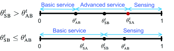
Figure 3: Illustration of $\theta_{\textsc{SB}}^{t}$, $\theta_{\textsc{AB}}^{t}$, and $\theta_{\textsc{SA}}^{t}$ in slot $t$.

To better illustrate the above best strategy, we introduce the following notations:

$$\textstyle\theta_{\textsc{SB}}^{t}\triangleq\frac{c}{S-B},~{}~{}~{}~{}\theta_{\textsc{AB}}^{t}\triangleq\frac{\pi_{1}}{A_{1}(\eta_{{1}}^{t})-B},~{}~{}~{}~{}\theta_{\textsc{SA}}^{t}\triangleq\frac{c-\pi_{1}}{S-A_{1}(\eta_{{1}}^{t})}.$$

Intuitively, $\theta_{\textsc{SB}}^{t}$ denotes the smallest $\theta$ such that a type-$\theta$ WSD prefers sensing than the basic service; $\theta_{\textsc{AB}}^{t}$ denotes the smallest $\theta$ such that a type-$\theta$ WSD prefers the advanced service than the basic service; and $\theta_{\textsc{SA}}^{t}$ denotes the smallest $\theta$ such that a type-$\theta$ WSD prefers sensing than the advanced service. Notice that $A_{1}(\eta_{{1}}^{t})$ is a function of the market share $\eta_{{1}}^{t}$. Hence, $\theta_{\textsc{AB}}^{t}$ and $\theta_{\textsc{SA}}^{t}$ are also functions of $\eta_{{1}}^{t}$.

Figure 3 illustrates two possible relationships of $\theta_{\textsc{SB}}^{t}$, $\theta_{\textsc{AB}}^{t}$, and $\theta_{\textsc{SA}}^{t}$. Intuitively, Figure 3 implies that WSDs with a high utility evaluation factor $\theta$ are more willing to choose sensing in order to achieve the maximum utility. WSDs with a low utility evaluation factor $\theta$ are more willing to choose the basic service, so that they will pay zero cost. WSDs with a middle utility evaluation factor $\theta$ are willing to choose the advanced service, in order to achieve a relatively large utility with a relatively low service cost. Notice that when the information price $\pi_{1}$ is high or the information value (i.e., $A_{1}(\eta_{{1}}^{t})-B$) is low, we could have $\theta_{\textsc{SB}}^{t}<\theta_{\textsc{AB}}^{t}$, in which no users will choose the advanced service (as illustrated in the lower subfigure of Figure 3).

Next we characterize the market shares in slot $t+1$, resulting from the WSDs’ best choices in slot $t$. Such derived market shares are important for analyzing the market evolution in the next subsection. Assume that all WSDs update the best strategies once and simultaneously. Recall that $\theta$ is uniformly distributed in $[0,1]$. Then, given any market share $\eta_{{1}}^{t}$ in slot $t$, the market share $\eta_{{1}}^{t+1}$ in slot $t+1$ is

• If $\theta_{\textsc{SB}}^{t}>\theta_{\textsc{AB}}^{t}$, then $\eta_{{1}}^{t+1}=\theta_{\textsc{SA}}^{t}-\theta_{\textsc{AB}}^{t}$;

• If $\theta_{\textsc{SB}}^{t}\leq\theta_{\textsc{AB}}^{t}$, then $\eta_{{1}}^{t+1}=0$.

Formally, we have the following market share in slot $t+1$.

Lemma 1.

Given database ${1}$’s market share $\eta_{{1}}^{t}$ at the end of slot $t$, the market share $\eta_{{1}}^{t+1}$ in slot $t+1$ is given by

$$\eta_{{1}}^{t+1} =\max\big{\{}\min\{\theta_{\textsc{SA}}^{t},1\}-\theta_{\textsc{AB}}^{t},\ 0\big{\}}.$$ (4)

As $\theta_{\textsc{AB}}^{t}$ and $\theta_{\textsc{SA}}^{t}$ are functions of the market share $\eta_{{1}}^{t}$, the market share $\eta_{{1}}^{t+1}$ in slot $t+1$ is also a function of $\eta_{{1}}^{t}$, and hence can be written as $\eta_{{1}}^{t+1}(\eta_{{1}}^{t})$.

IV-B Market Dynamics and Equilibrium

When the market share of database $1$ changes, the WSDs’ payoffs (when choosing the advanced service) change accordingly, as $A_{1}(\eta_{{1}}^{t})$ changes. As a result, WSDs will update their best strategies continuously, hence the market shares will evolve dynamically, until reaching a stable point (called market equilibrium). In this subsection, we will study such a market dynamics and equilibrium, under a fixed price $\pi_{1}$.

Base on analysis in Section IV-A, let $\eta_{{1}}^{0}$ denote the initial market share in slot $t=0$ and $\eta_{{1}}^{t}$ denote the market share derived at the end of slot $t$. We further denote $\triangle\eta_{{1}}$ as the change of market share between two successive time slots, e.g., $t$ and $t+1$, that is,

$$\triangle\eta_{{1}}(\eta_{{1}}^{t}) =\eta_{{1}}^{t+1}-\eta_{{1}}^{t},$$ (5)

where $\eta_{{1}}^{t+1}$ is the derived market share in slot $t+1$, which can be computed by Lemma 1. Obviously, if $\triangle\eta_{{1}}$ is zero in slot $t+1$, i.e., $\eta_{{1}}^{t+1}=\eta_{{1}}^{t}$, then WSDs will no longer change their strategies in the future. This implies that the market achieves a stable state, which we call the market equilibrium. Formally,

Definition 1 (Monopoly Market Equilibrium).

A market share $\eta_{{1}}^{t}$ in slot $t$ is a market equilibrium iff

$$\triangle\eta_{{1}}(\eta_{{1}}^{t})=0.$$ (6)

Definition 1 implies that once the market share satisfies (6) in slot $t$, the market share remains the same from that time slot on. For notational convenience, we will also denote the market equilibrium by $\eta_{{1}}^{*}$.

Next, we study the existence of the market equilibrium, and further characterize the market equilibrium analytically. Specifically, we will show that under a fixed price $\pi_{1}$, there may be multiple equilibria, and which one will eventually emerge depends on database’s initial market share (i.e., market share in slot $t=0$). Besides, some equilibria are stable in the sense that a small fluctuation around these equilibria will not drive the market share away from the equilibria, while some equilibria are unstable in the sense that a tiny fluctuation on these equilibria will drive the market share to a different equilibrium.

Proposition 1 (Existence).

Given any fixed price $\pi_{1}$ and sensing cost $c$, there exists at least one market equilibrium.

Proposition 2 (Uniqueness).

Given any fixed price $\pi_{1}$ and sensing cost $c$, there exists a unique market equilibrium $\eta_{{1}}^{*}$ if

$$\textstyle\max_{\eta_{{1}}\in[0,1]}\frac{A_{1}^{\prime}(\eta_{{1}})}{A_{1}(\eta_{{1}})-B}\cdot\frac{S-B}{S-A_{1}(\eta_{{1}})}\leq\kappa_{2},$$ (7)

where $\kappa_{2}=1/{\max_{\eta_{{1}}\in[0,1]}\theta_{\textsc{SA}}(\eta_{{1}})}$.

Recall that $g(\eta_{{1}})$ is concave in $\eta_{{1}}$ and $A_{1}(\eta_{{1}})=g(\eta_{{1}})$ by Assumption 4. Hence, a practical implication of (7) is that if the information value $A_{1}(\eta_{{1}})$ (i.e., the positive network externality) increases slowly with $\eta_{{1}}$, then there exists a unique equilibrium. Note that the condition (7) is sufficient but not necessary for the uniqueness. Simulations show that the market converges to a unique equilibrium for a wide range of prices, under which the condition (7) can be violated. Nevertheless, the condition in (7) leads to the insight that if the change of positive network externality is slow, there exists a unique equilibrium point.

Suppose the uniqueness condition (7) is satisfied. Let $A_{1}^{\text{min}}$ be the minimum expected utility that a WSD can achieve from choosing the advanced service of monopoly database $1$. Correspondingly, let $\theta_{\textsc{AB}}^{\text{max}}=\frac{\pi_{1}}{A_{1}^{\text{min}}-B}$ be the corresponding value when $A_{1}=A_{1}^{\text{min}}$. We characterize the unique equilibrium by the following theorem.

Theorem 1 (Market Equilibrium).

Suppose the uniqueness condition (7) holds. Then, for any price $\pi_{1}$ and sensing cost $c$, the unique market equilibrium is given by

• If $\theta_{\textsc{AB}}^{\text{max}}<\theta_{\textsc{SB}}$, then there is a unique market equilibrium $\eta_{{1}}^{*}$ given by

  $$\textstyle\eta_{{1}}^{*}=\min\{\theta_{\textsc{SA}}(\eta_{{1}}^{*}),1\}-\theta_{\textsc{AB}}(\eta_{{1}}^{*}).$$ (8)

• If $\theta_{\textsc{AB}}^{\text{max}}\geq\theta_{\textsc{SB}}$, then there is a unique market equilibrium $\eta_{{1}}^{{\dagger}}$ given by

  $$\textstyle\eta_{{1}}^{{\dagger}}=0.$$ (9)

Theorem 1 shows that if the information value (i.e., $A_{1}^{\text{min}}-B$) is low, then $\theta_{\textsc{AB}}^{\text{max}}\geq\theta_{\textsc{SB}}$ and no WSDs will choose the advanced service in the market equilibrium. Only when the information value is high enough (i.e., $\theta_{\textsc{AB}}^{\text{max}}<\theta_{\textsc{SB}}$ ), the database $1$ can obtain the positive market equilibrium.

IV-C Revenue Maximization

Based on the market equilibrium analysis in the previous subsection, we will study the optimal information pricing strategy of the monopoly database ${1}$ that maximizes its payoff, i.e.,

$$\Pi^{\textsc{db}}_{1}(\pi_{1})=(\pi_{1}-c_{1})\cdot\eta_{{1}}^{*}(\pi_{1})$$ (10)

where $c_{1}$ is the operational cost of the database that characterizes the energy consumption of the database to provide the advanced service, and $\eta_{{1}}^{*}$ is the equilibrium point of the WSD subscription dynamics at price $\pi_{1}$ given by Theorem 1.

Directly solving the optimal price that maximizes (10) is very challenging, due to the difficulty in analytically characterizing the market equilibrium $\eta_{{1}}(\pi_{1})$ under a particular price pair $\pi_{1}$. To this end, we transform the original price maximization problem into an equivalent market share maximization problem. The key idea is to view the market share as the strategy of the database, and the price as a function of the market share.

Furthermore, under the uniqueness condition (7), there is a one-to-one correspondence between the market equilibrium $\eta_{{1}}^{*}$ and the prices $\pi_{1}$. In this sense, once the monopoly database ${1}$ chooses the prices $\pi_{1}$, it has equivalently chosen the market share $\eta_{{1}}^{*}$ (given the fixed sensing cost). Hence, we obtain the equivalent market share maximization problem, where the strategy of the database is its market share (i.e., $\eta_{{1}}$), and the prices $\pi_{1}$ is the function of the market share $\eta_{{1}}$. Let $A_{1}^{\text{max}}$ be the maximum expected utility that a WSD can achieve from choosing the advanced service of monopoly database $1$, i.e., when all WSDs choose database $1$’s advanced service. Then substitute $\theta_{\textsc{SA}}=\frac{c-\pi_{1}}{S-A_{1}(\eta_{{1}})}$ and $\theta_{\textsc{AB}}=\frac{\pi_{1}}{A_{1}(\eta_{{1}})-B}$ into (8) and (9), we can derive the inverse function of (8) and (9), where price is a function of market share, i.e.,

• Low sensing cost: $c<S-A_{1}^{\text{max}}$,

  $$\textstyle\pi_{1}(\eta_{{1}})=\frac{S-A_{1}(\eta_{{1}})}{S-B}\cdot\big{(}\frac{c}{S-A_{1}(\eta_{{1}})}-\eta_{{1}}\big{)}\cdot\big{[}A_{1}(\eta_{{1}})-B\big{]}.$$ (11)

• High sensing cost: $c\geq S-A_{1}^{\text{max}}$,

  $$\textstyle\pi_{1}(\eta_{{1}})=(1-\eta_{{1}})\cdot\big{[}A_{1}(\eta_{{1}})-B\big{]}.$$ (12)

Accordingly, the revenue of the monopoly database can be written as:

$$\textstyle\Pi^{\textsc{db}}_{1}(\eta_{{1}})=(\pi_{1}(\eta_{{1}})-c_{1})\cdot\eta_{{1}}$$ (13)

We first show the equivalence between the price maximization problem and the market share maximization problem.

Proposition 3 (Equivalence).

If $\eta^{*}$ is an optimal solution of (13), then $\pi_{1}^{*}$ calculated by substituting $\eta^{*}$ into (11) or (12) is an optimal solution of (10).

We can easily check that the database’s revenue in (13) is monotonic in $\eta_{{1}}\in[0,1]$, hence we have:

Proposition 4 (Optimal Information Pricing).

There exists a unique optimal solution $\pi_{1}^{*}$ for the database, where for

• low sensing cost: $c<S-A_{1}^{\text{max}}$,

  $$\textstyle\pi_{1}^{*}\triangleq\frac{S-A_{1}(\eta_{{1}}^{{\dagger}})}{S-B}\cdot\big{(}\frac{c}{S-A_{1}(\eta_{{1}}^{{\dagger}})}-\eta_{{1}}^{{\dagger}}\big{)}\cdot\big{[}A_{1}(\eta_{{1}}^{{\dagger}})-B\big{]},$$ (14)

• high sensing cost: $c\geq S-A_{1}^{\text{max}}$,

  $$\textstyle\pi_{1}^{*}\triangleq(1-\eta_{{1}}^{{\ddagger}})\cdot\big{[}A(\eta_{{1}}^{{\ddagger}})-B\big{]},$$ (15)

where $\eta_{{1}}^{{\dagger}}$ is the solution of $\textstyle\frac{A_{1}(\eta_{{1}})-B}{S-B}c+\big{(}\frac{c}{S-B}+\frac{2A_{1}(\eta_{{1}})-S-B}{S-B}\eta_{{1}}\big{)}\frac{\mathrm{d}A(\eta_{{1}})}{\mathrm{d}\eta_{{1}}}\eta_{{1}}-2\eta_{{1}}\frac{S-A_{1}(\eta_{{1}})}{S-B}\big{[}A_{1}(\eta_{{1}})-B\big{]}-c_{1}=0,$ and $\textstyle\eta_{{1}}^{{\ddagger}}$ is the solution of $\textstyle A(\eta_{{1}})-B+\frac{(1-\eta_{{1}})\cdot\eta_{{1}}}{1-2\eta_{{1}}}\cdot\frac{\mathrm{d}A(\eta_{{1}})}{\mathrm{d}\eta_{{1}}}-\frac{c_{1}}{1-2\eta_{{1}}}=0$.

V Oligopoly Information Market

In this section, we study the general competition scenario, where $M$ databases compete for selling information to the same pool of WSDs. In such an oligopoly information market, $M$ databases (the leaders) first choose their own information prices independently. Then, WSDs (the followers) subscribe to different services accordingly. Similar as in the monopoly scenario, we will study the oligopoly information market by backward induction.

V-A Stage II - Users Behavior and Market Equilibrium

Similar as in Sections IV-A and IV-B, we study the WSD behavior and market dynamics in this section, given the databases’ information prices $\pi_{m}$, $m\in\mathcal{M}$, and the sensing cost $c$.

We first consider a WSD’s best strategy at the end of slot $t$, where the market shares are $\{\eta_{\textsc{b}}^{t},\eta_{s}^{t},\eta_{{m}}^{t}\}$ with $\eta_{\textsc{b}}^{t}+\eta_{s}^{t}+\sum_{m=1}^{M}\eta_{{m}}^{t}=1$. A type-$\theta$ WSD at the time slot $t+1$ will
(i) subscribes to the basic service and randomly chooses a channel, i.e., $s_{\theta}^{*}=\textsf{b}$, iff

$$\theta\cdot B>\max\{\theta\cdot S-c,\ \ \max_{m\in M}(\theta\cdot A_{m}(\eta_{{m}}^{t})-\pi_{m})\},$$ (16)

(ii) senses all the available channels to determine the best one, i.e., $s_{\theta}^{*}=\textsf{s}$, iff

$$\theta\cdot S-c>\max\{\theta\cdot B,\ \ \max_{m\in M}(\theta\cdot A_{m}(\eta_{{m}}^{t})-\pi_{m})\},$$ (17)

(iii) subscribes to the database ${m}$’s advanced service, i.e., $s_{\theta}^{*}=\textsf{m}$, iff

$$\theta\cdot A_{m}(\eta_{{m}}^{t})-\pi_{m}> \max\{\theta\cdot B,\ \ \theta\cdot S-c,\max_{n\in M,n\neq m}(\theta\cdot A_{n}(\eta_{n}^{t})-\pi_{n})\},$$ (18)

where $m=1,2,\ldots,M$.

Without loss of generality, we suppose that the market shares of $M$ databases in time slot $t$ are ordered as: $\eta_{{M}}^{t}>\eta_{{M-1}}^{t}>\ldots>\eta_{{1}}^{t}$, and accordingly, we have: $S>A_{M}(\eta_{{M}}^{t})>A_{M-1}(\eta_{{M-1}}^{t})>\ldots>A_{1}(\eta_{{1}}^{t})$. Notice that no WSD would like to choose a service with a lower QoS and a higher price. Therefore, we will consider the non-trivial scenario with $c>\pi_{M}>\pi_{M-1}>\ldots>\pi_{1}$.

To better illustrate the best strategy in (16)-(18), we introduce the following notations:

$$\theta_{\textsc{S}}^{t}\triangleq\frac{c-\pi_{M}}{S-A_{M}(\eta_{{M}}^{t})},~{}~{}~{}~{}\theta_{\textsc{B}}^{t}\triangleq\frac{\pi_{1}}{A_{1}(\eta_{{1}}^{t})-B},~{}~{}~{}~{}\theta_{{m}}^{t}\triangleq\frac{\pi_{m}-\pi_{m-1}}{A_{m}(\eta_{{m}}^{t})-A_{m-1}(\eta_{m-1}^{t})},\ m=2,3,...,M,$$

where $\theta_{\textsc{S}}^{t}$ denotes the marginal WSD who is indifferent between sensing all the available channels or subscribing to the advanced service of database ${M}$; $\theta_{\textsc{B}}^{t}$ denotes the marginal WSD who is indifferent between randomly choosing a channel or subscribing to the advanced service of database ${1}$; and $\theta_{{m}}^{t}$ denotes the marginal WSD who is indifferent between subscribing to the advanced service of database ${m}$ or database ${m-1}$.

Next we characterize the market shares in slot $t+1$, resulting from the WSDs’ best choices in slot $t$. We assume that all WSDs update the best strategies once and simultaneously. Recall that $\theta$ is uniformly distributed in $[0,1]$. Then, we have the following market shares in slot $t+1$.

Lemma 2.

Given market shares $\{\eta_{{1}}^{t},\eta_{{2}}^{t},\ldots,\eta_{{M}}^{t}\}$ in slot $t$ with $\eta_{{M}}^{t}>\eta_{{M-1}}^{t}>\ldots>\eta_{{1}}^{t}$, the newly market shares in slot $t+1$ are:

$$\left\{\begin{aligned} \eta_{{M}}^{t}&=\theta_{\textsc{S}}^{t}-\theta_{{M}}^{t},\\ \eta_{{m}}^{t}&=\theta_{{m+1}}^{t}-\theta_{{m}}^{t},\ m=2,3,\ldots,M-1\\ \eta_{{1}}^{t}&=\theta^{t}_{2}-\theta_{\textsc{B}}^{t}.\end{aligned}\right.$$ (19)

For notational convenience, we denote $\boldsymbol{\eta}_{\textsc{a}}^{t}=(\eta_{{1}}^{t},\ldots,\eta_{{M}}^{t})$ as the vector of all databases’ market shares in slot $t$. Besides, we denote $\boldsymbol{\eta}_{-m}^{t}=(\eta_{{1}}^{t},\ldots,\eta_{{m-1}}^{t},\eta_{{m+1}}^{t},\ldots,\eta_{{M}}^{t})$ as the market shares vector of all databases except database ${m}$. We also denote $\boldsymbol{\eta}_{\textsc{a}}^{0}$ as the initial market share in slot $t=0$. As $\theta_{\textsc{S}}^{t}$, $\theta_{\textsc{B}}^{t}$, and $\theta_{{m}}^{t}$ are functions of the market shares $\boldsymbol{\eta}_{\textsc{a}}^{t}$, the market shares $\boldsymbol{\eta}_{\textsc{a}}^{t+1}$ in the next slot $t+1$ are also functions of $\boldsymbol{\eta}_{\textsc{a}}^{t}$. and hence can be written as $\eta_{{m}}^{t+1}(\boldsymbol{\eta}_{\textsc{a}}^{t})$, $\forall m\in\mathcal{M}$. We further let $\triangle\eta_{{m}}$ as the change of database ${m}$’s market share between two successive time slots, e.g., $t$ and $t+1$, that is,

$$\textstyle\triangle\eta_{{m}}(\boldsymbol{\eta}_{\textsc{a}}^{t}) =\eta_{{m}}^{t+1}(\boldsymbol{\eta}_{\textsc{a}}^{t})-\eta_{{m}}^{t},$$ (20)

where $\eta_{{m}}^{t+1}$ is the derived market share of the database $m\in\mathcal{M}$ in slot $t+1$, which can be computed by Lemma 2. Then we give the definition of an equilibrium point, which is similar to Definition 1.

Definition 2 (Oligopoly Market Equilibrium).

A set of market shares $\boldsymbol{\eta}^{t}$ in slot $t$ is a market equilibrium iff

$$\triangle\eta_{{m}}(\boldsymbol{\eta}_{\textsc{a}}^{t})=0,\forall m\in\mathcal{M}.$$ (21)

Definition 2 implies that once the market shares set satisfy (21) in slot $t$, the market share set remains the same from that time slot on. We will denote the market equilibrium by $\boldsymbol{\eta}_{\textsc{a}}^{*}$.

Based on the Definition 2, we can characterize the equilibrium by the following theorem.

Theorem 2 (Market Equilibrium).

For any prices set $\{\pi_{m}\}_{m\in\mathcal{M}}$ and WSDs’ sensing cost $c$, the market equilibrium is given by:

$$\left\{\begin{aligned} \eta_{{M}}^{*}&=\theta_{\textsc{S}}(\boldsymbol{\eta}_{\textsc{a}}^{*})-\theta_{{M}}(\boldsymbol{\eta}_{\textsc{a}}^{*}),\\ \eta_{{m}}^{*}&=\theta_{{m+1}}(\boldsymbol{\eta}_{\textsc{a}}^{*})-\theta_{{m}}(\boldsymbol{\eta}_{\textsc{a}}^{*}),m=2,3,\ldots,M-1\\ \eta_{{1}}^{*}&=\theta_{2}(\boldsymbol{\eta}_{\textsc{a}}^{*})-\theta_{\textsc{B}}(\boldsymbol{\eta}_{\textsc{a}}^{*}).\end{aligned}\right.$$ (22)

Proving the uniqueness of maker equilibrium is challenging due to the difficulty in anaylzing (22). However, extensive simulations show that, even if there exist multiple market share equilibrium points, the market always converges to a unique one under fixed initial market shares. Hence, we have the following proposition which is important in analyzing the price competition game in Stage I.

Proposition 5.

Given the initial market shares (i.e., the market shares achieved in slot $t=0$), the market always converges to a unique market share equilibrium.

V-B Stage I - Price Competition Game Equilibrium

In this section, we study the interaction among $M$ databases in Stage I. Specifically, in this section we will formulate the interactions among databases as a price competition game, and study the Nash equilibrium systematically.

We first define the price competition game (PCG), denoted by $\Gamma=(\mathcal{M},\{\pi_{m}\}_{m\in\mathcal{M}},\{\Pi^{\textsc{db}}_{m}\}_{m\in\mathcal{M}})$, where

• $\mathcal{M}$ is the set of game players (databases);

• $\pi_{m}$ is the strategy of database $m$, where $\pi_{m}\geq 0$;

• $\Pi^{\textsc{db}}_{m}$ is the revenue of database $m$ defined in (2).

For notational convenience, we denote $\boldsymbol{\pi}=(\pi_{1},\ldots,\pi_{M})$ as the vector of all databases’ information prices. Besides, we denote $\boldsymbol{\pi}_{-m}=(\pi_{1},\ldots,\pi_{m-1},\pi_{m+1},\ldots,\pi_{M})$ as the price vectors of all databases except $m$. We also write the (assuming unique) market equilibrium $\boldsymbol{\eta}^{*}=\{\eta_{{1}}^{*},\ldots,\eta_{{M}}^{*}\}$ in Stage II as functions of prices $\boldsymbol{\pi}=\{\pi_{1},\ldots,\pi_{M}\}$, i.e., $\boldsymbol{\eta}^{*}(\boldsymbol{\pi})$. Intuitively, we can interpret $\eta_{{m}}^{*}(\cdot)$ as the demand functions of database $m$. Moreover, the database $m$’s market share $\eta_{{m}}$ depends not only on its own price $\pi_{m}$, but also on other databases’ price $\boldsymbol{\pi}_{-m}$. By (2), the revenue of the database $m$ is:

$$\Pi^{\textsc{db}}_{m}(\pi_{m},\boldsymbol{\pi}_{-m}) =(\pi_{m}-c_{m})\cdot\eta_{{m}}^{*}(\pi_{m},\boldsymbol{\pi}_{-m}).$$ (23)

Definition 3 (Price Equilibrium).

A price profile $\{\pi_{m}^{*}\}_{m\in\mathcal{M}}$ is called a price equilibrium, if

$$\pi_{m}^{*} =\arg\max_{\pi_{m}\geq 0}\ \Pi^{\textsc{db}}_{m}(\pi_{m},\boldsymbol{\pi}_{-m}^{*}),~{}~{}\forall m\in\mathcal{M}$$ (24)

Directly solving the price equilibrium in (24) is very challenging, due to the difficulty in analytically characterizing the market equilibrium $\{\boldsymbol{\eta}_{\textsc{a}}^{*}(\boldsymbol{\pi})\}$ under a particular price pair $\boldsymbol{\pi}$. Hence, we transform the price competition game (PCG) into an equivalent market share competition game (MSCG). The key idea is to view the market shares as the strategy of databases, and the prices as functions of the market shares.

Based on Proposition 5, there is a one-to-one correspondence between the market equilibrium $\{\boldsymbol{\eta}_{-m}^{*}\}$ and the prices $\{\boldsymbol{\pi}\}$ given fixed the initial market shares. In this sense, once the databases choose the prices $\{\pi_{m}\}_{m\in\mathcal{M}}$, they have equivalently chosen the market shares $\{\boldsymbol{\eta}_{-m}^{*}\}_{m\in\mathcal{M}}$. Hence, we obtain the equivalent market share competition game—MSCG, where the strategy of each player is its market share (i.e., $\eta_{{m}}$ for the database $m$), and the prices $\{\pi_{m}\}_{m\in\mathcal{M}}$ are functions of the market shares $\{\eta_{{m}}\}_{m\in\mathcal{M}}$. Substitute $\theta_{\textsc{S}}\triangleq\frac{c-\pi_{M}}{S-A_{M}(\boldsymbol{\eta}_{-m})}$, $\theta_{\textsc{B}}\triangleq\frac{\pi_{1}}{A_{1}(\boldsymbol{\eta}_{-m})-B}$, and $\theta_{{m}}\triangleq\frac{\pi_{m}-\pi_{m-1}}{A_{m}(\boldsymbol{\eta}_{-m})-A_{m-1}(\boldsymbol{\eta}_{-m})}$ into (22), we can derive the inverse function of (22) by recursion, where prices are functions of market shares, i.e.,

$$\pi_{m}=\sum_{m=1}^{M+1}\bigg{[}\big{(}1-\sum_{n=m}^{M+1}\eta_{n}\big{)}\cdot(g(\eta_{m})-g(\eta_{m-1}))\bigg{]}$$ (25)

where $\eta_{M+1}=\eta_{s}$, $g(\eta_{M+1})=S$, and $g(\eta_{0})=B$.

Accordingly, the revenue of database $m\in\mathcal{M}$ is:

$$\widetilde{\Pi}^{\textsc{db}}_{m}(\eta_{{m}},\boldsymbol{\eta}_{-m}) =(\pi_{m}(\eta_{{m}},\boldsymbol{\eta}_{-m})-c_{m})\cdot\eta_{{m}}.$$ (26)

Similarly, a pair of market shares $\{\eta_{{m}}^{*}\}_{m\in\mathcal{M}}$ is called a Nash equilibrium of MSCG, if

$$\eta_{{m}}^{*}=\arg\max_{\eta_{{m}}}\widetilde{\Pi}^{\textsc{db}}_{m}(\eta_{{m}},\boldsymbol{\eta}_{-m}^{*}),~{}\forall m\in\mathcal{M}.$$

We first show that the equivalence between the original PCG and the above MSCG.

Proposition 6 (Equivalence).

If $\boldsymbol{\eta}_{\textsc{a}}^{*}$ is a Nash equilibrium of MSCG, then $\boldsymbol{\pi}^{*}$ given by (25) is a Nash equilibrium of the original price competition game PCG.

We can check that $\widetilde{\Pi}^{\textsc{db}}_{m}(\eta_{{m}},\boldsymbol{\eta}_{-m})$ for $m\in\mathcal{M}$ is a decreasing differential function. Hence, under duopoly databases scenario (with two databases), the MSCG is a supermodular game (with a straightforward strategy transformation), and hence the market share equilibrium of MSCG can be easily obtained by using the supermodular game theory [21].

Lemma 3 (Existence of Market Equilibrium under Duopoly Scenario).

A duopoly MSCG is a supermodular game with respect to $\eta_{1}$ and $-\eta_{2}$. Hence, there exists at least one market share equilibrium.

Note that the MSCG under oligopoly scenario (i.e., the number of databases $M\geq 3$) cannot be transformed into supermodular game. In order to study oligopoly scenario, we consider a special case where the positive network externality of database $m\in\mathcal{M}$ is characterized as

$$g(\eta_{m})=\alpha_{m}+(\beta_{m}-\alpha_{m})\cdot{\eta_{m}}^{\gamma_{m}},$$ (27)

where $\gamma_{m}\in(0,1]$. Then we can show that $\widetilde{\Pi}^{\textsc{db}}_{m}(\eta_{{m}},\boldsymbol{\eta}_{-m})$ under function $g_{m}$ is quasiconcave in $\eta_{{m}}$. This is sufficient for guaranteeing a pure-strategy Nash equilibrium [22].

The reasons that we use (27) to characterize the positive network externality are as follows. $\alpha_{m}$ denotes the minimum benefit brought by the database $m$’s knowledge of licensees’ channel occupation information, and $\beta_{m}$ denotes the maximum benefit brought by the database’s advanced information. The parameter $\gamma_{m}\in(0,1]$ characterizes the elasticity of the network externality. Note that this function generalizes the linear network externality models in many existing literatures such as [23].

Proposition 7 (Existence of Market Equilibrium under Oligopoly Scenario).

Given the positive network externally function (27), the revenue function $\widetilde{\Pi}^{\textsc{db}}_{m}(\eta_{{m}},\boldsymbol{\eta}_{-m})$, $\forall m\in\mathcal{M}$ in MSCG is quasi-concave in $\eta_{{m}}$. Hence, there exists a pure-strategy Nash equilibrium $\boldsymbol{\eta}_{\textsc{a}}^{*}$.

Proof of Proposition 7 is similar to the analysis of the price competition game model in [24].

We then apply the contraction mapping method to establish the uniqueness of the Nash equilibrium under both duopoly and oligopoly scenarios. By applying the contraction mapping approach, the uniqueness is assured when the following condition is satisfied [25]:

$$\textstyle-\frac{\partial^{2}{\widetilde{\Pi}^{\textsc{db}}_{m}(\eta_{{m}},\boldsymbol{\eta}_{-m})}}{\partial{(-{\eta_{{m}}})}^{2}}\geq\sum_{j\neq m}\frac{\partial^{2}{\widetilde{\Pi}^{\textsc{db}}_{m}(\eta_{{m}},\boldsymbol{\eta}_{-m})}}{\partial{{(-\eta_{{m}})}}\partial{\eta_{{n}}}},\ \forall m\in\mathcal{M}.$$ (28)

We can check that the MSCG game under both duopoly and oligopoly scenarios given $g_{m}=\alpha_{m}+(\beta_{m}-\alpha_{m})\cdot{\eta_{m}}^{\gamma_{m}}$ satisfies the above condition. Hence, we have:

Proposition 8 (Uniqueness under Both Duopoly and Oligopoly Scenarios).

Given the positive network externally function (27), The MSCG with $M\geq 2$ databases has a unique Nash equilibrium $\boldsymbol{\eta}_{\textsc{a}}^{*}$.

Once we obtain the Nash equilibrium $\boldsymbol{\eta}_{\textsc{a}}^{*}$ of MSCG, we can immediately obtain the Nash equilibrium $\boldsymbol{\pi}^{*}$ of the original PCG by (25). Notice that we may not be able to derive the analytical Nash equilibrium of MSCG, as we use the generic function $g(\cdot)$. Nevertheless, because the objective function of database $m$, $m\in\mathcal{M}$ is quasiconcave, we can numerically compute the Nash equilibrium of MSCG through several standard algorithms such as the ellipsoid algorithm in [26].

VI Numerical Results

In this section, we numerically illustrate the NE of the database competition game, and evaluate the system performance (e.g., the network profit and the databases’ revenue) at the NE. We will focus on the impact of system parameters (i.e. the number of databases, the network effect, the positive network externality, and the database’s operational cost) on system performance. As a concrete example, we will use (27) to model the positive network externality. Unless specified otherwise, we assume that $B=2$, $S=8$, $\alpha_{m}=4.8$, and $\beta_{m}=6$, $m\in\mathcal{M}$. The databases’ initial market shares satisfy $\eta_{M}>\eta_{M-1}>\ldots>\eta_{1}$. In all the simulation figures, we denote sensing service as S, basic service as B, and database $m\in\mathcal{M}$ as $m$.

VI-A System Performance vs Number of Databases

Figure 4 illustrates (a) market share equilibrium, (b) price equilibrium, and (c) the system performance achieved under different numbers of databases ($M$ from $1$ to $5$). In this simulation, we fix the sensing cost as $c=2$, the network externality impact as $\gamma_{m}=0.4$, and the database’s operation cost as $c_{m}=0$, $m\in\mathcal{M}$.

Figure 4.a shows the price equilibrium achieved under different numbers of databases. We can see that the equilibrium prices decrease with the number of databases, as the intensity of competition increases. When the number of databases increases, the difference among the databases’ initial market shares becomes smaller as $\sum_{m\in M}\eta_{m}=1$. Hence, the difference among databases’ price equilibrium also decreases as $M$ becomes large.

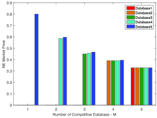
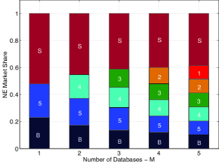
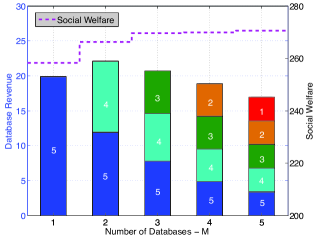
Figure 4: (a) Price equilibrium, (b) Market share equilibrium, (c) The system performance vs the number of databases.

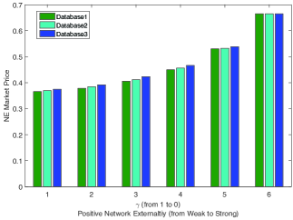
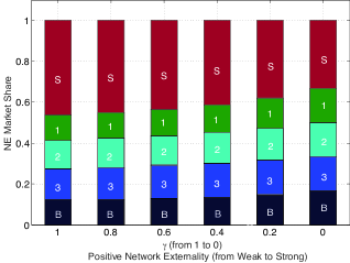
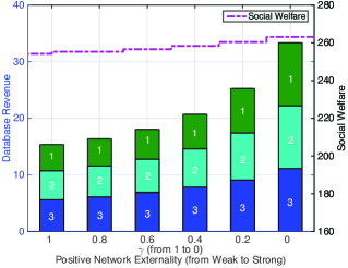
Figure 5: (a) Price equilibrium, (b) Market share equilibrium, (c) The system performance vs positive network externality. A small value of $\gamma$ corresponds to a high level of positive network externality.

Figure 4.b shows the equilibrium market share under different numbers of databases. Each bar denotes the market shares of the basic service (denoted as “B”), databases’ advanced services (denoted as the database index $m$), and sensing (denoted as “S”). We can see that the databases’ market shares increase with the number of databases. As databases’ equilibrium prices decrease with the number of databases, more WSDs will purchase the advanced services, hence increasing the market shares of the databases as $M$ increases.

Figure 4.c shows each database’s revenue and the total social welfare (i.e., the total revenue of all databases plus the total payoffs of WSDs) achieved at the NE, given different numbers of databases. Each bar denotes the aggregated revenue of $M$ databases, while each sub-bar corresponds to the payoff of database $m$. The dash red line denotes the value of social welfare. The left y-axis denotes the value of databases’ revenues, and the right y-axis denotes the value of social welfare.

From Figure 4.c, we can see that the databases’ aggregated revenue is a quasi-concave (i.e., first increasing and then decreasing) function of the number of databases $M$. This is because two things happen when $M$ increases: (i) more intensive competition drives the equilibrium prices down for all databases, which reduces the revenue of each single database, (ii) low prices attract more WSDs to purchase the advanced services, which leads to the increase the overall databases’ revenue. In this simulation, $M=2$ achieves the best trade-off and maximizes the databases’ total revenue.

Figure 4.c shows that the social welfare increases with the number of databases. As the competition among databases reduce the equilibrium prices, more WSDs choose to use the advanced services, which offers a better quality of service than the basic service and a lower cost than the sensing. Overall this improves the social welfare.

VI-B System Performance vs Network Externality

Figure 5 illustrates (a) market share equilibrium, (b) price equilibrium, and (c) the system performance achieved under different levels of network externality (e.g., $\gamma_{1}=\gamma_{2}=\gamma_{3}=\gamma$ changes from $1$ to $0$, hence the positive network externality changes from weak to strong). According to (27), a small $\gamma_{m}$ means that the value of $g(\eta_{m})$ can be reasonably large even with a small $\eta_{m}$. Hence, a small value of $\gamma$ represents a high level of network externality. In this simulation, we fix the sensing cost as $c=2$, the number of database $M=3$, and the database’s operation cost as $c_{m}=0$, $m\in\mathcal{M}$.

Figure 5.a shows the equilibrium prices of positive network externality. We can see that the databases’ equilibrium prices increases with the level of network externality. This is because a higher level of positive network externality will make the utility provided by the database’s advanced service reasonably large even when the database has a small market share. This leads to a less intensive competition for the market share, hence drives the equilibrium prices up. Figure 5.a also shows that the database $3$ always has the highest equilibrium price among all the databases. The reason is that we assume the initial market shares of databases are $\eta_{3}>\eta_{2}>\eta_{1}$. The advantage of having a larger initial market share leads to a higher equilibrium price for database $3$.

Figure 5.b shows the equilibrium market share under different levels of positive network externality. Each bar denotes the market share allocation among the basic service (denoted as “B”), database $m$’s advanced services (denoted as $m$), and sensing (denoted as “S”). We can see that the databases’ market shares increase with the level of positive network externality, as a high level of positive network externality makes the advanced services more attractive and attracts some high $\theta$ value WSDs from sensing. Meanwhile, the market share of sensing decreases with the level of positive network externality. Because the increasing equilibrium prices of the advanced services drive some low $\theta$ value WSDs to choose the basic services, the market share of basic service increases with the level of positive network externality.

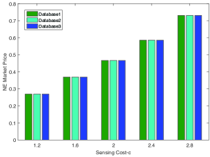
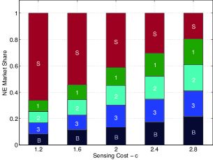
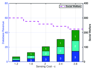
Figure 6: (a) Price equilibrium, (b) Market share equilibrium, (c) The system performance vs WSDs’ sensing cost

Figure 5.c shows each database’s revenue and the total social welfare (i.e., the total revenue of all databases plus the total payoffs of WSDs) achieved at the NE, under different values of network externality impact $\gamma$. Each bar denotes the aggregated revenue of $3$ databases, while each sub-bar corresponds to the revenue of a particular database $m$. The dash red line denotes the value of social welfare. The left y-axis denotes the value of database’s revenue, and the right y-axis denotes the value of social welfare. We can see that the databases’ aggregated revenue increases with the network externality level. This is because when the level of positive network externality increases, high utility provided by the advanced service drives the equilibrium prices as well as the equilibrium market shares up for all databases. The social welfare also increases with the network externality level. As the high level of positive network externality increases the quality of databases’ service, more WSDs choose to use the advanced service, which is cheaper than the sensing. Overall, this improves the social welfare.

VI-C Performance vs Sensing Cost

Figure 6 illustrates (a) price equilibrium, (b) market share equilibrium, and (c) system performance achieved under different sensing cost $c$ (from $1.2$ to $2.8$). In this simulation, we fix the network externality impact $\gamma_{1}=\gamma_{2}=\gamma_{3}=\gamma=0.4$, the number of database $M=3$, and the database’s operation cost as $c_{m}=0$, $m\in\mathcal{M}$.

Figure 6.a shows the price equilibrium under different values of sensing cost. We can see that the equilibrium market prices of databases increase with the sensing cost, as a higher sensing cost allows databases to increases their prices without losing WSDs.

Figure 6.b shows the equilibrium market shares achieved under different values of sensing cost. Each bar denotes the market share allocation among the basic service (denoted as “B”), database $m$’s advanced services (denoted as “$m$”), and sensing (denoted as “S”). As the sensing cost increases, the sensing services becomes less attractive, and hence the market share of sensing decreases with the sensing cost. Meanwhile, the market shares of basic service and all databases’ advanced services increase with the sensing cost.

Figure 6.c shows each database’s revenue and the total social welfare (i.e., the total revenue of all databases plus the total payoffs of WSDs) achieved at the NE, under different values of sensing cost $c$. Each bar denotes the aggregated revenue of $3$ databases, while each sub-bar corresponds to the revenue of database $m$. The dash red line denotes the value of social welfare. The left y-axis denotes the value of database’s revenue, and the right y-axis denotes the value of social welfare.

From Figure 6.c, we can see that the databases’ aggregated revenue increases with the sensing cost, as the advanced services become more attractive to the WSDs. However, as the sensing cost increasing, WSDs need to pay a higher price to enjoy a good quality of service, hence the social welfare decreases with sensing cost.

VI-D Performance vs Operational Cost of Database

Figure 7 illustrates (a) the price equilibrium, (b) the market share equilibrium, and (c) the system performance achieved under different operational costs of databases. In this simulation, we consider a scenario of $M=3$ databases with the same operational cost, i.e., $c_{1}=c_{2}=c_{3}$, and change such an operational cost from 0 to 0.2. Moreover, we fix the network externality factor $\gamma_{1}=\gamma_{2}=\gamma_{3}=0.4$ and the sensing cost $c=2$, and select slightly different initial market shares for three databases (i.e., $\eta_{3}>\eta_{2}>\eta_{1}$). In Figure 7.b, each bar with “S” or “B” denotes the percentage of WSDs choosing the sensing service or basic service, respectively, and each bar with number $m\in\{1,2,3\}$ denotes the percentage of WSDs choosing database $m$’s advanced service. In Figure 7.c, each bar with number $m\in\{1,2,3\}$ denotes the database $m$’s profit.

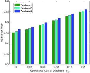
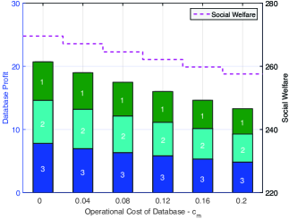
Figure 7: (a) Price equilibrium, (b) Market share equilibrium, (c) the system performance vs operational cost of database.

Figure 7.a shows the equilibrium market prices of databases under different operational costs. We can see that the equilibrium market prices of all databases increase with the operational cost. This is quite intuitive, as a higher operational cost drives the database to set a higher retail price in order to cover his operational cost.

Figure 7.b shows the equilibrium market shares achieved under different operational costs. Each bar denotes the market share allocation among the basic service (denoted as “B”), database $m$’s advanced services (denoted as “$m$”), and sensing (denoted as “S”). We have shown in Figure 7.a that with the increasing of database operational cost, all databases will set higher equilibrium market prices to cover their operational costs. This makes the advanced services become less attractive, and hence reduces the total market share of databases as shown in Figure 7.b. Accordingly, the market shares of both basic service and sensing service increase.

Figure 7.c shows the databases’ profits and the total social welfare (i.e., the total profit of all databases plus the total payoffs of WSDs) achieved at the market equilibrium, under different operational costs. Each bar denotes the aggregated profit of $3$ databases, while each sub-bar corresponds to the profit of database $m$. The dash red line denotes the value of social welfare. The left y-axis denotes the value of database’s profit, and the right y-axis denotes the value of social welfare. From Figure 7.c, we can see that both the databases’ aggregated profit and the social welfare decrease with the operational cost.

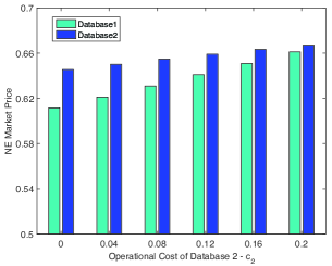
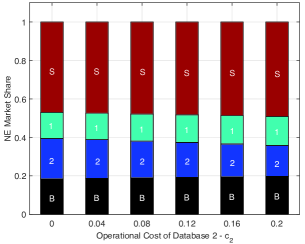
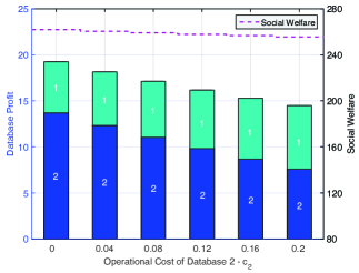
Figure 8: (a) Price equilibrium, (b) Market share equilibrium, and (c) the system performance vs the operational cost of database $2$.

We further consider the scenario of different operational costs for databases. To illustrate the results clearly, we consider a simple scenario of two databases with different operational costs. Specifically, we fix the operational cost of database 1 as $c_{1}=0.2$, while change the operational cost $c_{2}$ of database 2 from 0 to 0.2. The other parameters are same as those in the previous simulation. Figure 8 illustrates (a) the price equilibrium, (b) the market share equilibrium, and (c) the system performance, achieved under different operational costs of database 2.

Figure 8.a shows the price equilibrium under different operational costs of database 2. We can see with the increasing of operational cost $c_{2}$, database 2 will select a higher equilibrium market price in order to cover its operational cost; accordingly, database 1 can also set a higher equilibrium market price to gain more profit, even thought its own operational cost remains unchanged. We can also see that the price difference between two databases decreases with $c_{2}$, due to the decrease of their operation cost difference.

Figure 8.b shows the equilibrium market shares achieved under different operational costs of database 2. Each bar denotes the market share allocation among the basic service (denoted as “B”), database $m$’s advanced services (denoted as “$m$”), and sensing (denoted as “S”). We have shown in Figure 8.a that with the increase of the database $2$’s operational cost, both databases will set higher equilibrium market prices. This makes the advanced services of both databases becomes less attractive, and hence reduces the market share of databases and increases the the market shares of sensing service and basic service. Moreover, the market share of database 2 decreases, while that of database 1 slightly increases. This is because an increased operational cost of database 2 reduces its competitiveness, hence drives some of its market share to database 1.

Figure 8.c shows the databases’ profits and the total social welfare achieved at the market equilibrium, under different operational costs of database $2$. Each bar denotes the aggregated profit of $2$ databases, while each sub-bar corresponds to the profit of database $m$. The dash red line denotes the value of social welfare. The left y-axis denotes the value of database’s profit, and the right y-axis denotes the value of social welfare. From Figure 8.c, we can see that both the databases’ aggregated profit and the social welfare decrease with the operational cost. Moreover, the profit of database 2 decreases due to the reduction of its market share, while that of database 1 slightly increases due to the slight increase of its market share.

VII Conclusion

In this paper, we propose an information market model called MINE GOLD, which enables the geo-location databases to sell information regarding the white space to WSDs. We characterize the positive network externality in the proposed information market model, and study the user subscription dynamics and the associated market equilibrium. Based on this, we further examine the databases’ pricing decision from a game-theoretic perspective. We discover several interesting insights of the databases’ competition game in the information market. For example, there exists an optimal number of databases to achieve the maximum total database revenue. Moreover, a larger positive network externality will have a more positive impact on the system performance, both in terms of the databases’ revenues and the social welfare.

The information market proposed in this paper mainly concerns the utilization of unlicensed TV channels, where WSDs share with others. In practice, some licensees are willing to lease their under-utilized licensed spectrum for extra profit, and WSDs can have exclusive usage right by leasing such spectrum. Hence, a joint market design involving both unlicensed and licensed TV channels will be an important future research direction.

Appendix A Appendix

A-A Property of Information Market

In this section, we will discuss the properties of positive network externality in the information market. For illustration purpose, we first define the advanced information as the interference level on each channel, then we characterize the information value to the WSDs, based on which we can further characterize the properties of the information market.

A-A1 Interference Information

For each WSD $n\in\mathcal{N}$ operating on the TV channel, each channel $k$ is associated with an interference level, denoted by $Z_{n,k}$, which reflects the aggregate interference from all other nearby devices (including TV stations and other WSDs) operating on this channel. Due to the fast changing of wireless channels and the uncertainty of WSDs’ mobilities and activities, the interference $Z_{n,k}$ is a random variable. We impose assumptions on the interference $Z_{n,k}$ as follows.

Assumption 5.

For each WSD $n\in\mathcal{N}$, each channel $k$’s interference level $Z_{n,k}$ is temporal-independence and frequency-independence.

This assumption shows that (i) the interference $Z_{n,k}$ on channel $k$ is independent identically distributed (iid) at different times, and (ii) the interferences on different channels, $Z_{n,k},k\in\mathcal{K}$, are also iid at the same time. As we are talking about a general WSD $n$, we will omit the WSD index $n$ in the notations (e.g., write $Z_{n,k}$ as $Z_{k}$), whenever there is no confusion caused. Let $H_{Z}(\cdot)$ and $h_{Z}(\cdot)$ denote the cumulative distribution function (CDF) and probability distribution function (PDF) of $Z_{k}$, $\forall k\in\mathcal{K}$.

Usually, a particular WSD’s experienced interference $Z_{k}$ on a channel $k$ consistss of the following three components:

1. $U_{k}$: the interference from licensed TV stations;

2. $W_{k,j}$: the interference from another WSD $j$ operating on the same channel $k$;

3. $V_{k}$: any other interference from outside systems.

The total interference on channel $k$ is $Z_{k}=U_{k}+W_{k}+V_{k}$, where $W_{k}\triangleq\sum_{j\in\mathcal{N}_{k}}W_{k,j}$ is the total interference from all other WSDs operating on channel $k$ (denoted by $\mathcal{N}_{k}$). Similar to $Z_{k}$, we also assume that $U_{k},W_{k},W_{k,j}$, and $V_{k}$ are random variables with temporal-independence (i.e., iid across time) and frequency-independence (i.e., iid across frequency). We further assume that $W_{k,j}$ is user-independence, i.e., $W_{k,j},j\in\mathcal{N}_{k}$, are iid. It is important to note that different WSDs may experience different interferences $U_{k}$ (from TV stations), $W_{k,j}$ (from another WSD operating on the same channel), and $V_{k}$ (from outside systems) on a channel $k$, as we have omitted the WSD index $n$ for all these notations for clarity.

Next we discuss these interferences in more details.

• Each database is able to compute the interference $U_{k}$ from TV stations to every WSD (on channel $k$), as it knows the locations and channel occupancies of all TV stations.

• Each database cannot compute the interference $V_{k}$ from outside systems, due to the lack of outside interference source information. Thus, the interference $V_{k}$ will not be included in a database’s advanced information sold to WSDs.

• Each database may or may not be able to compute the interference $W_{k,j}$ from another WSD $j$, depending on whether WSD $j$ subscribes to the database’s advanced service. Specifically, if WSD $j$ subscribes to the advanced service, the database can predict its channel selection (since the WSD is fully rational and will always choose the channel with the lowest interference level indicated by the database at the time of subscription), and thus can compute its interference to any other WSD. However, if WSD $j$ only chooses the database’s basic service, the database cannot predict its channel selection, and thus cannot compute its interference to other WSDs.

For convenience, we denote $\mathcal{N}_{k}^{[m]},m\in\mathcal{M}$, as the set of WSDs operating on channel $k$ and subscribing to the database $m$’s advance service (i.e., those choosing the strategy $l=m$), $\mathcal{N}_{k}^{[\textsf{b}]}$ as the set of WSDs operating on channel $k$ and choosing the database’s basic service (i.e., those choosing the strategy $l=\textsf{b}$), and $\mathcal{N}_{k}^{[\textsf{s}]}$ as the set of WSDs operating on channel $k$ and sensing all the available channels (i.e., those choosing the strategy $l=\textsf{s}$). That is, $\bigcup_{m\in\mathcal{M}}\mathcal{N}_{k}^{[m]}\bigcup\mathcal{N}_{k}^{[\textsf{b}]}\bigcup\mathcal{N}_{k}^{[\textsf{s}]}=\mathcal{N}_{k}$. Then, for a particular WSD, its experienced interference (on channel $k$) known by database $m$ is

$$\textstyle X^{m}_{k}\triangleq U_{k}+\sum_{j\in\mathcal{N}_{k}^{[m]}}W_{k,j},$$ (29)

which contains the interference from TV licensees and all WSDs (operating on channel $k$) subscribing to the database$m$’s advanced service. The WSD’s experienced interference (on channel $k$) not known by the database $m$ is

$$\textstyle Y^{m}_{k}\triangleq V_{k}+\sum_{j\in\mathcal{N}_{k}^{[\textsf{b}]}}W_{k,j}$$ (30)

$$+\sum_{j\in\mathcal{N}_{k}^{[\textsf{s}]}}W_{k,j}+\sum_{j\in\mathcal{N}_{k}^{[i]},i\neq m}W_{k,j},$$

which contains the interference from outside systems and all WSDs (operating on channel $k$) not subscribing to the database $m$’s advanced service. Obviously, both $Y^{m}_{k}$ and $X^{m}_{k}$ are also random variables with temporal- and frequency-independence. Accordingly, the total interference on channel $k$ for a WSD can be written as $\textstyle Z_{k}=X^{m}_{k}+Y^{m}_{k}.$

Since the database $m$ knows only $X^{m}_{k}$, it will provide this information (instead of the total interference $Z_{k}$) as the advanced service to a subscribing WSD. It is easy to see that the more WSDs subscribing to the database $m$’s advanced service, the more information the database $m$ knows, and the more accurate the database $m$’s information will be.

Next we can characterize the accuracy of a database’s information explicitly. Note that $\eta_{{m}}$ and $\eta_{s}$ denote the fraction of WSDs choosing the database $m$’s advanced service and sensing service, respectively. Moreover, $(1-\sum_{m\in\mathcal{M}}\eta_{{m}}-\eta_{s})$ denotes the fraction of WSDs choosing the basic service. Due to the Assumption 5, it is reasonable to assume that each channel $k\in\mathcal{K}$ will be occupied by an average of $\frac{N}{K}$ WSDs. Then, among all $\frac{N}{K}$ WSDs operating on channel $k$, there are, on average, $\frac{N}{K}\cdot\eta_{{m}}$ WSDs subscribing to the database $m$’s advanced service, $\frac{N}{K}\cdot\eta_{s}$ WSDs choosing sensing service, and $\frac{N}{K}\cdot(1-\sum_{m\in\mathcal{M}}\eta_{{m}}-\eta_{s})$ WSDs choosing the basic service. That is, $|\mathcal{N}_{k}|=\frac{N}{K}$, $|\mathcal{N}_{k}^{[m]}|=\frac{N}{K}\cdot\eta_{{m}}$, $|\mathcal{N}_{k}^{[\textsf{s}]}|=\frac{N}{K}\cdot\eta_{s}$, and $|\mathcal{N}_{k}^{[\textsf{b}]}|=\frac{N}{K}\cdot(1-\sum_{m\in\mathcal{M}}\eta_{{m}}-\eta_{s})$. Finally, by the user-independence of $W_{k,m}$, we can immediately calculate the distributions of $X^{m}_{k}$ and $Y^{m}_{k}$ under any given market share $\eta_{{m}}$ $m\in\mathcal{M}$ via (29) and (30).

A-A2 Information Value

Now we evaluate the value of the database $m$’s advanced information to WSDs, which is reflected by the WSD’s benefit (utility) that can be achieved from this information.

We first consider the expected utility of a WSD when choosing the database’s basic service (i.e., $l=\textsf{b}$). In this case, the WSD will randomly choosing a TV channel based on the information provided in the free basic service, and its expected data rate is

$$\textstyle R_{[\textsf{b}]}\textstyle=\mathrm{E}_{Z}[\mathcal{R}(Z)]=\int_{z}\mathcal{R}(z)\mathrm{d}H_{Z}(z),$$ (31)

where $\mathcal{R}(\cdot)$ is the transmission rate function (e.g., the Shannon capacity) under any given interference. As shown in Section A-A1, each channel $k\in\mathcal{K}$ will be occupied by an average of $\frac{N}{K}$ WSDs based on the Assumption 5. Hence, $R_{[\textsf{b}]}$ depends only on the distribution of the total interference $Z_{k}$, while not on the specific distributions of $X^{m}_{k}$ and $Y^{m}_{k}$. Then the expected utility provided by the basic service is:

$$\textstyle B=\textstyle U\big{(}R_{[\textsf{b}]}\big{)},$$ (32)

where $U(\cdot)$ is the utility function of the WSD. We can easily check that the accuracy of the database $m$’s information does not affect the utilities of theses WSDs not subscribing to the database $m$’s advanced service.

Then we consider the expected utility of a WSD when choosing the sensing service (i.e., $l=\textsf{s}$). In this case, the WSD will sense all the available channels and select one with the lowest interference level. Hence, its expected data rate is

$$\textstyle R_{[\textsf{s}]}\textstyle=\mathrm{E}_{Z_{(1)}}[\mathcal{R}(Z)]=\int_{z}\mathcal{R}(z)\mathrm{d}H_{Z_{(1)}}(z),$$ (33)

where $Z_{(1)}\triangleq\min\{Z_{1},...,Z_{K}\}$ denotes the minimum interference on all channels, $H_{Z_{(1)}}(z)=[1-H_{Z}(z)]^{K}$ is the CDF of $Z_{(1)}$, and $\mathcal{R}(\cdot)$ is the transmission rate function (e.g., the Shannon capacity). We can check that $R_{[\textsf{s}]}$ depends only on the distribution of the total interference $Z_{k}$, while not on the specific distributions of $X^{m}_{k}$ and $Y^{m}_{k}$. Then the expected utility provided by the sensing service is:

$$\textstyle S=\textstyle U\big{(}R_{[\textsf{s}]}\big{)},$$ (34)

where $U(\cdot)$ is the utility function of the WSD. We can easily check that the accuracy of the database $m$’s information does not affect the utilities of theses WSDs not subscribing to the database $m$’s advanced service. We, therefore, have the Assumption 1.

Then we consider the expected utility of a WSD when subscribing to the database $m$’s advance service (i.e., $l=m,m\in\mathcal{M}$). In this case, the database $m$ returns the interference $\{X^{m}_{k}\}_{k\in\mathcal{K}}$ to the WSD subscribing to the advanced service, together with the basic information such as the available channel list. For a rational WSD, it will always choose the channel with the minimum $X^{m}_{k}$ (since $\{Y^{m}_{k}\}_{k\in\mathcal{K}}$ are iid). Let $X_{(1)}^{[m]}=\min\{X^{m}_{1},\ldots,X^{m}_{K}\}$ denote the minimum interference indicated by the database $m$’s advanced information. Then, the actual interference experienced by a WSD (subscribing to the database $m$’s advanced service) can be formulated as the sum of two random variables, denoted by $Z_{[\textsf{a}]}^{m}=X_{(1)}^{m}+Y^{m}$. Accordingly, the WSD’s expected data rate under the strategy $l=m$ can be computed by

$$R_{\textsf{a}}^{m}(\eta_{{m}}) \textstyle=\mathrm{E}_{Z_{[\textsf{a}]}^{m}}\big{[}\mathcal{R}\left(Z_{[\textsf{a}]}^{m}\right)\big{]}=\int_{z}\mathcal{R}(z)\mathrm{d}H_{Z_{[\textsf{a}]}^{m}}(z),$$ (35)

where $H_{Z_{[\textsf{a}]}^{m}}(z)$ is the CDF of $Z_{[\textsf{a}]}^{m}$. It is easy to see that $R_{\textsf{a}}^{m}$ depends on the distributions of $X^{m}_{k}$ and $Y^{m}_{k}$, and thus depend on the market share $\eta_{{m}}$. Thus, we will write $R_{\textsf{a}}^{m}$ as $R_{\textsf{a}}^{m}(\eta_{{m}})$. Accordingly, the advanced service’s utility is:

$$A^{m}(\eta_{{m}}) \textstyle\triangleq U\bigg{(}R_{\textsf{a}}^{m}(\eta_{{m}})\bigg{)}$$ (36)

By further checking the properties of $B$, $S$, and $A^{m}(\eta_{{m}})$, we have the Assumption 2-4.

A-B Proof for Lemma 1

Proof.

By solving (3), we can get three thresholds, denoted by

$$\textstyle\theta_{\textsc{SB}}^{t}\triangleq\frac{c}{S-B},~{}~{}~{}~{}\theta_{\textsc{AB}}^{t}\triangleq\frac{\pi_{1}}{A_{1}(\eta_{{1}}^{t})-B},~{}~{}~{}~{}\theta_{\textsc{SA}}^{t}\triangleq\frac{c-\pi_{1}}{S-A_{1}(\eta_{{1}}^{t})}.$$

Consider two cases: (i) $\theta_{\textsc{SB}}^{t}>\theta_{\textsc{AB}}^{t}$, and (ii) $\theta_{\textsc{SB}}^{t}\leq\theta_{\textsc{AB}}^{t}$.

(i) When $\theta_{\textsc{SB}}^{t}>\theta_{\textsc{AB}}^{t}$, it is easy to check that

$$\theta_{\textsc{SA}}^{t}-\theta_{\textsc{SB}}^{t}=\frac{c\cdot\big{(}A_{1}(\eta_{{1}}^{t})-B\big{)}-\pi_{1}\cdot(S-B)}{\big{(}S-A_{1}(\eta_{{1}}^{t})\big{)}\cdot(S-B)}>0,$$

since $S>A_{1}\big{(}\eta_{{1}}^{t}\big{)}$, $S>B$, and $c\cdot(A_{1}(\eta_{{1}}^{t})-B)>\pi_{1}\cdot(S-B)$ as $\theta_{\textsc{SB}}^{t}>\theta_{\textsc{AB}}^{t}$. Hence, we have: $\theta_{\textsc{SA}}^{t}>\theta_{\textsc{SB}}^{t}>\theta_{\textsc{AB}}^{t}$. Accordingly, the newly derived market share is:

$$\eta_{{1}}^{t}=\theta_{\textsc{SA}}^{t}-\theta_{\textsc{AB}}^{t},$$

(ii) When $\theta_{\textsc{SB}}^{t}\leq\theta_{\textsc{AB}}^{t}$, we can similarly check that $\theta_{\textsc{SA}}^{t}-\theta_{\textsc{SB}}^{t}<0$, and hence $\theta_{\textsc{SA}}^{t}<\theta_{\textsc{SB}}^{t}<\theta_{\textsc{AB}}^{t}.$ Accordingly, the newly derived market share $\eta_{{1}}^{t}$ is

$$\eta_{{1}}^{t}=0.$$

Formally, based on the above (i) and (ii), we can get the result in (4). ∎

A-C Proof for Proposition 1

Proof.

By Definition 1, $\eta_{{1}}^{*}$ is an equilibrium point, if and only if it is a solution of (6). We consider two cases: (i) $\theta_{\textsc{SB}}>\theta_{\textsc{AB}}$ and (ii) $\theta_{\textsc{SB}}\leq\theta_{\textsc{AB}}$.

(i) If $\theta_{\textsc{SB}}>\theta_{\textsc{AB}}$, the solution $\eta_{{1}}$ should satisfy

$$\triangle\eta_{{1}}(\eta_{{1}})=\frac{c-\pi_{1}}{S-A_{1}(\eta_{{1}})}-\frac{\pi_{1}}{A_{1}(\eta_{{1}}^{t})-B}-\eta_{{1}}=0.$$ (37)

It is easy to check that $\left.\triangle\eta_{{1}}(\eta_{{1}})\right|_{\eta_{{1}}=0}>0$ and $\left.\triangle\eta_{{1}}(\eta_{{1}})\right|_{\eta_{{1}}=1}<0$. As $\triangle\eta_{{1}}(\eta_{{1}})$ is continuous on $[0,1]$, we have: $\triangle\eta_{{1}}(\eta_{{1}})=0$ has at least one root on $[0,1]$.

(ii) If $\theta_{\textsc{SB}}\leq\theta_{\textsc{AB}}$, the solution $\eta_{{1}}^{*}=0$ directly. ∎

A-D Proof for Proposition 2

Proof.

To prove the uniqueness, we need to show that the function $\triangle\eta_{{1}}(\eta_{{1}})$ in (37) is strictly decreasing on $[0,1]$. First, we can easily check that if

$$g^{\prime}(\eta_{{1}})\cdot\left[\frac{c-\pi_{1}}{(S-A_{1}(\eta_{{1}}))^{2}}+\frac{\pi_{1}}{(A_{1}(\eta_{{1}})-B)^{2}}\right]<1,$$ (38)

then the first derivative of $\triangle\eta_{{1}}(\eta_{{1}})$ is negative, hence $\triangle\eta_{{1}}(\eta_{{1}})$ in (37) is strictly decreasing on $[0,1]$.

We further notice that $\frac{c-\pi_{1}}{(S-A_{1}(\eta_{{1}}))}\leq 1$ and $\frac{\pi_{1}}{A_{1}(\eta_{{1}})-B}\leq 1$, and

$$g^{\prime}(\eta_{{1}})\cdot\left[\frac{c-\pi_{1}}{(S-A_{1}(\eta_{{1}}))^{2}}+\frac{\pi_{1}}{(A_{1}(\eta_{{1}})-B)^{2}}\right]$$ (39)

$$\leq\max\bigg{\{}\frac{c-\pi_{1}}{(S-A_{1}(\eta_{{1}}))},\frac{\pi_{1}}{(A_{1}(\eta_{{1}})-B)}\bigg{\}}\cdot\frac{A_{1}^{\prime}(\eta_{{1}})}{A_{1}(\eta_{{1}})-B}\cdot\frac{S-B}{S-A_{1}(\eta_{{1}})}.$$

Hence, the condition in (38) is satisfied when

$$\max_{\eta_{{1}}\in[0,1]}\frac{A_{1}^{\prime}(\eta_{{1}})}{A_{1}(\eta_{{1}})-B}\cdot\frac{S-B}{S-A_{1}(\eta_{{1}})}\leq 1,$$ (40)

∎

A-E Proof for Theorem 1

Proof.

By Propositions 1 and 2, together with the non-decreasing of $g(\cdot)$, we can get the conclusion. ∎

A-F Proof for Proposition 3

Proof.

By Proposition 2, there exist an one-to-one mapping between the information price and market share. Hence, we can get the conclusion immediately. ∎

A-G Proof for Proposition 4

Proof.

The proof for the existence is straightforward. Next we show there exists an unique optimal price under both the low sensing cost region and high sensing cost region.

We first look at the database’s revenue under high sensing cost region: $\Pi^{\textsc{db}}_{1}(\eta_{{1}})=(\pi_{1}-c_{1})\cdot\eta_{{1}}(\pi_{1})$, where $\eta_{{1}}(\pi_{1})$ is given by

$$1-\frac{\pi_{1}}{A(\eta_{{1}})-B}-\eta_{{1}}=0.$$

The second order derivative of $\Pi^{\textsc{db}}_{1}(\pi)$ with respect to $\pi_{1}$ is

$$\frac{\partial^{2}{\Pi^{\textsc{db}}_{1}}}{\partial{\pi_{1}^{2}}}=2\cdot\frac{\mathrm{d}\eta_{{1}}}{\mathrm{d}\pi_{1}}+(\pi_{1}-c_{1})\cdot\frac{\mathrm{d^{2}}\eta_{{1}}}{\mathrm{d}\pi_{1}^{2}}.$$

It is easily to verify that

$$\frac{\mathrm{d^{2}}\eta_{{1}}}{\mathrm{d}\pi_{1}^{2}}=-\pi_{1}\cdot\frac{[A_{1}(\eta_{{1}})-B]A_{1}^{\prime}(\eta_{{1}})}{[\pi_{1}A_{1}^{\prime}(\eta_{{1}})-(A_{1}(\eta_{{1}})-B)^{2}]^{4}}\leq 0.$$

where $A_{1}^{\prime}(\eta_{{1}})={\mathrm{d}A_{1}(\eta_{{1}})}/{\mathrm{d}\pi_{1}}>0$. Moreover, $\eta_{{1}}(\pi_{1})$ decreases with $\pi_{1}$. Therefore, we have $\frac{\partial^{2}{\Pi^{\textsc{db}}_{1}}}{\partial{\pi_{1}^{2}}}<0$, and thus there exist a unique solution that maximizes $\Pi^{\textsc{db}}_{1}(\pi_{1})$.

Similarly, we can prove that under the high price region, there exists an unique solution that maximizes $\Pi^{\textsc{db}}_{1}(\pi_{1})$. ∎

A-H Proof for Proposition 2

Proof.

Given market shares $\{\eta_{{1}}^{t},\eta_{{2}}^{t},\ldots,\eta_{{M}}^{t}\}$ in slot $t$ with $\eta_{{M}}^{t}>\eta_{{M-1}}^{t}>\ldots>\eta_{{1}}^{t}$, we have: $S>A_{M}(\eta_{{M}}^{t})>A_{M-1}(\eta_{{M-1}}^{t})>\ldots>A_{1}(\eta_{{1}}^{t})$. Notice that no WSD is willing to choose a service with a lower QoS and a higher price. Hence, we can focus on the non-trivial scenario with $c>\pi_{M}>\pi_{M-1}>\ldots>\pi_{1}$, under which we can get the conclusion immediately by solving (16) - (18). ∎

A-I Proof for Theorem 2

Proof.

By Definition 2 , $\boldsymbol{\eta}^{*}$ is an equilibrium point, if and only if it it a solution of (21). Given market shares $\{\eta_{{1}}^{t},\eta_{{2}}^{t},\ldots,\eta_{{M}}^{t}\}$ in slot $t$ with $\eta_{{M}}^{t}>\eta_{{M-1}}^{t}>\ldots>\eta_{{1}}^{t}$, the solution $\boldsymbol{\eta}$ should satisfy

$$\left\{\begin{aligned} &\frac{c-\pi_{M}}{S-A_{M}(\eta_{{M}})}-\frac{\pi_{M}-\pi_{M-1}}{A_{M}(\eta_{M})-A_{M-1}(\eta_{M-1})}-\eta_{{M}}=0,\\ &\frac{\pi_{m+1}-\pi_{m}}{A_{m+1}(\eta_{m+1})-A_{m}(\eta_{m})}-\frac{\pi_{m}-\pi_{m-1}}{A_{m}(\eta_{m})-A_{m-1}(\eta_{m-1})}-\eta_{{m}}=0,\ \forall m=2,\ldots,M-1,\\ &\frac{\pi_{2}-\pi_{1}}{A_{2}(\eta_{2})-A_{1}(\eta_{1})}-\frac{\pi_{1}}{A_{1}(\eta_{{1}})-B}-\eta_{{1}}=0.\end{aligned}\right.$$ (41)

By solving the above equation, we can get the conclusion immediately. ∎

A-J Proof for Proposition 5

Proof.

We first notice that the best response dynamics must converge to a market share equilibrium, as the changing of each database’s market share is monotonic. This is due to the positive externality of information market, under which a database with an increased market share in a slot tends to get more market share in the future.

Next, we can easily find that given a particular market share set in a slot, the best response dynamics will evolve to a fixed newly derived market share set in the next slot, and eventually converge to a unique market share equilibrium. ∎

A-K Proof for Proposition 6

Proof.

If $\boldsymbol{\eta}_{\textsc{a}}^{*}$ is a Nash equilibrium of MSCG, then we have:

$$\eta_{{m}}^{*}=\arg\max_{\eta_{{m}}}\widetilde{\Pi}^{\textsc{db}}_{m}(\eta_{{m}},\boldsymbol{\eta}_{-m}^{*})$$ (42)

By (25), we further have:

$$\textstyle\pi_{m}=\sum_{m=1}^{M+1}\left[\left(1-\sum_{n=m}^{M+1}\eta_{n}\right)\cdot(g(\eta_{m})-g(\eta_{m-1}))\right]$$ (43)

Hence, we can easily check that $\boldsymbol{\pi}^{*}$ is a Nash equilibrium of PCG, where

$$\pi_{m}^{*}=\arg\max_{\pi_{m}\geq 0}\ \Pi^{\textsc{db}}_{m}(\pi_{m},\boldsymbol{\pi}_{-m}^{*}),~{}~{}\forall m\in\mathcal{M}.$$ (44)

∎

A-L Proof for Lemma 3

Proof.

For convenience, we first give the formal definition of supermodular game and some related important concepts [21]. A real $n-$diensional set $\mathcal{V}$ is a sublattice of $\mathbb{R}^{n}$ if for any two elements $a,b\in\mathcal{V}$, the component-wise minimum, $a\vee b$, and the component-wise maximum, $a\wedge b$, are also in $\mathcal{V}$. Particularly, a compact sublattice has a smallest and largest element. A function $f(x_{1},\ldots,f_{N})$ has increasing differences in $(x_{i},x_{j})$ for all $i\neq j$ if $f(x_{1},\ldots,x^{1}_{i},\ldots,x_{N})-f(x_{1},\ldots,x^{2}_{i},\ldots,x_{N})$ is increasing in $x_{j}$ for all $x^{2}_{i}-x^{1}_{i}>0$. The formal definition of a supermodular game is given below:

Definition 4 (Supermodular Game [21]).

A noncooperative game $(\mathcal{M},\{S\}_{m\in\mathcal{M}},\{U_{m}\}_{m\in\mathcal{M}})$ is called a supermodular game if the following conditions are all satisfied:

• The strategy set ${S_{m}}$ is a nonempty and compact sublattice of real number.

• The payoff function $U_{m}$ is supermodular in player $m$’s own strategy.

• The payoff function $U_{m}$ has increasing differences in all sets of strategies.

To prove the existence of equilibrium under duopoly scenario, we only need to prove that the MSCG is a supermodular game under duopoly scenario with respect to $\eta_{1}$ and $-\eta_{2}$. Since the two databases with a single instrument $\boldsymbol{\eta}=(\eta_{1},\eta_{2})$ chosen from a compact set $[0,1]^{2}$, it suffices to show that both $\widetilde{\Pi}^{\textsc{db}}_{1}(\eta_{1},-\eta_{2})$ and $\widetilde{\Pi}^{\textsc{db}}_{2}(\eta_{1},-\eta_{2})$ have increasing difference in $(\eta_{1},\eta_{2})$. By (25) and (26), we have:

$$\frac{\partial^{2}{\widetilde{\Pi}^{\textsc{db}}_{1}(\eta_{1},-\eta_{2})}}{\partial{({\eta_{1}})}\partial{-\eta_{2}}}=\frac{\mathrm{d}{A_{1}}}{\mathrm{d}{\eta_{1}}}\cdot\eta_{1}+(A_{2}-B)\geq 0$$ (45)

$$\frac{\partial^{2}{\widetilde{\Pi}^{\textsc{db}}_{2}(\eta_{1},-\eta_{2})}}{\partial{({\eta_{1}})}\partial{-\eta_{2}}}=A_{1}-B\geq 0{}{}{}{}{}{}{}{}{}{}{}{}{}{}{}{}$$ (46)

Hence, we can conclude that MSCG is a supermodular game with respect to $\eta_{1}$ and $-\eta_{2}$. ∎

A-M Proof for Proposition 7

Proof.

To prove the existence of equilibrium under oligopoly scenario, we only need to prove that $\widetilde{\Pi}^{\textsc{db}}_{m}(\eta_{{m}},\boldsymbol{\eta}_{-m})$, $\forall m\in\mathcal{M}$, is quasi-concave in $\eta_{{m}}$ [22].

To prove $\widetilde{\Pi}^{\textsc{db}}_{m}(\eta_{{m}},\boldsymbol{\eta}_{-m})$ is quasi-concave in $\eta_{{m}}$, it is sufficient to show that $\frac{\partial{\widetilde{\Pi}^{\textsc{db}}_{m}(\eta_{{m}},\boldsymbol{\eta}_{-m})}}{\partial{\eta_{{m}}}}$ changes the sign once. We first notice that $\eta_{{m}}$ is chosen from $[0,1]$, and

$$\lim_{\eta_{{m}}\rightarrow 0}\frac{\partial{\widetilde{\Pi}^{\textsc{db}}_{m}(\eta_{{m}},\boldsymbol{\eta}_{-m})}}{\partial{\eta_{{m}}}}>0,\mbox{~{}and~{}}\lim_{\eta_{{m}}\rightarrow+1}\frac{\partial{\widetilde{\Pi}^{\textsc{db}}_{m}(\eta_{{m}},\boldsymbol{\eta}_{-m})}}{\partial{\eta_{{m}}}}<0.$$ (47)

Then we consider the second order derivative of $\widetilde{\Pi}^{\textsc{db}}_{m}(\eta_{{m}},\boldsymbol{\eta}_{-m})$ with respect to $\eta_{{m}}$. We have:

$$\frac{\partial^{2}{\widetilde{\Pi}^{\textsc{db}}_{m}(\eta_{{m}})}}{\partial{\eta_{{m}}^{2}}} =-(\gamma_{m}^{2}+3\gamma_{m}+1)\cdot\eta_{{m}}+\gamma_{m}\cdot(\gamma_{m}+1)\cdot\bigg{(}1-\sum_{h=m+1}^{M}\eta_{h}\bigg{)},$$ (48)

which is a linear function of $\eta_{{m}}$. We can further check that

$$\lim_{\eta_{{m}}\rightarrow 0}\frac{\partial^{2}{\widetilde{\Pi}^{\textsc{db}}_{m}(\eta_{{m}},\boldsymbol{\eta}_{-m})}}{\partial{\eta_{{m}}^{2}}}>0,\mbox{~{}and~{}}\lim_{\eta_{{m}}\rightarrow+1}\frac{\partial^{2}{\widetilde{\Pi}^{\textsc{db}}_{m}(\eta_{{m}},\boldsymbol{\eta}_{-m})}}{\partial{\eta_{{m}}^{2}}}<0.$$

Hence, the second order derivative of $\frac{\partial^{2}{\widetilde{\Pi}^{\textsc{db}}_{m}(\eta_{{m}})}}{\partial{\eta_{{m}}^{2}}}$ is first positive when $\eta_{{m}}$ is less than a threshold, and then changes to negative when $\eta_{{m}}$ is larger than a threshold. This implies that the first order derivative ${\partial{\widetilde{\Pi}^{\textsc{db}}_{m}(\eta_{{m}},\boldsymbol{\eta}_{-m})}}/{\partial{\eta_{{m}}}}$ first increases (from a positive value), and then decreases to a negative value, hence it changes the sign only once. ∎

A-N Proof for Proposition 8

Proof.

To prove the uniqueness of NE, we only need to verify that:

$$-\frac{\partial^{2}{\widetilde{\Pi}^{\textsc{db}}_{m}(\eta_{{m}},\boldsymbol{\eta}_{-m})}}{\partial{(-{\eta_{{m}}})}^{2}}\geq\sum_{j\neq m}\frac{\partial^{2}{\widetilde{\Pi}^{\textsc{db}}_{m}(\eta_{{m}},\boldsymbol{\eta}_{-m})}}{\partial{{(-\eta_{{m}})}}\partial{\eta_{{n}}}},\quad\forall m\in\mathcal{M}.$$ (49)

The above condition is usually called the dominant diagonal condition. Hence, as long as $\widetilde{\Pi}^{\textsc{db}}_{m}(\eta_{{m}},\boldsymbol{\eta}_{-m})$ satisfy the above condition, the MSCG has a unique NE, so does the original PCG [21]. ∎

References

- [1] The Climate Group SMART 2020 Report, “SMART2020: Enabling the Low Carbon Economy in the Information Age”, http://www.theclimategroup.org, June, 2008.
- [2] FCC 12-36, Third Memorandum Opinion and Order, 2012.
- [3] Ofcom, “Implementing Geolocation”, Feb. 2015.
- [4] D. Niyato, E. Hossain, and Z. Han, “Dynamic Spectrum Access in IEEE 802.22-based Cognitive Wireless Networks: A Game Theoretic Model for Competitive Spectrum Bidding and Pricing”, IEEE Wireless Commun., vol. 16, no. 2, pp:16-23, 2009.
- [5] Y. Luo, L. Gao, and J. Huang, “Spectrum Broker by Geo-location Database”, IEEE GLOBECOM, 2012.
- [6] H. Bogucka, M. Parzy, P. Marques, J. W. Mwangoka, T. Forde, “Secondary Spectrum Trading in TV White Spaces”, IEEE Commun. Mag., vol. 50, no. 11, pp. 121-129, Nov. 2012.
- [7] X. Feng, J. Zhang, and J. Zhang, “Hybrid Pricing for TV White Space Database”, IEEE INFOCOM, 2013.
- [8] Y. Luo, L. Gao, and J. Huang, “White Space Ecosystem: A Secondary Network Operator’s Perspective”, IEEE GLOBECOM, 2013.
- [9] Y. Luo, L. Gao, and J. Huang, “Price and Inventory Competition in Oligopoly TV White Space Markets”, IEEE J. Sel. Areas Commun., vol. 33, no. 5, pp. 1002-1013, Oct. 2014.
- [10] Y. Luo, L. Gao, and J. Huang, “Trade Information, Not Spectrum: A Novel TV White Space Information Market Model”, IEEE WiOpt, 2014.
- [11] Y. Luo, L. Gao, and J. Huang, “Information Market for TV White Space”, IEEE INFOCOM Workshop on SDP, 2014.
- [12] Y. Luo, L. Gao, and J. Huang, “Business Modeling for TV White Space Networks”, IEEE Commun. Mag., vol. 53, no. 5, pp. 82-88, May 2015.
- [13] Y. Luo, L. Gao, and J. Huang, “HySIM: A Hybrid Spectrum and Information Market for TV White Space Networks”, IEEE INFOCOM, 2015.
- [14] D. Niyato and E. Hossain, “Competitive Pricing for Spectrum Sharing in Cognitive Radio Networks: Dynamic Game, Inefficiency of Nash Equilibrium, and Collusion,” IEEE J. Sel. Areas Commun., vol.26, no. 1, pp. 192-202, Jan. 2008.
- [15] G. S. Kasbekar and S. Sarkar, “Spectrum Pricing Games with Spatial Reuse in Cognitive Radio Networks,” IEEE J. Sel. Areas Commun., vol.30, no. 1, pp. 153-164, Jan. 2012.
- [16] N. Shetty, G. Schwartz, and J. Walrand, “Internet QoS and Regulations”, IEEE Trans. Networking, vol. 17, no. 6, pp. 1725-1737, Dec. 2010.
- [17] M. A. Khan, H. Tembine, and A. V. Vasilakos, “Game Dynamics and Cost of Learning in Heterogeneous 4G Networks”, IEEE J. Sel. Areas Commun., vol.30, no. 1, pp. 198-213, Jan. 2012.
- [18] J. Palicot, “Cognitive Radio: An Enabling Technology for the Green Radio Communications Concept”, ACM IWCMC, June. 2009.
- [19] G. Gr and F. Alagz, “Green Wireless Communications via Cognitive Dimension: An Overview”, IEEE Netw., vol. 25, no. 2, pp. 50-56, March-April. 2011.
- [20] Z. Ji, I. Ganchev, M, O’Droma, and X. Zhang, “A Realization of Broadcast Cognitive Pilot Channels Piggybacked on T-DMB”, Trans. Emerging Tel. Tech., vol. 24, no. 7-8, pp. 709-723, Dec. 2013.
- [21] D. M. Topkis, Supermodularity and Complementarity, Princeton Univ. Press, 1998.
- [22] D. Fudenberg and J. Tirole, Game Theory, MIT Press, 1991
- [23] D. Easley and J. Kleinberg, Networks, Crowds, and Markets, Cambridge Univeristy Press, Cambridge, 2010.
- [24] G. Gallego, W. T. Huh, W. Kang, and R. Phillips, “Price Competition with the Attraction Demand Model: Existence of Unique Equilibrium and Its Stability”, Manufacturing Service Oper. Manag., vol. 8, no. 4, pp. 359-375, 2006.
- [25] X. Vives, Oligopoly Pricing, MIT Press, Cambridge, 1991.
- [26] K. Jain, V. Bazirani, “Eisenberg-Gale Markets: Algorithms and Game-Theoretic Properties”, Game and Economics Behavior, vol. 70, no. 1, pp. 84-106, Sept. 2010.