Abstract

We propose a multiscale method for elliptic problems on complex domains, e.g. domains with cracks or complicated boundary. For local singularities this paper also offers a discrete alternative to enrichment techniques such as XFEM. We construct corrected coarse test and trail spaces which takes the fine scale features of the computational domain into account. The corrections only need to be computed in regions surrounding fine scale geometric features. We achieve linear convergence rate in energy norm for the multiscale solution. Moreover, the conditioning of the resulting matrices is not affected by the way the domain boundary cuts the coarse elements in the background mesh. The analytical findings are verified in a series of numerical experiments.

1 Introduction

Partial differential equations with data varying on multiple scales in space and time, so called multiscale problems, appear in many areas of science and engineering. Two of the most prominent examples are composite materials and flow in a porous medium. Standard numerical techniques may perform arbitrarily bad for multiscale problems, since the convergence rely on smoothness of the solution [3]. Also adaptive techniques [26], where local singularities are resolved by local mesh refinement, fail for multiscale problems since the roughness of the data is often not localized in space. As a remedy against this issue generalized finite element methods and other related multiscale techniques have been developed [2, 15, 16, 14, 6, 16, 19, 20, 22]. So far these techniques have focused on multiscale coefficients in general and multiscale diffusion in particular. Significantly less work has been directed towards handling a computational domain with multiscale boundary. However, in many applications including voids and cracks in materials and rough surfaces, multiscale behavior emanates from the complex geometry of the computational domain. Furthermore, the classical multiscale methods mentioned above aim at, in different ways, upscaling the multiscale data to a coarse scale where it is possible to solve the equation to a reasonable computational cost. However, these techniques typically assume that the representation of the computational domain is the same on the coarse and fine scale. In practice this is very difficult to achieve unless the computational domain has a simple shape, which is not the case in many practical applications.

In this paper we design a multiscale method for problems with complex computational domain. In order to simplify the presentation we neglect multiscale coefficients in the analysis even though the methodology directly extends to this situation. The proposed algorithm is based on the localized orthogonal decomposition (LOD) technique presented in [20] and further developed in [7, 8, 21, 24]. In LOD both test and trail spaces are decomposed into a multiscale space and a reminder space that are orthogonal with respect to the scalar product induced by the bilinear form of the problem considered. In this paper we propose and analyze how the modified multiscale basis functions can be blended with standard finite element basis functions, allowing them to be used only close to the complex boundary. We prove optimal convergence and show that the condition number of the resulting coarse system of equations scales at an optimal rate with the mesh sizes. The gain of this approach is that the global solution is computed on the coarse scale, with the accuracy of the fine scale. Also, all localized fine scale computations needed to enrich the standard finite element basis are localized and can thus be done in parallel.

Other work on multiscale methods for complex/rough domains are [17, 18], which are based on the multiscale finite element method (MsFEM). However, the analysis in [17, 18] is limited to periodic data. An explicit methods to handle complex geometry is the cut finite element method (CutFEM) [5] which use a robust Nitsche’s formulation to weakly enforce the boundary/interface conditions. See also [12] for an other fictitious domain methods. An other explicit approach is the composite finite element method [13] which constructs a coarse basis that is fitted to the boundary. The fictitious domain and composite finite element approaches are useful in e.g. multigrid methods since they construct a coarse representation on domains with fine scale features, see also [27]. The technique proposed in this paper is more related to the extended finite element method (XFEM) [11] where the polynomial approximation space is enriched with non-polynomial functions. The method can be used as a discrete alternative to XFEM, that can be useful e.g. when the nature of the singularities are unknown.

The outline of the paper is as follows. In Section 2 we present the model problem and introduce some notation. In Section 3 we formulate a multiscale method for problems where the mesh does not resolve the boundary. In Section 4 we analyse the proposed method in several different steps and finally prove a bound of the error in energy norm, which shows that the error is of the same order as the standard finite element method on the coarse mesh for smooth problem. In Section 5 we shortly describe the implementation of the method and prove a bound of the condition number of the stiffness matrix. In Section 6 we present some numerical experiment to verify the convergence rate and conditioning of the proposed method. Finally in the Appendix we prove a technical Lemma.

2 Preliminaries

In this section we present a model problem, introduce some notation, and define a reference finite element discretization of the model problem.

2.1 Model problem

We consider the Poisson equation in a bounded polygonal/polyhedral domain $\Omega\subset\mathbb{R}^{d}$ for $d=2,3,$ with a complex/fine scale boundary $\partial\Omega=\Gamma_{D}\cup\Gamma_{R}$. That is, we consider

$$-\Delta u =f\quad \Omega,$$ in (2.1)

$$\nu\cdot\nabla u+\kappa u =0\quad \Gamma_{R},$$ on

$$u =0\quad \Gamma_{D},$$ on

where $\nu$ is the exterior unit normal of $\partial\Omega$, $0\leq\kappa\in\mathbb{R}$, and $f\in L^{2}(\Omega)$. For simplicity we assume that, if $\kappa=0$ then $\Gamma_{D}\neq\emptyset$ to guarantee existence and uniqueness of the solution $u$. The weak form of the partial differential equation reads: find $u\in\mathcal{V}:=\{v\in H^{1}(\Omega)\mid v|_{\Gamma_{D}}=0\}$ such that

$$a(u,v):=\int_{\Omega}\nabla u\cdot\nabla v\,\mathrm{d}x+\int_{\Gamma_{R}}\kappa uv\,\mathrm{d}S=\int_{\Omega}fv\,\mathrm{d}x=:F(v),$$ (2.2)

for all $v\in\mathcal{V}$. Throughout the paper we use standard notation for Sobolev spaces [1]. We denote the local energy and $L^{2}$-norm in a subset $\omega\subset\Omega$ by

$$|||v|||_{\omega}=\left(\int_{\omega}|\nabla u|^{2}\,\mathrm{d}x+\int_{\Gamma_{R}\cap\partial\omega}\kappa u^{2}\,\mathrm{d}S\right)^{1/2},$$ (2.3)

and

$$\|v\|_{\omega}=\left(\int_{\omega}u^{2}\,\mathrm{d}x\right)^{1/2},$$ (2.4)

respectively. Moreover, if $\omega=\Omega$ we omit the subscript, $|||v|||:=|||v|||_{\Omega}$ and $\|v\|:=\|v\|_{\Omega}$.

2.2 The reference finite element method

We embed the domain $\Omega$ in a polygonal domain $\Omega_{0}$ equipped with a quasi-uniform and shape regular mesh $\mathcal{T}_{H,0}$, i.e., $\Omega\subset\Omega_{0}$ and $\overline{\Omega}_{0}=\sum_{T\in\mathcal{T}_{H,0}}\overline{T}$. We let $\mathcal{T}_{H}$ be the sub mesh of $\mathcal{T}_{H,0}$ consisting of elements that are cut or covered by the physical domain $\Omega$, i.e,

$$\mathcal{T}_{H}=\{T\in\mathcal{T}_{H,0}\mid T\cap\Omega\neq\emptyset\}.$$ (2.5)

The finite element space on $\mathcal{T}_{H}$ is defined by

$$\mathcal{V}_{H}=\{v\in\mathcal{C}^{0}(\Omega)\mid\forall T\in\mathcal{T}_{H}\text{, }v|_{T}\in\mathcal{P}_{1}(T)\},$$ (2.6)

where $\mathcal{P}_{1}(T)$ is the space of polynomials of total degree $\leq 1$ on $T$. We have $\mathcal{V}_{H}=\text{span}\{\varphi_{x}\}_{x\in\mathcal{N}}$, where $\mathcal{N}$ is the set of all nodes in the mesh $\mathcal{T}_{H}$ and $\varphi_{x}$ is the linear nodal basis function associated with node $x\in\mathcal{N}$.

The space $\mathcal{V}_{H}$ will not be sufficiently fine to represent the boundary data. We therefore enrich the space $\mathcal{V}_{H}$ close to the boundary $\partial\Omega$. In order to construct the enrichment we define $L$-layer patches around the boundary recursively as follows

$$\omega^{0}_{\Gamma} :=\text{int}\left((\bar{T}\in\mathcal{T}_{H}\mid T\cap\Omega\neq T)\cap\Omega\right),$$ (2.7)

$$\omega_{\Gamma}^{\ell} :=\text{int}\left((\bar{T}\in\mathcal{T}_{H}\mid\bar{T}\cap\overline{\omega}_{\Gamma}^{\ell-1}\neq\emptyset)\cap\Omega\right),\quad\text{for }\ell=1,\dots,L.$$

Note that $\omega_{\Gamma}^{0}$ is the set of all elements which are cut by the domain boundary $\partial\Omega$. An illustration of $\Omega$, $\mathcal{T}_{H,0}$, $\omega_{\Gamma}^{0}$, and $\omega_{\Gamma}^{1}$ are given in Figure 1.

Figure 1: The computational domain $\Omega$ embedded in the mesh $\mathcal{T}_{H,0}$. The dark grey area is $\omega_{\Gamma}^{0}$, and the union of the dark and light grey area is $\omega_{\Gamma}^{1}$.

We will later see, in Lemma 4.8, that the appropriate number of layers is determined by the decay of the $H^{2}$-norm of the exact solution away from the boundary.

Let $\mathcal{T}_{h}$ be a fine mesh defined on $\omega_{\Gamma}^{k}$, obtained by refining the coarse mesh in $\omega_{\Gamma}^{k}$. On the interior part of the boundary $\partial\omega_{\Gamma}^{k}\setminus\partial\Omega$ we allow hanging nodes. We define $\mathcal{V}_{h}(\omega_{\Gamma}^{k})=\{v\in\mathcal{C}^{0}(\omega_{\Gamma}^{k})\mid\forall T\in\mathcal{T}_{h}\text{, }v|_{T}\in\mathcal{P}_{1}(T)\}$ and a reference finite element space by

$$\mathcal{V}^{\Gamma}_{h}:=(\mathcal{V}_{H}+\mathcal{V}_{h}(\omega_{\Gamma}^{k}))\cap H^{1}_{\Gamma_{D}}(\Omega),$$ (2.8)

which consists of the standard finite element space enriched with a locally finer finite element space in $\omega_{\Gamma}^{k}$. We assume that the space $\mathcal{V}^{\Gamma}_{h}$ is fine enough to resolve the boundary, i.e., we assume that the boundary $\partial\Omega$ is exactly represented by the fine mesh $\mathcal{T}_{h}$.

The finite element method posed in the enriched space $\mathcal{V}^{\Gamma}_{h}$ reads: find $u_{h}\in\mathcal{V}^{\Gamma}_{h}$ such that

$$a(u_{h},v)=F(v)\quad\text{for all }v\in\mathcal{V}^{\Gamma}_{h}.$$ (2.9)

We call the solution to (2.9) the reference solution. We have the following a priori error estimate

$$|||u-u_{h}|||\leq C(H|u|_{H^{2}(\Omega\setminus\omega^{k-1}_{\Gamma})}+h^{s-1}|u|_{H^{s}(\omega^{k-1}_{\Gamma})})$$ (2.10)

where $1\leq s\leq 2$ depends on the regularity of $u$ in $\omega^{k-1}_{\Gamma}$. For a proof of (2.10) see Section 4.3.

3 The multiscale method

In the multiscale method we want to construct a coarse scale approximation of $u_{h}$, which can be computed at a low cost. We present the method in two steps:

• First, we construct a global multiscale method using a corrected coarse basis which takes the fine scale variation of the boundary into account.

• Then, we construct a localized multiscale method where the corrected basis is computed on localized patches.

3.1 Global multiscale method

For each $x\in\mathcal{N}$ (the set of free nodes) we define a $L$-layer nodal patch recursively by letting

$$\omega_{x}^{0} =:\text{int}\left((\bar{T}\in\mathcal{T}_{H}\mid\bar{T}\cap x\neq\emptyset)\cap\Omega\right),$$ (3.1)

$$\omega_{x}^{\ell} =:\text{int}\left((\bar{T}\in\mathcal{T}_{H}\mid\bar{T}\cap\overline{\omega}_{x}^{\ell-1}\neq\emptyset)\cap\Omega\right),\quad\text{for }\ell=1,\dots,L.$$

We consider a projective Clément interpolation operator defined by

$$\mathcal{I}_{H}v=\sum_{x\in\mathcal{N}_{I}}(P_{x}v)(x)\varphi_{x},$$ (3.2)

where $\mathcal{N}_{I}$ is the index set of all interior nodes in $\Omega$ and $P_{x}$ is a local $L^{2}$-projection defined by: find $P_{x}v\in\{v\in\mathcal{V}_{H}\mid\text{supp}(v)\cap\omega_{x}^{0}\neq\emptyset\}$ such that

$$(P_{x}v,w)_{\omega_{x}^{0}}=(v,w)_{\omega_{x}^{0}}\quad\text{for all }w\in\{v\in\mathcal{V}_{H}\mid\text{supp}(v)\cap\omega_{x}^{0}\neq\emptyset\}.$$ (3.3)

This is not the same operator as proposed in the original LOD paper [20]. We choose the projective Clément interpolation operator since projective property simplifies the analysis and that it is slightly more stable for multiscale problems [4].

Using the interpolation operator we split the space $\mathcal{V}^{\Gamma}_{h}$ into the range and the kernel of the interpolation operator, i.e., $\mathcal{V}_{H}=\mathcal{I}_{H}\mathcal{V}^{\Gamma}_{h}$ and $\mathcal{V}^{f}=(1-\mathcal{I}_{H})\mathcal{V}^{\Gamma}_{h}$. Since the space $\mathcal{V}_{H}$ does not have the sufficient approximation properties we use the same idea as in LOD and construct an orthogonal splitting with respect to the bilinear form. We define the corrected coarse space as

$$\mathcal{V}_{H}^{\Gamma}=(1+Q)\mathcal{I}_{H}\mathcal{V}^{\Gamma}_{h}$$ (3.4)

where the operator $Q$ is defined as follows: given $v_{H}\in\mathcal{V}_{H}$ find $Q(v_{H})\in\{v\in\mathcal{V}^{f}\mid v|_{\Gamma_{D}}=-v_{H}\}$ such that

$$a(Q(v_{H}),w) =-a(v_{H},w)\quad\text{for all }v\in\{v\in\mathcal{V}^{f}\mid w|_{\Gamma_{D}}=0\}.$$ (3.5)

Note that $\mathcal{V}_{H}\not\subset\mathcal{V}^{\Gamma}_{h}$ but $\mathcal{V}^{\Gamma}_{H}\subset\mathcal{V}^{\Gamma}_{h}$ because the correctors are solved with boundary conditions that compensates for the nonconformity of the space $\mathcal{V}_{H}$ and also that $Q(v_{H})|_{\Omega\setminus\omega_{\Gamma}^{k}}=0$ since $\mathcal{V}^{f}$ only has support in $\omega_{\Gamma}^{k}$. From (3.5) we have the orthogonality $a(\mathcal{V}^{\Gamma}_{H},\mathcal{V}^{f})=0$ and we can write the reference space as the direct sum $\mathcal{V}^{\Gamma}_{h}=\mathcal{V}^{\Gamma}_{H}\oplus_{a}\mathcal{V}^{f}$, where the orthogonality is with respect to the bilinear form $a$.

The multiscale method posed in the space $\mathcal{V}_{H}^{\Gamma}$ reads: find $u_{H}\in\mathcal{V}_{H}^{\Gamma}$ such that

$$a(u_{H},v)=F(v)\quad\text{for all }v\in\mathcal{V}_{H}^{\Gamma}.$$ (3.6)

Remark 3.1.

Note that, even in the global multiscale method the support of the correctors are only in $\omega_{\Gamma}^{k}$ which we defined in Section 2.2.

3.2 Localized multiscale method

Finally, we further localize the computation of the corrected basis functions to nodal patches on $\omega_{\Gamma}^{k}$. Using linearity of the operator $Q(v_{H})$, we obtain

$$Q(v_{H})=\sum_{x\in\mathcal{N}_{I}}v_{H}(x)Q(\varphi_{x}).$$ (3.7)

We denote the localized corrector by

$$Q^{L}(v_{H})=\sum_{x\in\mathcal{N}_{I}}v_{H}(x)Q^{L}_{x}(\varphi_{x}).$$ (3.8)

where $Q^{L}_{x}(\varphi_{x})$ is the localization of $Q(\varphi_{x})$ computed on an $L$-layer patch. The local correctors are computed as follows: given $x\in\mathcal{N}_{I}$ find $Q^{L}_{x}(\varphi_{x})\in\{v\in\mathcal{V}^{\mathrm{f}}\mid v|_{\Omega\setminus\omega^{L}_{x}}=0\text{ and }v|_{\Gamma_{D}}=-\varphi_{x}\}$ such that,

$$a(Q^{L}_{x}(\varphi_{x}),w) =-a(\varphi_{x},w)\quad\text{for all }v\in\{v\in\mathcal{V}^{\mathrm{f}}\mid v|_{\Omega\setminus\omega^{L}_{x}}=0\text{ and }v|_{\Gamma_{D}}=0\}.$$ (3.9)

The localized multiscale method reads: find $u^{L}_{H}\in\mathcal{V}^{\Gamma,L}_{H}:=\text{span}\{\varphi_{x}+Q^{L}_{x}(\varphi_{x})\}_{x\in\mathcal{N}_{I}}$ such that

$$a(u^{L}_{H},v)=F(v)\quad\text{for all }v\in\mathcal{V}^{\Gamma,L}_{H}.$$ (3.10)

The space $\mathcal{V}^{\Gamma,L}_{H}$ has the same dimension as the coarse space $\mathcal{V}_{H}$ but the basis functions have slightly larger support. The multiscale solution $u^{L}_{H}\in\mathcal{V}^{\Gamma,L}_{H}$ has better approximation properties than the standard finite element solution on the same mesh satisfy

$$|||u_{h}-u^{L}_{H}|||\leq C_{1}H,$$ (3.11)

where $H$ is the mesh size, $C_{1}$ is a constant independent of the fine scale features of the boundary $\Gamma$, and $L=\lceil C_{2}\log_{2}(H^{-1})\rceil$ for a constant $C_{2}$ ($=1.5$ in the numercal experminents). A proof is given in Theorem 4.12 in the coming section.

4 Error estimates

In this section we derive our main error estimates. First we present some technical tools needed to prove the main result:

• We present an explicit way to compute an upper bound for Poincaré-Friedrichs constants on complex domains.

• We prove approximation properties of the interpolation operator on these domains.

The main result is obtained in four steps:

• We bound the difference between the analytic solution and the reference finite element solution $|||u-u_{h}|||$.

• We bound the difference between the reference finite element solution and the ideal multiscale method $|||u_{h}-u_{H}|||$.

• We bound the difference between a function $v\in\mathcal{V}_{H}$ modified by the global corrector and localized corrector $|||Q(v)-Q^{L}(v)|||$.

• Together these properties are used to estimate the error between the analytic solution and the localized multiscale approximation.

Furthermore, let $a\lesssim b$ abbreviate the inequality $a\leq Cb$ where $C$ is any generic positive constant independent on the domain $\Omega$ and of the the coarse and fine mesh sizes $H,h$.

4.1 Poincaré-Friedrichs inequality on complex domains

A crucial part of the proof is a Poincaré-Friedrichs inequality with a constant of moderate size. The inequality reads: for all $u\in H^{1}(\omega)$ it holds,

$$\inf_{c\in\mathbb{R}}\|u-c\|_{\omega}\leq C(\omega)\text{diam}(\omega)\|\nabla u\|_{\omega},$$ (4.1)

where the optimal constant is

$$c=\frac{1}{|\omega|}\int_{\omega}u\,\mathrm{d}x.$$ (4.2)

Following [23], we consider inequalities of the following type: for all $u\in H^{1}(\omega)$

$$\|u-\lambda_{\gamma}(u)\|_{\omega}\leq C(\omega)\text{diam}(\omega)\|\nabla u\|_{\omega},$$ (4.3)

where $\gamma\subset\partial\omega$ is a $(d-1)$-dimensional manifold and

$$\lambda_{\gamma}(u)=\frac{1}{|\gamma|}\int_{\gamma}u\,\mathrm{d}S.$$ (4.4)

We introduce the notation $C_{\mathrm{PF}}=C(\omega)$, and refer to $C_{\mathrm{PF}}$ as the Poincaré-Friedrichs constant, which depends on the domain $\omega$ but not on its diameter.

A direct consequence of (4.3) is the following inequality

$$\|u\|_{\omega}\lesssim C_{\mathrm{PF}}\text{diam}(\omega)\|\nabla u\|_{\omega}+\text{diam}(\omega)^{1/2}\|u\|_{\gamma},$$ (4.5)

which holds if $\mathrm{diam}(\omega)^{d-1}\lesssim|\gamma|$, i.e., the average is taken over a large enough manifold $\gamma\subset\partial\omega$. A short proof is given by

$$\|u\|_{\omega} \leq\|u-\lambda_{\gamma}(u)\|_{\omega}+\|\lambda_{\gamma}(u)\|_{\omega}$$ (4.6)

$$\leq C_{\mathrm{PF}}\text{diam}(\omega)\|\nabla u\|_{\omega}+|\lambda_{\gamma}(u)|\cdot|\omega|^{1/2}$$

$$\leq C_{\mathrm{PF}}\text{diam}(\omega)\|\nabla u\|_{\omega}+\|\lambda_{\gamma}(u)\|_{\gamma}|\gamma|^{-1/2}|\omega|^{1/2}$$

$$\lesssim C_{\mathrm{PF}}\text{diam}(\omega)\|\nabla u\|_{\omega}+\text{diam}(\omega)^{1/2}\|\lambda_{\gamma}(u)\|_{\gamma}.$$

Furthermore, from [23] we have the bound $C_{\mathrm{PF}}\leq 1$ for the Poincaré constant on a $d$-dimensional simplex where $\gamma$ is one of the facets.

Next we will review some results given in [23] applied to domains with complex boundary. In [23] the notion of quasi-monotone paths is use to prove weighted Poincaré-Friedrichs type inequalities using average on $(d-1)$-dimensional manifolds $\gamma\subset\omega$. These results have also been discussed for perforated domains in [4].

Definition 4.1.

For simplicity we assume that $\omega$ is a polygonal domain that is subdivided into a quasi-uniform partition of simplices $\tau=\{T_{\ell}\}_{\ell=1}^{n}$. We call the region $P_{\ell_{1},\ell_{2}}=(\overline{T}_{\ell_{1}}\cup\overline{T}_{\ell_{2}}\cup\dots\cup\overline{T}_{\ell_{s}})$ a path, if $\bar{T}_{\ell_{i}}$ and $\bar{T}_{\ell_{i+1}}$ share a common $(d-1)$-dimensional manifold. We will call $s_{\ell_{1},\ell_{s}}:=s$ the length of the path $P_{\ell_{1},\ell_{s}}$ and $\eta=\max_{T\in\tau}\{\text{diam}(T)\}$.

Lemma 4.2.

Given $\tau$ from Definition 4.1 and the index set $\mathcal{J}=\{\ell:\partial T_{\ell}\cap\gamma\neq\emptyset\}$ it holds

$$C_{\mathrm{PF}}^{2}\lesssim\frac{s_{\mathrm{max}}r_{\mathrm{max}}\eta^{d+1}}{|\gamma|H^{2}},$$ (4.7)

where $s_{\mathrm{max}}=\max(s_{k,j})$ is the length of the longest path and $r_{\mathrm{max}}=\max_{i\in\mathcal{I}}|\{(s,k)\in\mathcal{I}\times\mathcal{J}\mid T_{i}\in P_{k,j}\}|$ is the maximum number of times the paths intersect.

Proof.

See [23]. ∎

We will now use Lemma 4.2 to show some cases when $C_{\mathrm{PF}}$ can be bounded independent of the complex/fine scale boundary $\partial\Omega$.

Fractal domain.

Figure 2: A fractal domain that has a bounded Poincaré-Friedrichs constant.

We consider the fractal shaped domain given in Figure 2. First we compute $s_{\mathrm{max}}$. The number of $T_{\ell}$ on $\gamma$ is then proportional to $2^{k}$, where $k$ is the total number of uniform refinements of the domain and we bound the maximum path length as

$$s_{\mathrm{max}}\sim\sum_{i=0}^{k}\frac{2^{k}}{2^{i}}\leq 2\cdot 2^{k},$$ (4.8)

i.e., the maximum length of a path is proportional to $2^{k}$. Next we compute the maximum number of times a simplex is in a path, $r_{\mathrm{max}}$. First we show how many times the elements besides $\gamma$ are in a path and then we show that this number is larger than on any other $\gamma_{i}$, see Figure 2. The number of paths on each $T_{\ell}$ is the total number of elements in the domain. On $\gamma$ we get

$$r_{\gamma}\sim\sum^{k}_{i=0}n_{\square}(i)e_{\square}(i)=\sum^{k}_{i=0}3^{i}\frac{(2^{k})^{2}}{4^{i}}\leq 4^{k}\sum^{k}_{i=0}\left(\frac{3}{4}\right)^{i}\leq 4\cdot 4^{k},$$ (4.9)

where $n_{\square}(i)$ is the number sub domains with index $i$ and $e_{\square}(i)$ is the number of elements inside a single sub domain with index $i$. Next we show that there is no $T$ in other parts of the domain where the number of paths is proportional to something with a stronger dependence on $n$ than $r_{\gamma}$. We obtain,

$$r_{\gamma^{j}} \sim\frac{2^{j}}{3^{j}}\sum^{k}_{i=j}n_{\square}(i)e_{\square}(i)<r_{\gamma},$$ (4.10)

where $2^{j}$ comes from that $\gamma^{j}$ is $2^{j}$ times smaller than $\gamma$ and $1/3^{j}$ since the area of the domain affecting boundary $r_{\gamma^{j}}$ is less than $3^{j}$ of the total area. This proves that $r_{\mathrm{max}}\sim r_{\gamma}$, choosing structured paths in the interior of the squares. To finish the argument we note that $H/\eta=2^{k}$ and $|\gamma|=H$, and we obtain

$$C_{\mathrm{PF}}^{2}\lesssim\frac{s_{\mathrm{max}}r_{\mathrm{max}}\eta^{d+1}}{|\gamma|H^{2}}\lesssim 1.$$ (4.11)

Saw tooth domain.

An other example of a complex geometry is the saw domain given in Figure 3.

Figure 3: Saw tooth domain that has a bounded Poincaré-Friedrichs constant. Here $\eta$ is the width of one of the saw teeth.

Let the width of the saw teeth be $\eta=2^{-k}$. A mesh constructed using $2^{k}$ uniform refinements are needed to resolve the saw teeth. It is clear that $s_{\mathrm{max}}\sim 2^{k}$ and choosing the structural paths we have that $r_{\mathrm{max}}\sim(2^{k})^{2}$. Again we have that $C_{\mathrm{PF}}\lesssim 1$ as long the length of the saw teeth are fixed.

An example of a domain with a non-bounded Poincaré-Friedrichs constant is e.g. a dumbbell domain.

4.2 Estimation of the interpolation error

In this section we compute the interpolation error for a class of fine scale functions needed in the analysis. For each $T\in\mathcal{T}_{H}$ we define an $L$-layer element patch recursively as

$$\omega_{T}^{0} :=T\cap\Omega,$$ (4.12)

$$\omega_{T}^{\ell} :=\text{int}\left((\bar{T}\in\mathcal{T}_{H}\mid\bar{T}\cap\overline{\omega}_{T}^{\ell-1}\neq 0)\cap\Omega\right),\quad\text{for }\ell=1,\dots,L.$$

Lemma 4.3.

The projective Clément type operator inherits the local approximation and stability properties for all interior elements, i.e., for all $v\in H^{1}(\Omega)$

$$\|H^{-1}(v-\mathcal{I}_{H}v)\|_{T}+\|\nabla\mathcal{I}_{H}v\|_{T}\lesssim\|\nabla v\|_{\omega_{T}^{1}},$$ (4.13)

holds for all interior elements $T\in\mathcal{T}_{H}$.

Proof.

It follows directly from the standard proof [4] since $\sum_{i\in\mathcal{N}}\varphi_{i}$ is a partition of unity on interior elements. ∎

The trace of a function $v\in\mathcal{V}^{f}$ is “small” since the function $v$ is in the kernel of an averaging operator,

$$\mathcal{V}^{f}=\{v\in\mathcal{V}^{\Gamma}_{h}\mid\mathcal{I}_{H}v=0\}.$$ (4.14)

We formulate this more precisely in the following Lemma.

Lemma 4.4.

Given an interior element $T\in\mathcal{T}_{H}$ let $\gamma\subset\partial T$ be one of its faces. Then

$$\|v\|_{\gamma}\lesssim H^{1/2}\|\nabla v\|_{\omega_{T}^{1}},$$ (4.15)

holds for all $v\in\mathcal{V}^{f}$.

Proof.

For an interior element $T$ the standard approximation property of the Clemént type interpolation operator holds, i.e.,

$$\|v\|_{T}=\|v-\mathcal{I}_{H}v\|_{T}\lesssim H\|\nabla v\|_{\omega_{T}^{1}}.$$ (4.16)

since $v\in\mathcal{V}^{f}$. Using a trace inequality and (4.16) we obtain

$$\|v\|^{2}_{\gamma} \lesssim H^{-1}\|v\|^{2}_{T}+H\|\nabla v\|^{2}_{T}\lesssim H\|\nabla v\|^{2}_{\omega_{T}^{1}},$$ (4.17)

where $T$ is an interior element. ∎

We will now make an assumption which is a sufficient condition to prove the main results of the paper and which will also simplifies the analysis.

Assumption 4.5.

All elements in $S\in\mathcal{T}_{H}$ share a vertex with an interior element, i.e., an element $T\in\mathcal{T}_{H}$ such that $T\cap\Omega=T$.

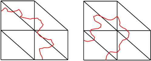
Figure 4: Admissible (left) and non-admissible (right) mesh according to Assumption 4.5. The irregular curve is where the elements are cut by the outer boundary.

Lemma 4.6.

Let $T$ be an element that is cut by the boundary $\partial\Omega$. Under Assumption 4.5 the following Poincaré-Friedrichs type inequality holds

$$\|v\|_{T}\lesssim H\|\nabla v\|_{\omega^{2}_{T}}\quad\text{for all }v\in\mathcal{V}^{f}.$$ (4.18)

Proof.

Let $\widetilde{T}$ be an element which share the vertex $x$ with $T$. Using (4.5) we have that

$$\|v\|_{T}\leq\|v\|_{\omega_{x}^{0}}\lesssim H\|\nabla v\|_{\omega_{x}^{0}}+H^{1/2}\|v\|_{\gamma}\lesssim H\|\nabla v\|_{\omega^{1}_{\widetilde{T}}}\lesssim H\|\nabla v\|_{\omega^{2}_{T}},$$ (4.19)

holds, since $\text{diam}(\omega^{0}_{x})\lesssim H$, $\text{diam}(\omega^{1}_{\widetilde{T}})\lesssim H$ and $\omega_{x}^{0}\subset\omega^{1}_{\widetilde{T}}\subset\omega^{2}_{T}$ choosing $\overline{\gamma}$ as an edge of $\widetilde{T}$ which contains the vertex $x$. ∎

Next we prove local approximation and stability properties for functions which are in some sense close to but outside $\mathcal{V}^{f}$.

Lemma 4.7.

Let $\mathcal{I}_{H}:L^{2}(\Omega_{H})\to\mathcal{V}_{H}$ be the Clément interpolation operator defined by (3.2). If $v=\eta w$, where $\eta$ and $w$ satisfies $0\leq\eta\leq 1$, $\|\nabla\eta\|_{L^{\infty}}\lesssim H^{-1}$, and $w\in\mathcal{V}^{f}$, then the following estimate holds

$$\|H^{-1}(v-\mathcal{I}_{H}v)\|_{T}+\|\nabla\mathcal{I}_{H}v\|_{T}\lesssim\|\nabla w\|_{\omega_{T}^{2}},$$ (4.20)

for all $T\in\mathcal{T}_{H}$.

Proof.

The local approximation and stability properties for an interior element follows directly from Lemma 4.6 together with

$$\|\nabla\eta w\|_{T}\lesssim H^{-1}\|w\|_{T}+\|\nabla w\|_{T}\lesssim\|\nabla w\|_{\omega_{T}^{1}}.$$ (4.21)

Next we investigate the local approximation and stability properties for elements on the boundary. Let $T$ be an element cut by the boundary and $\widetilde{T}$ an interior element sharing vertex $x$ with T. Then the $L^{2}$-stability follows directly from the stability of the interior elements, i.e,

$$\|(P_{x}v)(x)\|_{T} =|(P_{x}v)(x)|\frac{\|1\|_{T}}{\|1\|_{\widetilde{T}}}\|1\|_{\widetilde{T}}\lesssim|(P_{x}v)(x)|\|1\|_{\widetilde{T}}=\|(P_{x}v)(x)\|_{\widetilde{T}}$$ (4.22)

$$\lesssim H^{d/2}\|(P_{x}v)(x)\|_{L^{\infty}(\widetilde{T})}\leq H^{d/2}\|P_{x}v\|_{L^{\infty}(\widetilde{T})}\lesssim\|P_{x}v\|_{\widetilde{T}}$$

$$\leq\|P_{x}v\|_{\omega^{0}_{x}}\leq\|v\|_{\omega^{0}_{x}}\leq\|v\|_{\omega^{1}_{T}}.$$

We obtain

$$\|v-\mathcal{I}_{H}v\|_{T} \lesssim\|v\|_{\omega^{1}_{T}}\lesssim\|w\|_{\omega^{1}_{T}}\lesssim H\|\nabla w\|_{\omega^{2}_{T}},$$ (4.23)

since $w\in\mathcal{V}^{f}$ using Lemma 4.4, $L^{2}$-stability of the interpolation operator, and $w\in\mathcal{V}^{f}$. Similar argument yield

$$\|\nabla\mathcal{I}_{H}v\|_{T} \lesssim\sum_{x\in\mathcal{N}_{T}}H^{-1}\|(P_{x}v)(x)\|_{T}\lesssim\|\nabla w\|_{\omega_{T}^{2}},$$ (4.24)

where $\mathcal{N}_{T}$ is all vertices in element $T$. ∎

4.3 Estimation of the error in the reference finite element solution

We bound the error in the reference finite element solution $u_{h}\in\mathcal{V}^{\Gamma}_{h}$.

Lemma 4.8.

Let $u\in\mathcal{V}$ and $u_{h}\in\mathcal{V}^{\Gamma}_{h}$ be the solutions to (2.2) and (2.9) respectively. Then

$$|||u-u_{h}|||\lesssim\inf_{v_{H}\in\mathcal{V}_{H}}\left(\|H^{-1}(u-v_{H})\|_{\Omega\setminus\omega_{\Gamma}^{k-1}}+|||u-v_{H}|||_{\Omega\setminus\omega_{\Gamma}^{k-1}}\right)+\inf_{v_{h}\in\mathcal{V}_{h}(\omega_{\Gamma}^{k})}|||u-v_{h}|||_{\omega_{\Gamma}^{k}},$$ (4.25)

holds.

Proof.

We split $\Omega$ into the different parts $\Omega\setminus\omega_{\Gamma}^{k}$, $\omega_{\Gamma}^{k}\setminus\omega_{\Gamma}^{k-1}$, and $\omega_{\Gamma}^{k-1}$. Since $\mathcal{V}^{\Gamma}_{h}\subset\mathcal{V}$, we have the best approximation result

$$|||u-u_{h}|||\lesssim|||u-w|||,\qquad\text{for all }w\in\mathcal{V}^{\Gamma}_{h}.$$ (4.26)

Let $\eta\in V_{H}$ be a cut off function, where $\eta|_{\Omega\setminus\omega_{\Gamma}^{k}}=0$, $\eta|_{\omega_{\Gamma}^{k-1}}=1$, and $\|\nabla\eta\|_{L^{\infty}(T)}\lesssim H^{-1}$. We construct $w=v_{H}+\pi_{h}\eta(v_{h}-v_{H})\in\mathcal{V}^{\Gamma}_{h}$ where $v_{H}\in\mathcal{V}_{H}$, $v_{h}\in\mathcal{V}_{h}(\omega_{\Gamma}^{k})$ , and $\pi_{h}$ is the nodal interpolant onto the finite element space $\mathcal{V}_{h}$ and obtain

$$|||u-w|||^{2}=|||u-v_{H}|||^{2}_{\Omega\setminus\omega_{\Gamma}^{k}}+|||u-v_{H}-\pi_{h}\eta(v_{h}-v_{H})|||^{2}_{\omega_{\Gamma}^{k}\setminus\omega_{\Gamma}^{k-1}}+|||u-v_{h}|||^{2}_{\omega_{\Gamma}^{k-1}}.$$ (4.27)

The first and third term are in the right form, see the statement of Lemma 4.8. We turn to the second term. Using the fact that the nodal interpolant $\pi_{h}$ is $H^{1}$-stable for finite polynomial degrees (2 in our case) we obtain

$$|||\pi_{h}\eta(v_{h}-v_{H})|||_{\omega_{\Gamma}^{k}\setminus\omega_{\Gamma}^{k-1}}^{2} \lesssim|||\eta(v_{h}-v_{H})|||_{\omega_{\Gamma}^{k}\setminus\omega_{\Gamma}^{k-1}}^{2}$$ (4.28)

$$=||\nabla(\eta(v_{h}-v_{H}))||^{2}_{\omega_{\Gamma}^{k}\setminus\omega_{\Gamma}^{k-1}}+\kappa||\eta(v_{h}-v_{H})||^{2}_{\partial(\omega_{\Gamma}^{k}\setminus\omega_{\Gamma}^{k-1})\cap\partial\Gamma_{R}}.$$

We have

$$||\nabla(\eta(v_{h}-v_{H}))||_{\omega_{\Gamma}^{k}\setminus\omega_{\Gamma}^{k-1}}$$ (4.29)

$$\qquad\leq||(v_{h}-v_{H})\nabla\eta||_{\omega_{\Gamma}^{k}\setminus\omega_{\Gamma}^{k-1}}+||\eta\nabla(v_{h}-v_{H})||_{\omega_{\Gamma}^{k}\setminus\omega_{\Gamma}^{k-1}}$$

$$\qquad\lesssim H^{-1}||v_{h}-v_{H}||_{\omega_{\Gamma}^{k}\setminus\omega_{\Gamma}^{k-1}}+||\nabla(v_{h}-v_{H})||_{\omega_{\Gamma}^{k}\setminus\omega_{\Gamma}^{k-1}}$$

$$\qquad\lesssim H^{-1}||v_{h}-u+u-v_{H}||_{\omega_{\Gamma}^{k}\setminus\omega_{\Gamma}^{k-1}}+||\nabla(v_{h}-u+u-v_{H})||_{\omega_{\Gamma}^{k}\setminus\omega_{\Gamma}^{k-1}}$$

$$\qquad\lesssim H^{-1}||u-v_{H}||_{\omega_{\Gamma}^{k}\setminus\omega_{\Gamma}^{k-1}}+||\nabla(u-v_{H})||_{\omega_{\Gamma}^{k}\setminus\omega_{\Gamma}^{k-1}}$$

$$\qquad\qquad+H^{-1}||u-v_{h}||_{\omega_{\Gamma}^{k}\setminus\omega_{\Gamma}^{k-1}}+||\nabla(u-v_{h})||_{\omega_{\Gamma}^{k}\setminus\omega_{\Gamma}^{k-1}}.$$

Furthermore

$$\kappa||\eta(v_{h}-v_{H})||^{2}_{\partial(\omega_{\Gamma}^{k}\setminus\omega_{\Gamma}^{k-1})\cap\partial\Omega}\lesssim\kappa||v_{h}-v_{H}||^{2}_{\partial(\omega_{\Gamma}^{k}\setminus\omega_{\Gamma}^{k-1})\cap\partial\Omega}$$ (4.30)

$$\qquad\lesssim\kappa H^{-1}||v_{h}-v_{H}||^{2}_{\omega_{\Gamma}^{k}\setminus\omega_{\Gamma}^{k-1}}+H||\nabla(v_{h}-v_{H})||^{2}_{\omega_{\Gamma}^{k}\setminus\omega_{\Gamma}^{k-1}}.$$

Taking the infimum and using that

$$\inf_{v_{h}\in\mathcal{V}_{h}}\left(H^{-1}||u-v_{h}||_{\omega_{\Gamma}^{k}\setminus\omega_{\Gamma}^{k-1}}+||\nabla(u-v_{h})||_{\omega_{\Gamma}^{k}\setminus\omega_{\Gamma}^{k-1}}\right)$$ (4.31)

$$\qquad\leq\inf_{v_{H}\in\mathcal{V}_{H}}\left(H^{-1}||u-v_{H}||_{\omega_{\Gamma}^{k}\setminus\omega_{\Gamma}^{k-1}}+||\nabla(u-v_{H})||_{\omega_{\Gamma}^{k}\setminus\omega_{\Gamma}^{k-1}}\right),$$

since $h<H$ and $\mathcal{V}_{H}\subset V_{h}$, concludes the proof. ∎

The analysis extends to a non-polygonal boundary if we assume that $h$ is fine enough to approximate the boundary using interpolation onto piecewise affine functions, see e.g. [25].

4.4 Estimation of the error in the global multiscale method

In this section we present and analyze the method with non-localized correctors.

Lemma 4.9.

Let $u_{h}\in\mathcal{V}^{\Gamma}_{h}$ solve (2.9) and $u_{H}\in\mathcal{V}_{H}^{\Gamma}$ solve (3.6), then

$$|||u_{h}-u_{H}|||\lesssim H\|f\|_{\omega_{\Gamma}^{k}}$$ (4.32)

holds.

Proof.

Any $u_{h}\in\mathcal{V}^{\Gamma}_{h}$ can be uniquely written as $u_{h}=u_{H}+u^{\mathrm{f}}$ where $u_{H}\in\mathcal{V}^{\Gamma}_{H}$ and $u^{\mathrm{f}}\in\mathcal{V}^{\mathrm{f}}$. This follows from the result from functional analysis, that if we have a projection $\mathcal{P}:u_{h}\to u_{H}$ onto a closed subspace, there is a unique split $u_{h}=\mathcal{P}u_{h}+(1-\mathcal{P})u_{h}$. For $\mathcal{P}=(1+Q)\mathcal{I}_{H}$, we have $\mathcal{P}\mathcal{V}^{\Gamma}_{h}=\mathcal{V}^{\Gamma}_{H}$ and

$$\mathcal{P}^{2}=(1+Q)\mathcal{I}_{H}(1+Q)\mathcal{I}_{H}=(1+Q)\mathcal{I}_{H}\mathcal{I}_{H}=(1+Q)\mathcal{I}_{H}=\mathcal{P}.$$ (4.33)

We obtain

$$|||u^{\mathrm{f}}|||^{2}=a(u^{\mathrm{f}},u^{\mathrm{f}})=(f,u^{\mathrm{f}})_{L^{2}(\Omega)}=(f,u^{\mathrm{f}}-\mathcal{I}_{H}u^{\mathrm{f}})_{L^{2}(\omega_{\Gamma}^{k})}\lesssim H\|f\|_{\omega_{\Gamma}^{k}}|||u^{\mathrm{f}}|||,$$ (4.34)

which concludes the proof. ∎

4.5 Estimation of the error between global and localized correction

The correctors fulfill the following decay property.

Lemma 4.10 (Decay of correctors).

For any $x\in\mathcal{N}_{I}$ there exist a $0<\gamma<1$ such that the local corrector $Q^{L}_{x}(\varphi_{x})\in\mathcal{V}^{\mathrm{f}}_{L}(\varphi_{x})$ and the global corrector $Q(\varphi_{x})\in\mathcal{V}^{\mathrm{f}}(\varphi_{x})$, which solves (3.9) and (3.5) respectively, fulfills the decay property

$$|||(Q-Q^{L})(v_{H})|||^{2}\leq L^{d}\gamma^{\left\lfloor(L-3)/3\right\rfloor}\sum_{x\in\mathcal{N}_{I}}v_{x}^{2}|||Q\phi_{x}|||^{2},$$ (4.35)

where $\lfloor\cdot\rfloor$ is the floor function which maps a real number to the largest smaller integer.

Proof.

See Appendix A ∎

The localized corrected basis functions fulfill the following stability property.

Lemma 4.11.

Under Assumption 4.5 we have the stability

$$|||\varphi_{x}+Q^{L}(\varphi_{x})|||\lesssim H^{-1}||\varphi_{x}||,$$ (4.36)

for the corrected basis function given any $x\in\mathcal{N}_{I}$.

Proof.

First we will prove that there exist a (non-unique) function $g_{x}\in\mathcal{V}^{f}(\omega^{L}_{x})$ such that $(g_{x}-\varphi_{x})|_{\Gamma_{D}}=0$ and $|||g_{x}|||\lesssim|||\varphi_{x}|||$ for all $x\in\mathcal{N}_{I}$. Given any node $x$ define $w|_{T}=g_{x}-\varphi_{x}$ and $w|_{\Omega\setminus T}=0$ where $T$ is an interior element. The function $w$ have to fulfill the following restriction

$$\mathcal{I}_{H}w=\mathcal{I}_{H}\varphi_{x}=\varphi_{x},$$ (4.37)

which is equivalent to

$$(P_{y}w)(y)=\delta_{xy},$$ (4.38)

where $\delta_{xy}$ is the Kronecker delta function. In order to construct $w$ we perform two a uniform refinements in 2D. A similar construction is possible in 3D using two red-green refinements but we restrict the discussion to 2D for simplicity. Then we have three free nodes in $T$ for a function that is zero on the boundary $\partial T$. We write $w$ as $w=\sum_{j=1}^{d+1}\alpha_{j}\hat{\varphi}_{j}$ where $\varphi_{j}$ are the $P_{1}$ Lagrange basis function associated with the three interior nodes. We can determine $w$ by letting it fulfill

$$\sum_{i,j=1}^{d+1}\alpha_{j}(P_{y_{i}}\hat{\varphi}_{j})(y_{i})=\delta_{x,y_{i}}.$$ (4.39)

The value $(P_{y}\hat{\varphi}_{j})(x)$ can be computed as

$$(P_{y}\hat{\varphi}_{j})(y)=\delta_{y}^{T}(\Pi^{T}M_{H/4}\Pi)^{-1}\Pi^{T}M_{H/4}\hat{\varphi}_{j},$$ (4.40)

where $M_{H/4}$ is a local mass matrix computed on $\omega_{x}^{0}$, $\delta_{x}^{T}=1$ for index $x$ and $0$ otherwise, and $\Pi:\mathcal{V}_{H}\to\mathcal{V}_{H/4}$ is a projection from the finer space onto the coarse. On a quasi-uniform mesh $P_{y}\hat{\varphi}_{j}(y)$ is independent of $H$. Therefore, $\alpha_{j}$ is independent of $H$ and there exist a constant such that

$$||w||\leq C||\varphi_{x}||.$$ (4.41)

This yields

$$|||w|||\lesssim 4H^{-1}||w||\lesssim H^{-1}||\varphi_{x}||.$$ (4.42)

Using the triangle inequality we have

$$|||g_{x}|||\leq|||\varphi_{x}|||+|||w|||\lesssim H^{-1}||\varphi_{x}||.$$ (4.43)

Next we consider the problem: find $Q_{0}\in\mathcal{V}^{f}(\omega^{L}_{x})$ such that

$$a(Q_{0},w)=a(\varphi_{x}-g_{x},w)\quad w\in\mathcal{V}^{f}(\omega^{L}_{x}),$$ (4.44)

where $g_{x}$ satisfies $g_{x}\in\mathcal{V}^{f}(\omega^{L}_{x})$, $(\varphi_{x}-g_{x})|_{\Gamma_{D}}=0$, and $|||g_{x}|||\lesssim|||\varphi_{x}|||$. It is clear that $Q^{L}(\varphi_{x})=Q_{0}+g$. For the stability we obtain

$$|||\varphi_{x}+Q^{L}(\varphi_{x})|||^{2} \leq a(\varphi_{x}+Q^{L}(\varphi_{x}),\varphi_{x}+Q^{L}(\varphi_{x}))=a(\varphi_{x}+Q^{L}(\varphi_{x}),\varphi_{x}+Q_{0}+g)$$ (4.45)

$$=a(\varphi_{x}+Q^{L}(\varphi_{x}),\varphi_{x}+g)\leq|||\varphi_{x}+Q^{L}(\varphi_{x})|||(|||\varphi_{x}|||+|||g_{x}|||)$$

$$\lesssim|||\varphi_{x}+Q^{L}(\varphi_{x})|||\cdot|||\varphi_{x}|||,$$

which concludes the proof. ∎

4.6 Estimation of the error for the localized multiscale method

The a priori results for the localized multiscale method reads.

Theorem 4.12.

Let $u\in\mathcal{V}$ solve (2.2) and $u^{L}_{H}\in\mathcal{V}_{H}^{\Gamma,L}$ solve (3.6). Then under Assumption 4.5 the bound

$$|||u-u^{L}_{H}||| \lesssim\inf_{v\in\mathcal{V}_{H}}\left(\|H^{-1}(u-v)\|_{\Omega\setminus\omega_{\Gamma}^{k-1}}+|||u-v|||_{\Omega\setminus\omega_{\Gamma}^{k-1}}\right)$$ (4.46)

$$\qquad+\inf_{v\in\mathcal{V}_{h}(\omega_{\Gamma}^{k})}|||u-v|||_{\omega_{\Gamma}^{k}}+\|Hf\|_{\omega_{\Gamma}^{k}}+L^{d/2}H^{-1}\gamma^{L}\|f\|,$$

holds for $k\geq 2$.

Proof.

Since $\mathcal{V}_{H}^{\Gamma,L}\subset\mathcal{V}$ we have the best approximation result

$$|||u-u^{L}_{H}|||\leq|||u-v_{H}|||\quad\text{for all }v_{H}\in\mathcal{V}_{H}^{\Gamma,L}.$$ (4.47)

We obtain

$$|||u-u^{L}_{H}|||\leq|||u-u_{h}|||+|||u_{h}-u_{H}|||+|||u_{H}-v_{H}|||,$$ (4.48)

using the triangle inequality. The first and second term is bounded using Lemma 4.8 and 4.9. For the third term we choose $v_{H}=u_{H}+Q(u_{H})$ which gives

$$|||u_{H}-v_{H}|||^{2}=|||Q(u_{H})-Q^{L}(u_{H})|||^{2}\lesssim L^{d}\gamma^{2L}\sum_{x\in\mathcal{N}_{I}}v_{x}^{2}|||Q\phi_{x}|||^{2},$$ (4.49)

using Lemma 4.10. Lemma 4.11 now gives

$$|||u_{H}-v_{H}|||^{2} \lesssim H^{-2}L^{d}\gamma^{2L}\sum_{x\in\mathcal{N}_{I}}u_{H}(x)^{2}\|\varphi_{x}\|^{2}\lesssim L^{d}\gamma^{2L}\|u_{H}\|^{2}$$ (4.50)

$$\lesssim H^{-2}L^{d}\gamma^{2L}|||u_{H}|||^{2}\leq H^{-2}L^{d}\gamma^{2L}||f||^{2},$$

where also a Poincaré-Friedrich inequality has been used. Combining (4.48) and (4.50) concludes the proof. ∎

5 Implementation and conditioning

In this section we will shortly discuss how to implement the proposed method and analyze the conditioning of the matrices. For a more detailed discussion on implementation of LOD see [10].

5.1 Implementation

To compute $Q^{L}(\varphi_{x})$ in (3.9) we impose the extra condition $\mathcal{I}_{H}v=0$ using Lagrangian multipliers. Let $n_{x}$ and $N_{x}$ be the number of fine and coarse degrees of freedom in the patch $\omega^{0}_{x}$. Let $M_{x}$ and $K_{x}$ denote the local mass and stiffness matrix on $\omega^{0}_{x}$ satisfying

$$(v,w)_{\omega^{0}_{x}}\quad\Leftrightarrow\quad\hat{w}^{T}M_{x}\hat{v},$$ (5.1)

and

$$a(v,w)|_{\omega^{0}_{x}}\quad\Leftrightarrow\quad\hat{w}^{T}K_{x}\hat{v},$$ (5.2)

where $v,w\in\mathcal{V}_{h}|_{\omega^{0}_{x}}$ and $\hat{w},\hat{v}\in\mathbb{R}^{n_{x}}$ are the nodal values of $v,w$. We also define the projection matrix $\Pi_{x}:\{v\in\mathcal{V}_{H}(\omega^{0}_{x})\mid\text{supp}(v)\cap\omega^{0}_{x}\neq 0\}\to\mathcal{V}_{h}(\omega^{0}_{x})$ of size $(n_{x}\times N_{x})$ which project a coarse function onto the fine mesh and a Kronecker delta vector of size $N_{x}\times 1$ as $\delta_{x}=(0,\dots,0,1,0,\dots,0)$ where the $1$ is in node $x$. We obtain

$$P_{x}v(x)=0\quad\Leftrightarrow\quad\lambda_{x}^{T}\hat{v}=\delta_{x}^{T}(\Pi_{x}^{T}\widehat{M}_{x}\Pi_{x})^{-1}\Pi^{T}_{x}M_{x}\hat{v}=0.$$ (5.3)

Set $\Lambda=[\lambda_{y_{1}},\lambda_{y_{1}},\dots,\lambda_{y_{N_{x}}}]$, then (3.9) is equivalent to solving the linear system

$$\begin{bmatrix}K_{x}&\Lambda\\ \Lambda^{T}&0\end{bmatrix}\begin{bmatrix}\widehat{Q}^{L}(\varphi_{x})\\ \mu\end{bmatrix}=\begin{bmatrix}-K_{x}\Pi_{x}\widehat{\varphi}_{x}\\ 0\end{bmatrix},$$ (5.4)

where $\widehat{Q}^{L}(\varphi_{x})\in\mathbb{R}^{n_{x}}$ contains the nodal values of $Q^{L}(\varphi_{x})$ and $\mu$ is a Lagrange multiplier. For each coarse node $x$ in $\omega^{0}_{x}$ we need to invert $\Pi_{x}^{T}\widehat{M}_{x}\Pi_{x}$ to assemble (5.4), however since the size is only $(N_{x}\times N_{x})$ it is cheap. The coarse scale stiffness matrix $\widehat{K}$ in (3.10) is given element wise by

$$\widehat{K}_{i,j}=a(\varphi_{j}+Q^{L}(\varphi_{j}),\varphi_{i}+Q^{L}(\varphi_{i})).$$ (5.5)

We save the nodal values of the corrected basis

$$\Phi=\begin{bmatrix}\varphi_{y_{1}}+\widehat{Q}^{L}(\varphi_{y_{1}}),\varphi_{y_{2}}+\widehat{Q}^{L}(\varphi_{y_{2}})\dots,\varphi_{y_{N}}+\widehat{Q}^{L}(\varphi_{y_{N}})\end{bmatrix}.$$ (5.6)

Given the fine scale stiffness matrix $K$ and the collection of corrected basis functions $\Phi$, we can compute the coarse stiffness matrix as

$$\widehat{K}=\Phi^{T}K\Phi,$$ (5.7)

and the linear system (3.10) is computed as

$$\widehat{K}\hat{u}^{\Gamma,L}_{H}=b,$$ (5.8)

where $\hat{u}^{\Gamma,L}_{H}$ is the nodal values of $\hat{u}^{\Gamma,L}_{H}$ and $b$ correspond to the right hand side $b_{y_{1}}=(f,\varphi_{y_{1}}+\widehat{Q}^{L}(\varphi_{y_{1}}))$. However, the fine stiffness matrix does not have to be assembled globally. If a Petrov-Galerkin formulation is used, further savings can be made [9].

5.2 Conditioning

The Euclidean matrix norm is defined as

$$||A||_{N}=\sup_{0\neq v\in\mathbb{R}^{N}}\frac{|Av|_{N}}{|v|_{N}},$$ (5.9)

where $\langle v,w\rangle=\sum_{i=1}^{N}v(x_{i})w(x_{i})$ and $|v|_{N}=\sqrt{\langle v,v\rangle}$.

Theorem 5.1.

The bound

$$\kappa=\|\widehat{K}\|_{N}\|\widehat{K}^{-1}\|_{N}\lesssim H^{-2},$$ (5.10)

on the condition number $\kappa$ holds.

Proof.

To prove the bound of the condition number we use the following three properties.

1. An inverse type inequality for the modified basis functions. We have

   $$|||\varphi_{i}+Q(\varphi_{i})|||\lesssim H^{-1}\|\varphi_{i}\|,$$ (5.11)

   from Lemma 4.11.

2. A Poincaré-Friedrich type inequality on the full domain, see Section 4.1.

3. An equivalence between the Euclidean norm and the $L^{2}$-norm. We have that

   $$\|v\|^{2} \leq\sum v_{i}^{2}\|\varphi_{i}+Q(\varphi_{i})\|^{2}\lesssim\sum v_{i}^{2}(\|\varphi_{i}\|+\|Q(\varphi_{i})-\mathcal{I}_{H}Q(\varphi_{i})\|)^{2}$$ (5.12)

   $$\lesssim\sum v_{i}^{2}(\|\varphi_{i}\|+H\|\nabla Q(\varphi_{i})\|)^{2}$$

   $$\lesssim\sum v_{i}^{2}(\|\varphi_{i}\|+H\|\nabla\varphi_{i}\|+H\|\nabla(\varphi_{i}-Q(\varphi_{i}))\|)^{2}$$

   $$\lesssim\sum v_{i}^{2}\|\varphi_{i}\|^{2}\lesssim H^{d}|v|_{N},$$

   and

   $$|v|_{N}^{2}=\sum_{i=1}^{N}v_{i}^{2}\lesssim H^{-d}\sum_{i=1}^{N}v_{i}^{2}\|\varphi_{i}\|^{2}\lesssim H^{-d}\|\sum_{i=1}^{N}v_{i}\varphi_{i}\|^{2}=H^{-d}\|\mathcal{I}_{H}v\|^{2}\lesssim H^{-d}\|v\|^{2}.$$ (5.13)

   holds, hence $|v|_{N}\sim H^{-d/2}\|v\|$.

We have

$$|\widehat{K}v|_{N}=\sup_{0\neq w\in\mathbb{R}^{N}}\frac{|\langle\widehat{K}v,w\rangle|}{|w|_{N}}=\sup_{0\neq w\in\mathbb{R}^{N}}\frac{|a(v,w)|}{|w|_{N}}=\sup_{0\neq w\in\mathbb{R}^{N}}\frac{|||v|||\cdot|||w|||}{|w|_{N}}\leq H^{d-2}|v|_{N},$$ (5.14)

using property 1) and 3). Also

$$|\widehat{K}^{-1}v|_{N}^{2} =H^{-d}\|\widehat{K}^{-1}v\|^{2}\leq C_{\mathrm{PF}}H^{-d}|||\widehat{K}^{-1}v|||^{2}$$ (5.15)

$$\leq H^{-d}\langle\widehat{K}\widehat{K}^{-1}v,\widehat{K}^{-1}v\rangle\leq H^{-d}|v|_{N}\cdot|\widehat{K}^{-1}v|_{N},$$

using property 2) and 3). The proof is concluded by taking the supremum over $v$. ∎

6 Numerical experiments

In the following section we present some numerical experiments that verifies our analytical results. In all the experiments we fix the right hand side to $f=1$ and the localization parameter $L=\lceil 1.5\log_{2}(H^{-1})\rceil$.

6.1 Accuracy on fractal shaped domain

We consider the domain in Figure 2. We use homogeneous Dirichlet boundary conditions on the most left, down, and right hand side boundaries and Robin boundary condition with $\kappa=10$ on the rest, see Figure 5.

Figure 5: The fractal computational domain used in Section 6.1. We use homogeneous Dirichlet boundary conditions on the boundary segments marked by a thicker line and Robin boundary conditions elsewhere.

We compute localized correctors in the full domain. The reference solution is computed using $h=2^{-9}$. As seen in Figure 6, a even higher convergence rate than linear convergence to the reference solution is observed. We also see that the correct scaling of the condition number with respect to the coarse mesh parameter $H$.

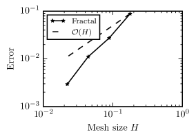
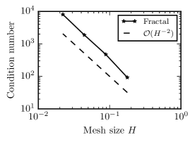
Figure 6: The convergence rate to the reference solution in relative energy norm (left) and the scaling of the condition number (right) for the fractal domain in Figure 6.

6.2 Locally added correctors around singularities

Let us consider two different domains, a domain with a re-entrant corner $([0,1]\times[0,1])\backslash([0.5,1]\times[0,0.5])$ and a slit-domain $([0,1]\times[0,1])\backslash([0.5,0.5]\times[0,0.5])$ with homogeneous Dirichlet boundary condition. We only compute correctors in a vicinity of the singularities, and denote this domain $\omega^{k}$. The size of $\omega^{k}$ can be determined by the size of $|u|_{H^{2}(\omega^{k})}$ (see Section 2.2), i.e., how fast the singularity decay away from the boundary. We choose $\omega^{k}$ as in Figure 7.

As seen in Figure 8, the correct convergence rates to the reference solutions and the correct scaling of the condition number are observed for both singularities.

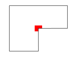
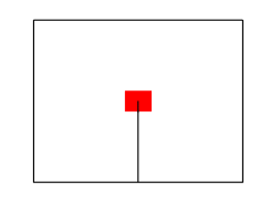
Figure 7: The marked area $\omega^{k}$ is where the finite element space is enriched, for domain with a re-entrant corner (left) and domain with a slit (right).

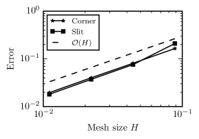
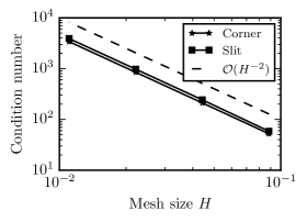
Figure 8: The convergence rate to the reference solution in relative energy norm (left) and scaling of the condition number (right) for the re-entrant corner and the slit domain.

6.3 Locally add correctors around saw tooth boundary

Let us consider a unit square where one of the boundaries are cut as a saw tooth and where correctors are only computed in a vicinity of the saw teeth shown in Figure 9. On all the non saw tooth boundaries we use homogeneous Dirichlet boundary conditions. On the saw tooth boundary we test both homogeneous Dirichlet and Neumann boundary condition. We observe the correct convergence (although the Neumann case is a bit more sensitive and might need slightly larger domain where correctors are computed) and scaling of the condition number, see Figure 10.

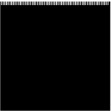
Figure 9: We consider the saw tooth domain (left). The marked area (right) is where the finite element space is enriched.

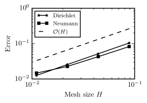
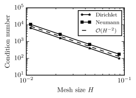
Figure 10: The convergence rate to the reference solution in relative energy norm (left) and the scaling of the condition number (right) for the saw tooth shaped boundary using different boundary condition on the saw tooths.

6.4 Accuracy and conditioning on cut domains

Let us consider a domain with a re-entrant corner $\Omega=([0,1]\times[0,1])\backslash([0.5,1]\times[0,0.5])$. We want to investigate how the location of the boundary relative to the coarse background mesh affects the accuracy in the approximation and the conditioning of the matrix. We fix the coarse $H=2^{-3}$ and fine $h=2^{-8}$ mesh sizes and consider three different setups of boundary condition, homogeneous Dirichlet on the whole boundary, homogeneous Dirichlet on the cut elements and homogeneous Neumann otherwise, and homogeneous Neumann on the cut elements and homogeneous Dirichlet otherwise. We will cut the coarse mesh in two different ways, 1) with a horizontal cut and 2) a circular cut around the reentered corner, see Figure 11. The errors are measured in energy norm. The results are presented in Table 1 and 2. We conclude that neither the error nor the conditioning are sensitive to how the domain is cut.

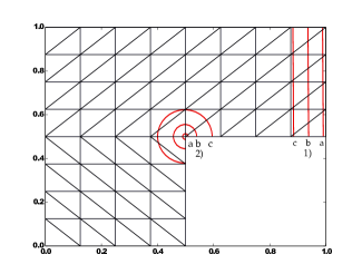
Figure 11: A given background mesh that is cut in two different ways 1) and 2) with different size of the cut a), b), and c).

$\Gamma_{cut}$	$\partial\Omega\setminus\Gamma_{cut}$	$e_{\mathrm{rel}}(a)$	$e_{\mathrm{rel}}(b)$	$e_{\mathrm{rel}}(c)$
D	D	$0.059$	$0.057$	$0.056$
D	N	$0.018$	$0.019$	$0.020$
N	D	$0.063$	$0.055$	$0.053$
		$\mathrm{cond}(a)$	$\mathrm{cond}(b)$	$\mathrm{cond}(c)$
D	D	$9.85$	$10.10$	$13.63$
D	N	$299.75$	$282.26$	$353.27$
N	D	$10.537$	$10.79$	$11.47$

Table 1: For cut $1$ we have $L\cap[0,1-r]\times[0,1]$, where $r=\{h,0.5H,H-h\}$ in $a)$, $b)$, and $c)$, respectively. The errors measured in relative energy norm and condition number of the coarse stiffness matrix are presented. We try the different boundary conditions, $D$ (Dirichlet) and $N$ (Neumann), on the boundary segement $\Gamma_{cut}$, which cuts the elements.

$\Gamma_{cut}$	$\partial\Omega\setminus\Gamma_{cut}$	$e_{\mathrm{rel}}(a)$	$e_{\mathrm{rel}}(b)$	$e_{\mathrm{rel}}(c)$
D	D	$0.060$	$0.064$	$0.073$
D	N	$0.0205$	$0.035$	$0.048$
N	D	$0.060$	$0.057$	$0.059$
		$\mathrm{cond}(a)$	$\mathrm{cond}(b)$	$\mathrm{cond}(c)$
D	D	$9.80$	$9.23$	$7.03$
D	N	$246.99$	$107.52$	$59.67$
N	D	$9.90$	$11.44$	$12.16$

Table 2: For cut $2$ we have $L\setminus B(x_{0},r)$ for a ball $B$ centered in $x_{0}=(0.5,0.5)$ and with radius $r$, where $r=\{h,0.5H,H\}$ in $a)$, $b)$, and $c)$, respectively. The errors measured in energy norm and condition number of the coarse stiffness matrix are presented. We try the different boundary conditions, $D$ (Dirichlet) and $N$ (Neumann), on the boundary segement $\Gamma_{cut}$, which cuts the elements.

Appendix A Proofs

In the appendix we present the proof of Lemma 4.10.

Proof of Lemma 4.10.

We will make frequent use of the cut off function $\eta_{x}^{k-1,k}$ which satisfy $\eta_{x}^{k-1,k}=0$ in $\omega_{x}^{k-1}$, $\eta_{x}^{k-1,k}=1$ in $\Omega\setminus\omega_{x}^{k}$, and $\|\nabla\eta_{x}^{k-1,k}\|_{L^{\infty}(\Omega)}\lesssim H^{-1}$. Given $v_{H}\in\mathcal{V}_{H}$ with nodal values $v_{x}$ we define define $e=(Q-Q^{L})(v_{H})$ and $e=\sum_{x\in\mathcal{N}_{I}}e_{x}$ where $e_{x}=(Q-Q^{L}_{x})v_{x}\varphi_{x}$, we obtain

$$|||e|||^{2} \lesssim a(e,e)=\sum_{x\in\mathcal{N}_{I}}a\left((Q_{x}-Q^{L}_{x})v_{x}\varphi_{x},e\right)=\sum_{x\in\mathcal{N}_{I}}a\left(e_{x},e-\tilde{v}_{x}\right)$$ (A.1)

for $\tilde{v}_{x}$ which satisfy

$$a(e_{x},\tilde{v}_{x})=0.$$ (A.2)

We choose $\tilde{v}_{x}=\eta_{x}^{L+2,L+1}e-\mathcal{I}_{H}\eta_{x}^{L+2,L+1}e+g_{x}$ where $\mathcal{I}_{H}g_{x}=0$, $g_{x}|_{\partial\Omega}=\mathcal{I}_{H}\eta_{x}^{L+2,L+1}e$, and $|||g_{x}|||\leq|||\mathcal{I}_{H}\eta_{x}^{L+2,L+1}e|||$. It is possible to construct $g_{x}$ with the given properties, see the proof of Lemma 4.11. Equation (A.2) now follows since $\tilde{v}_{x}\in\mathcal{V}^{\mathrm{f}}$ and $\text{supp}(\tilde{v}_{x})\cap\text{supp}(Q^{L}_{x}(v))=0$. For each $x\in\mathcal{N}_{I}$, we obtain

$$a\left(e_{x},e-\tilde{v}_{x}\right)\leq|||e_{x}|||\cdot|||e-\tilde{v}_{x}|||$$ (A.3)

where we split

$$|||e-\tilde{v}_{x}|||\leq|||e-\eta_{x}^{L+2,L+1}e|||+|||\eta_{x}^{L+2,L+1}e-\tilde{v}_{x}|||.$$ (A.4)

The first term in (A.4) can be bounded as

$$|||(1-\eta_{T}^{L+2,L+1})e|||^{2}_{\omega_{x}^{L+2}}\lesssim\|\nabla(1-\eta_{T}^{L+2,L+1})e\|^{2}_{\omega_{x}^{L+2}}+\|\kappa(1-\eta_{T}^{L+2,L+1})e\|^{2}_{\partial\omega_{x}^{L+2}\cap\Gamma}$$ (A.5)

$$\qquad\leq\|\nabla e\|^{2}_{\omega_{x}^{L+2}}+H^{-1}\|e\|^{2}_{\omega_{x}^{L+2}}+\|\kappa(1-\eta_{T}^{L+2,L+1})e\|^{2}_{\partial\omega_{x}^{L+2}\cap\Gamma}$$

$$\qquad\leq|||e|||^{2}_{\omega_{x}^{L+3}}$$

using the product rule, inverse estimates, and interpolation estimates. The second term in (A.4) can be bounded as

$$|||\eta_{x}^{L+2,L+1}e-\tilde{v}_{x}|||^{2}=\|\nabla\mathcal{I}_{H}(\eta^{L}_{T}e)\|^{2}+\|\kappa\mathcal{I}_{H}(\eta^{L}_{T}e)\|^{2}_{\Gamma}\lesssim|||e|||^{2}_{\omega^{L+4}_{x}}$$ (A.6)

where we used

$$\|\nabla\mathcal{I}_{H}(\eta_{x}^{L+2,L+1}e)\|^{2} =\|\nabla(\mathcal{I}_{H}\eta_{x}^{L+2,L+1}e)\|^{2}_{\omega^{L+3}_{x}\setminus\omega^{L}_{x}}\lesssim H^{-2}\|e\|^{2}_{\omega^{L+3}_{x}\setminus\omega^{L}_{x}}$$ (A.7)

$$\leq|||e|||^{2}_{\omega^{L+4}_{x}\setminus\omega^{L-1}_{x}}\leq|||e|||^{2}_{\omega^{L+4}_{x}}$$

and

$$\|\kappa\mathcal{I}_{H}(\eta_{x}^{L+2,L+1}e)\|^{2}_{\Gamma_{x}^{L}} =\sum_{E\in\Gamma_{x}^{L}}\|\kappa\mathcal{I}_{H}(\eta_{x}^{L-2,L-1}e)\|^{2}_{E}\leq\kappa H^{-1}\|\mathcal{I}_{H}(\eta_{\omega^{L-1}_{x}}e)\|^{2}_{\omega_{x}^{L+3}}$$ (A.8)

$$\leq\kappa H^{-1}\|e-\mathcal{I}_{H}e\|^{2}_{\omega_{x}^{L+3}}\leq\kappa H\|\nabla e\|^{2}_{\omega_{x}^{L+4}}\leq|||e|||^{2}_{\omega^{L+4}_{x}}$$

which follows from Lemma 4.7 and that $\kappa\lesssim H^{-1}$. Hence, combining (A.1), (A.4), (A.5), and (A.6) we obtain

$$|||e|||^{2} \lesssim\sum_{x\in\mathcal{N}_{I}}|||e_{x}|||\cdot|||e|||_{\omega^{L+4}_{x}}\lesssim L^{d}\left(\sum_{x\in\mathcal{N}_{I}}|||e_{x}|||^{2}\right)^{1/2}|||e|||$$ (A.9)

that is

$$|||e|||^{2}\lesssim L^{d}\sum_{x\in\mathcal{N}_{I}}|||e_{x}|||^{2}$$ (A.10)

We use $\tilde{w}_{x}=(1-\eta_{x}^{L-1,L-2})Q(v_{x}\varphi_{x})+\mathcal{I}_{H}\eta_{x}^{L-1,L-2}Q(v_{x}\varphi_{x})+\tilde{g}_{x}\in\mathcal{V}^{f}(\omega^{L}_{x})$ where we use the same construction of $\tilde{g}_{x}$ as for $g_{x}$ and obtain

$$|||e_{x}|||^{2}\leq a(e_{x},e_{x}) =a(e_{x},Q(v_{x}\varphi_{x})-\tilde{w}_{x})$$ (A.11)

$$=a(e_{x},\eta_{x}^{L-1,L-2}Q(v_{x}\varphi_{x})-\mathcal{I}_{H}\eta_{x}^{L-1,L-2}Q(v_{x}\varphi_{x})+g_{x})$$

$$\lesssim|||e_{x}|||(|||\eta_{x}^{L-1,L-2}Q(v_{x}\varphi_{x})|||+|||\mathcal{I}_{H}\eta_{x}^{L-1,L-2}Q(v_{x}\varphi_{x})|||)$$

$$\lesssim|||e_{x}|||\cdot|||Q(v_{x}\varphi_{x})|||_{\Omega\setminus\omega_{x}^{L-3}}$$

and hence

$$|||e_{x}|||\leq|v_{x}||||Q(\varphi_{x})|||_{\Omega\setminus\omega_{x}^{L-3}}$$ (A.12)

Next we construct a recursive scheme which will be used to show the decay. We obtain

$$|||Q\varphi_{x}|||_{\Omega\setminus\omega^{k}_{x}}^{2} \leq\int_{\Omega}\eta_{T}^{k,k-1}\nabla Q\varphi_{x}\nabla Q\varphi_{x}\,\mathrm{d}x+\int_{\Gamma_{R}}\eta_{T}^{k,k-1}\kappa Q\phi_{x}Q\varphi_{x}\,\mathrm{d}S$$ (A.13)

$$=\int_{\Omega}\nabla Q\varphi_{x}\nabla(\eta_{T}^{k,k-1}Q\varphi_{x})\,\mathrm{d}x+\int_{\Gamma_{R}}\kappa Q\varphi_{x}(\eta_{T}^{k,k-1}Q\varphi_{x})\,\mathrm{d}S$$

$$\qquad-\int_{\Omega}Q\varphi_{x}\nabla Q\varphi_{x}\nabla\eta_{T}^{k,k-1}\,\mathrm{d}x$$

$$=a(Q\varphi_{x},\eta_{T}^{k,k-1}Q\varphi_{x})-\int_{\Omega}Q\varphi_{x}\nabla Q\varphi_{x}\nabla\eta_{T}^{k,k-1}\,\mathrm{d}x.$$

The first term in (A.13) can be bounded as

$$a(Q\varphi_{x},\eta_{x}^{k,k-1}Q\varphi_{x}) =a(Q\varphi_{x},\eta_{x}^{k,k-1}Q\varphi_{x}-\mathcal{I}_{H}\eta_{x}^{k,k-1}Q\varphi_{x}-\hat{g}_{x})+a(Q\varphi_{x},\mathcal{I}_{H}\eta_{x}^{k,k-1}Q\varphi_{x}+\hat{g}_{x})$$ (A.14)

$$=a(Q\varphi_{x},\mathcal{I}_{H}\eta_{x}^{k,k-1}Q\varphi_{x}+\hat{g}_{x})\lesssim|||Q\varphi_{x}|||_{\omega^{k}_{x}\setminus\omega^{k-1}_{x}}|||\mathcal{I}_{H}\eta_{x}^{k,k-1}Q\varphi_{x}|||$$

$$\lesssim|||Q\varphi_{x}|||_{\omega^{k}_{x}\setminus\omega^{k-1}_{x}}|||Q\varphi_{x}||||_{\omega^{k+1}_{x}\setminus\omega^{k-2}_{x}}|||Q\varphi_{x}|||_{\omega^{k+1}_{x}\setminus\omega^{k-2}_{x}}^{2}$$

where again we construct $\hat{g}_{x}$ such that $|||\hat{g}_{x}|||\lesssim|||\mathcal{I}_{H}\eta_{x}^{k,k-1}Q\varphi_{x}|||$ and use Lemma 4.7. The second term is bounded as

$$\int_{\Omega}Q\varphi_{x}\nabla Q\varphi_{x}\nabla\eta_{x}^{k,k-1}\,\mathrm{d}x \leq H^{-1}\|Q\varphi_{x}-\mathcal{I}_{H}Q_{x}v\|_{\omega^{k}_{x}\setminus\omega^{k-1}_{x}}|||Q\varphi_{x}|||_{\omega^{k}_{x}\setminus\omega^{k-1}_{x}}$$ (A.15)

$$\lesssim|||Q\varphi_{x}|||_{\omega^{k+1}_{x}\setminus\omega^{k-2}_{x}}|||Q\varphi_{x}||||_{\omega^{k+1}_{x}\setminus\omega^{k-2}_{x}}\leq|||Q\varphi_{x}|||_{\omega^{k+1}_{x}\setminus\omega^{k-2}_{x}}^{2}$$

Combining (A.13), (A.14), and (A.15) we obtain

$$|||Q\varphi_{x}|||_{\Omega\setminus\omega^{k}_{x}}^{2} \leq C_{1}|||Q\varphi_{x}|||_{\omega^{k+1}_{x}\setminus\omega^{k-2}_{x}}^{2}=C_{1}\left(|||Q\varphi_{x}|||_{\Omega\setminus\omega^{k-2}_{x}}^{2}-|||Q\varphi_{x}|||_{\Omega_{x}\setminus\omega^{k+1}_{x}}^{2}\right)$$ (A.16)

$$\leq C_{1}\left(|||Q\varphi_{x}|||_{\Omega\setminus\omega^{k-2}_{x}}^{2}-|||Q\varphi_{x}|||_{\Omega_{x}\setminus\omega^{k}_{x}}^{2}\right)$$

and hence

$$|||Q(v_{x}\varphi_{x})|||_{\Omega\setminus\omega^{k}_{x}}^{2}\leq\gamma|||Q(v_{x}\varphi_{x})|||_{\Omega\setminus\omega^{k-2}_{x}}^{2},$$ (A.17)

where $\gamma=\frac{C_{1}}{1+C_{1}}$. Using (A.17) recursively we obtain

$$|||Q\varphi_{x}|||_{\Omega\setminus\omega^{L-3}}^{2}\leq\gamma^{k}|||Q\varphi_{x}|||_{\Omega\setminus\omega^{L-3(k+1)}_{x}}^{2}$$ (A.18)

$$\Leftrightarrow |||Q\varphi_{x}|||_{\Omega\setminus\omega^{L-3}}^{2}\leq\gamma^{\left\lfloor(L-3)/3\right\rfloor}|||Q\varphi_{x}|||_{\Omega\setminus\omega^{0}_{x}}^{2}\leq\gamma^{\left\lfloor(L-3)/3\right\rfloor}|||Q\varphi_{x}|||^{2}.$$

Combing (A.9), (A.12), and, (A.18) we get

$$|||e|||^{2}\lesssim L^{d}\gamma^{\left\lfloor(L-3)/3\right\rfloor}\sum_{x\in\mathcal{N}_{I}}v_{x}^{2}|||Q\varphi_{x}|||^{2}$$ (A.19)

which concludes the lemma. ∎

References

- [1] R. A. Adams. Sobolev spaces. Academic Press, 1975. Pure and Applied Mathematics, Vol. 65.
- [2] I. Babuška, G. Caloz, and J. E. Osborn. Special finite element methods for a class of second order elliptic problems with rough coefficients. SIAM J. Numer. Anal., 31(4):945–981, 1994.
- [3] I. Babuška and J. E. Osborn. Can a finite element method perform arbitrarily badly? Math. Comp., 69(230):443–462, 2000.
- [4] D. Brown and D. Peterseim. A Multiscale Method for Porous Microstructures. Multiscale Model. Simul., 14(3):1123–1152, 2016.
- [5] E. Burman, S. Claus, P. Hansbo, M. G. Larson, and A. Massing. Cutfem: Discretizing geometry and partial differential equations. International Journal for Numerical Methods in Engineering, 2014.
- [6] W. E and B. Engquist. The heterogeneous multiscale methods. Commun. Math. Sci., 1(1):87–132, 2003.
- [7] D. Elfverson, E. H. Georgoulis, and A. Målqvist. An adaptive discontinuous Galerkin multiscale method for elliptic problems. Multiscale Model. Simul., 11(3):747–765, 2013.
- [8] D. Elfverson, E. H. Georgoulis, A. Målqvist, and D. Peterseim. Convergence of a discontinuous Galerkin multiscale method. SIAM J. Numer. Anal., 51(6):3351–3372, 2013.
- [9] D. Elfverson, V. Ginting, and P. Henning. On multiscale methods in petrov–galerkin formulation. Numerische Mathematik, pages 1–40, 2015.
- [10] C. Engwer, P. Henning, A. Målqvist, and D. Peterseim. Efficient implementation of the localized orthogonal decomposition method. ArXiv e-prints, 2016.
- [11] T.-P. Fries and T. Belytschko. The extended/generalized finite element method: an overview of the method and its applications. Internat. J. Numer. Methods Engrg., 84(3):253–304, 2010.
- [12] R. Glowinski, T.-W. Pan, and J. Periaux. A fictitious domain method for dirichlet problem and applications. Computer Methods in Applied Mechanics and Engineering, 111(3):283 – 303, 1994.
- [13] W. Hackbusch and S. A. Sauter. Composite finite elements for the approximation of PDEs on domains with complicated micro-structures. Numer. Math., 75(4):447–472, 1997.
- [14] T. Y. Hou and X.-H. Wu. A multiscale finite element method for elliptic problems in composite materials and porous media. J. Comput. Phys., 134(1):169–189, 1997.
- [15] T. J. R. Hughes, G. R. Feijóo, L. Mazzei, and J.-B. Quincy. The variational multiscale method—a paradigm for computational mechanics. Comput. Methods Appl. Mech. Engrg., 166(1-2):3–24, 1998.
- [16] M. G. Larson and A. Målqvist. Adaptive variational multiscale methods based on a posteriori error estimation: energy norm estimates for elliptic problems. Comput. Methods Appl. Mech. Engrg., 196(21-24):2313–2324, 2007.
- [17] A. L. Madureira. A multiscale finite element method for partial differential equations posed in domains with rough boundaries. Math. Comp., 78(265):25–34, 2009.
- [18] A. L. Madureira and F. Valentin. Asymptotics of the Poisson problem in domains with curved rough boundaries. SIAM J. Math. Anal., 38(5):1450–1473 (electronic), 2006/07.
- [19] A. Målqvist. Multiscale methods for elliptic problems. Multiscale Model. Simul., 9(3):1064–1086, 2011.
- [20] A. Målqvist and D. Peterseim. Localization of elliptic multiscale problems. Math. Comp., 83(290):2583–2603, 2014.
- [21] A. Målqvist and D. Peterseim. Computation of eigenvalues by numerical upscaling. Numerische Mathematik, 130(2):337–361, 2015.
- [22] H. Owhadi, L. Zhang, and L. Berlyand. Polyharmonic homogenization, rough polyharmonic splines and sparse super-localization. ESAIM Math. Model. Numer. Anal., 48(2):517–552, 2014.
- [23] C. Pechstein and R. Scheichl. Weighted Poincaré inequalities. IMA J. Numer. Anal., 33(2):652–686, 2013.
- [24] D. Peterseim. Eliminating the pollution effect in Helmholtz problems by local subscale correction. Math. Comp., 2016. Also available as INS Preprint No. 1411.
- [25] R. Scott. Interpolated boundary conditions in the finite element method. SIAM J. Numer. Anal., 12:404–427, 1975.
- [26] R. Verführt. A review of a posteriori error estimation and adaptive mesh-refinement techniques. Advances in numerical mathematics. Wiley, 1996.
- [27] H. Yserentant. Coarse grid spaces for domains with a complicated boundary. Numer. Algorithms, 21(1-4):387–392, 1999.