Automatic Loop Kernel Analysis and
Performance Modeling With Kerncraft

Abstract

Analytic performance models are essential for understanding the performance characteristics of loop kernels, which consume a major part of CPU cycles in computational science. Starting from a validated performance model one can infer the relevant hardware bottlenecks and promising optimization opportunities. Unfortunately, analytic performance modeling is often tedious even for experienced developers since it requires in-depth knowledge about the hardware and how it interacts with the software. We present the “Kerncraft” tool, which eases the construction of analytic performance models for streaming kernels and stencil loop nests. Starting from the loop source code, the problem size, and a description of the underlying hardware, Kerncraft can ideally predict the single-core performance and scaling behavior of loops on multicore processors using the Roofline or the Execution-Cache-Memory (ECM) model. We describe the operating principles of Kerncraft with its capabilities and limitations, and we show how it may be used to quickly gain insights by accelerated analytic modeling.

1 Introduction

This paper is concerned with analytic performance modeling on the CPU core and chip level. We define an analytic performance model as a simplified mathematical description of the interaction between program code (“software”) and hardware, constructed with the goal in mind to understand the dominating bottlenecks in program execution performance. The fundamental resources required for the execution of any program are instructions and data; thus, in order to predict the time it takes to execute a program one must have models for how instructions are executed in the CPU core(s) and how data travels through the memory hierarchy. It should be emphasized that the more accurate a model the more specific to a CPU architecture it will be. However, even simple analytic models can lead to surprising and useful insights.

A simple, very optimistic model for instruction execution would assume perfect out-of-order processing, perfect pipelining, and no dependencies, with all required data residing in the L1 cache. Instructions would be distributed among the suitable pipelines, and the pipeline that takes the longest time to execute its instructions would determine the runtime of the code. We term this model the throughput model (TP). If dependencies along the critical path are taken into account one arrives at a more pessimistic model, the critical path model (CP). In reality, and especially for loop-based codes where some “steady state” execution may be assumed, the actual runtime will be in between the TP and CP models as long as no other bottlenecks apply, such as instruction cache misses, instruction throughput limitations, or data transfers beyond the L1 cache.

The Roofline model (see Sect. 2.2) and the Execution-Cache-Memory (ECM) model (see Sect. 2.3) are two useful performance models for steady-state loop codes that build on an instruction execution model but also take data transfers into account. Both models may require considerable effort and experience to construct in complicated cases (e.g., when the code is composed of many loops, or when a loop has a complicated structure). In this work we demonstrate a software tool, Kerncraft, that can automatically construct these models from a C code formulation and a suitable hardware description without actually executing the code. We restrict ourselves to streaming and stencil loop nests, where the data access patterns can be statically determined at compile time. It is not our intention to assess the usefulness or accuracy of the models themselves, although some examples will be given that highlight their capabilities.

Supporting tools are employed to determine parameters that are required as model input in the machine description. We use the LIKWID tool suite [19] for most of these tasks: The machine topology, i.e., information about core and cache sharing, ccNUMA structure, cache sizes, etc., is extracted from the output of likwid-topology. Achievable bandwidths to caches and main memory are measured with the likwid-bench tool [20], since it provides a controlled and compiler-independent environment for building tailored benchmark loops.

Any analytic performance model must be checked for validity by comparing its predictions with measurements on the target hardware. The validation of predictions with measurements is an integral part of the Kerncraft tool.

This paper is organized as follows: In Sect. 2 we briefly describe the components of the performance models (in-core model, Roofline, and ECM) supported by Kerncraft. Section 3 introduces the hardware and software used for all experiments. Details about the structure of the Kerncraft tool and its concrete implementation are given in Sect. 4. In Sect. 5 we evaluate the tool using streaming and stencil loop codes, and Sect. 7 gives a summary and an outlook to future work.

The current version of Kerncraft is available for download at https://github.com/RRZE-HPC/kerncraft.

2 Background

In this section we briefly describe the required components for steady-state loop performance modeling: the in-core execution model, the Roofline model, the ECM model, and approaches for model validation.

2.1 In-core execution modeling

In simple cases the throughput and critical path modeling described above can be done by hand. Listing 1 shows the source code for a scalar product in double precision.

Listing 1: Scalar product in double precision

⬇

double a[], b[], s=0.;

for(i=0; i<N; ++i)

s += a[i] * b[i];

On a CPU with a three-stage ADD pipeline, the (scalar) naive code, i.e., without any unrolling and modulo variable expansion, would be limited by the dependency on the summation variable s. Hence, the core would execute one floating-point operation (flop) every $3\,\mbox{cy}$, which is also the CP prediction for one loop iteration. The TP prediction would be $2\,\mbox{cy}$ if the core can execute one LOAD, one ADD, and one MULT instruction per cycle. With appropriate unrolling and modulo variable expansion this limit can be achieved in practice if no other bottlenecks apply.

With more complicated code the pencil-and-paper analysis becomes tedious and error-prone. One solution, albeit limited to Intel architectures, is the Intel Architecture Code analyzer (IACA) [12], which provides TP and CP predictions for assembly code sections. In Kerncraft we use the IACA TP output (and optionally the CP output) as the in-core component in the ECM and Roofline models. IACA also provides information about port utilization and points out a front-end bottleneck in case the code would need more concurrency than what is supported by the instruction decoders.

2.2 Roofline model

The Roofline model is optimistic by design, i.e., it yields an absolute lower execution time limit for a loop. The ideas behind the model have been in use since the 1980s [16, 3, 9], but it was popularized (and got its current name) by Williams et al. in 2009 [23]. It is based on the assumption that performance is limited either by data transfers from a certain memory hierarchy level or by the computational (arithmetic) work, whichever takes longer. This implies that all data transfers perfectly overlap with computation. In order to apply the model, the data volume from and to each memory hierarchy level $k$, $\beta_{k}$, needs to be assessed and put in relation to the achievable peak bandwidth $B_{k}$ of that level. Their ratio $T_{k}=\beta_{k}/B_{k}$ determines the data transfer time for level $k$. To have a formulation that is, as far as possible, independent of the clock frequency setting, bandwidths are best given in bytes per clock cycle.

In a naive approach the time required for computation can be calculated by dividing the work $\phi$ (usually flops, but any other well-defined metric will do) by the applicable computational peak performance $P_{\mathrm{peak}}$ of the code at hand: $T_{\mathrm{core}}=\phi/P_{\mathrm{peak}}$ (again, $P_{\mathrm{peak}}$ may be given in flops/cy for a frequency-independent analysis). However, an in-core execution model as described in Sect. 2.1 is usually more accurate. The final execution time prediction $T$ is then $T_{\mathrm{roof}}=\max_{k}\left(T_{\mathrm{core}},T_{k}\right)$. No substantial changes are required to adapt the model for multiple cores; the achievable bandwidth $B_{k}(n)$ on $n$ cores in memory level $k$ must of course be determined by measurements, and the data traffic and code execution characteristics must take changes implied by parallelization into account (e.g., if data is shared among multiple cores using the outer-level cache).

2.3 ECM model

The Execution-Memory-Cache (ECM) model requires the same information about the kernel code as the Roofline model. In contrast to Roofline, it drops the assumption of a single bottleneck: Transfers of data through the memory hierarchy are serialized across the hierarchy levels of a core and therefore contribute to the reduction of the total performance without overlapping with one another. The bandwidths associated with each cache level are not taken from benchmarks, which would also include contributions from all higher (closer to registers) cache levels, but from published documentation by the vendors. The only measured input is the saturated maximum bandwidth of the memory interface. Since a cache line is the “atomic” data package in the system, it is convenient to formulate the model with a certain “unit of work” in mind, usually a number of iterations that leads to a small integer number of cache line transfers (this pertains to the Roofline model as well).

On a machine with three cache levels, there are five contributions to the total single-core performance. We write them in a compact notation (see [18] for details):

$$\mbox{$\left\{{T_{\mathrm{OL}}}\,\|\,{T_{\mathrm{nOL}}}\,|\,{T_{\mathrm{L1L2}}}\,|\,{T_{\mathrm{L2L3}}}\,|\,{T_{\mathrm{L3MEM}}}\right\}\,{}$}\leavevmode\nobreak\ .$$

$T_{\mathrm{OL}}$ and $T_{\mathrm{nOL}}$ are the overlapping and non-overlapping times that come out of the in-core model (see Sect. 4 for details on how these numbers are determined on a specific architecture). The non-overlapping contribution is serialized with the times for the data transfers between adjacent memory levels $T_{\mathrm{L1L2}}$, $T_{\mathrm{L2L3}}$, and $T_{\mathrm{L3MEM}}$, whereas $T_{\mathrm{OL}}$ overlaps with all data transfers. Note that the data transfer times are not identical to the $T_{k}$ in the Roofline model, since they strictly measure the time for getting data from one memory level to the next; the $T_{k}$, on the other hand, quantify the full transfer time from level $k$ into the registers. A runtime prediction for a data set in memory would be

$$T_{\mathrm{ECM,Mem}}=\max\left(T_{\mathrm{OL}},T_{\mathrm{nOL}}+T_{\mathrm{L1L2}}+T_{\mathrm{L2L3}}+T_{\mathrm{L3Mem}}\right)\leavevmode\nobreak\ .$$

For summarizing predictions for data in different memory levels we use the following notation:

$$\mbox{$\left\{{T_{\mathrm{ECM,L1}}}\,\rceil\,{T_{\mathrm{ECM,L2}}}\,\rceil\,{T_{\mathrm{ECM,L3}}}\,\rceil\,{T_{\mathrm{ECM,Mem}}}\right\}\,{}$}\leavevmode\nobreak\ .$$

In contrast to the Roofline model, the ECM model is not optimistic by design, since it drops the single-bottleneck view. In practice, however, it is rare that performance measurements exceed the model’s predictions.

For multicore scaling, the model assumes perfect scalability until a bandwidth bottleneck (usually the main memory bandwidth) is hit. It thus predicts the number of cores where the loop performance ceases to scale: $n_{\mathrm{s}}=T_{\mathrm{ECM,Mem}}/T_{\mathrm{L3Mem}}$. At that point, the ECM model prediction is identical to the bandwidth-based Roofline prediction. See [18] for more validations of the ECM model.

2.4 Model validation

A performance model should be validated for correctness by running the code on the target hardware. Different levels of validation are possible. In the simplest case, the measured runtime or performance is compared with the prediction. Even if those numbers agree, it may still be the case that several errors cancel out and the agreement is purely accidental. Performance counter measurements can be used to verify quantities that come out of the model beyond the pure runtime, e.g., transferred data volume, memory bandwidth utilized, cache misses, etc.

In many cases it is particularly useful to vary problem and execution parameters such as problem sizes, core counts, floating-point precision, etc., in the model verification process, so that the model can be checked at many points in this configuration space. This also leads to an improved understanding of the inherent bottlenecks by identifying typical performance patterns [21].

3 Testbed

We choose two recent Intel CPU architectures for showing the modeling results obtained with Kerncraft: Sandy Bridge andHaswell. See Table 1 for a summary of documented hardware properties. Note that measured inputs for the Roofline and ECM models are not included for brevity. They are contained in the machine description files distributed with the Kerncraft tool [1].

The Haswell system was configured to use “Cluster on Die” (CoD) mode. In CoD, one socket is effectively split into two ccNUMA domains (with seven cores each in our case), with two memory controllers per domain and separate L3 caches. The single-core ECM model uses the saturated memory bandwidth of one ccNUMA domain for $T_{\mathrm{L3Mem}}$. In addition, we have deactivated “Uncore clock frequency scaling,” a power saving feature that reduces the clock speed of the Uncore part of the chip (L3 cache and memory controllers) when only one or two cores are active. All measurements were done with the clock speed fixed to the base frequency (no “Turbo Mode”) on both systems. None of our benchmarks showed the documented core slowdown feature (reduced base clock speed with highly efficient vectorized code) on Haswell [7].

The software components used were the Intel compiler in version 15, LIKWID 4.0, Python 2.7, and IACA 2.1.

Microarchitecture	SandyBridge-EP	Haswell-EP
Abbreviation	SNB	HSW
Xeon model name	E5-2680	E5-2695 v3
Clock (fixed)	$2.7\,\mbox{GHz}$	$2.3\,\mbox{GHz}$
Cores/Threads	8/16	2$\times 7$/28
AVX throughput	1 LD & $\frac{1}{2}$ ST	2 LD & 1 ST
2 LD 1 LD & 1 ST		2 LD & 1 ST
ADD throughput	1/cy	1/cy
MUL throughput	1/cy	2/cy
FMA3 throughput	unsupported	2/cy
L1-L2 bandwidth	$32\,\mbox{B/cy}$	$64\,\mbox{B/cy}$
L2-L3 bandwidth	$32\,\mbox{B/cy}$	$32\,\mbox{B/cy}$
L3-MEM bw. (peak)	$51.2\,\mbox{GB/s}$	$68.3\,\mbox{GB/s}$

Table 1: Testbed hardware specifications and relevant microarchitecture features. Note that the theoretical memory bandwidth is not used for modeling.

4 The kerncraft tool and supporting software

4.1 Overall architecture

Kerncraft [1] combines static source code analysis with static assembly analysis and cache access simulation to yield performance predictions using the ECM and Roofline models for steady-state loop kernels. The kernel is specified using the C language with some restrictions (see Sect. 4.3). Static code analysis yields information about the number of flops, the data structures, and the data volumes in the different memory hierarchy levels. The source is compiled and the machine code is handed to IACA, which calculates an optimistic throughput (TP) prediction for the loop body execution time. In addition, Kerncraft requires a hardware description file with architectural properties. With data transfers and in-core predictions in place, all information is put together to yield Roofline and ECM predictions. For a general overview of the Kerncraft analysis steps see Fig. 1. Details about the different steps are given in the following sections.

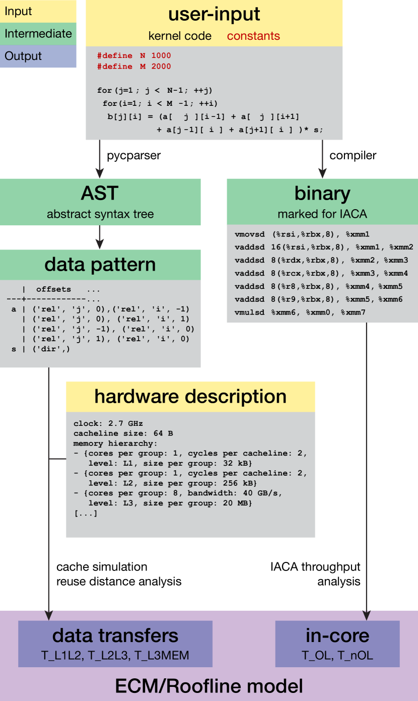
Figure 1: Overview of Kerncraft analysis

The ECM and Roofline analysis can be executed on any machine with the required software installed, since the code itself is not actually run. An optional “Benchmark” mode executes the compiled kernel code to measure the performance rather than predicting it, thereby validating the model(s).

In its current version the tool makes certain assumptions about the hardware and software that go beyond those required for the Roofline and ECM models: a perfect LRU cache replacement strategy and fully associative, fully inclusive, and write-allocate/write-back caches. These fit best to current Intel CPUs, but can be lifted to adapt the framework to other architectures. Furthermore, the compiler is assumed to not alter the data access characteristics of the “as-is” loop source code by, e.g., automatic blocking. Unless the tool is integrated in a compiler, this restriction is hard to circumvent.

Kerncraft and its support scripts are implemented in Python 2.7 and are available on the Python Package Index (PyPI).

4.2 Hardware description

The hardware description file contains information about the microarchitecture, the system architecture (e.g., number of cores and sockets), and microbenchmark results. It can be created by hand or with the help of the support script likwid_auto_bench.py, which automatically creates a formatted YAML [6] file by collecting the required information using likwid-topology and likwid-bench on the machine it is executed on. It performs microbenchmark runs with several streaming kernels in all memory hierarchy levels and with all possible numbers of cores and threads.

In addition to the automatically gathered information, cache transfer speeds, compiler flags, and the categorization of execution ports into overlapping and non-overlapping, among others, need to be manually added to the generated file.

Hardware information is required for all Kerncraft analyses, but it can be gathered beforehand, on the targeted machine, and reused for analysis runs on any other system. The hardware description files for the architectures used in this paper are distributed with the Kerncraft framework. Listing 2 contains the hardware description file for the Sandy Bridge machine described in Table 1, we left out the benchmark results and L2 and L3 cache descriptions for brevity.

Listing 2: Hardware description for Intel Xeon E5-2680 Sandy Bridge with 2 Sockets

⬇

clock: 2.7 GHz

cores per socket: 8

model type: Intel Core SandyBridge EP processor

model name: Intel Xeon CPU E5-2680 @ 2.70GHz

sockets: 2

threads per core: 2

cacheline size: 64 B

icc architecture flags: [-xAVX]

micro-architecture: SNB

FLOPs per cycle:

SP: {total: 16, ADD: 8, MUL: 8}

DP: {total: 8, ADD: 4, MUL: 4}

overlapping ports:

["0", "0DV", "1", "2", "3", "4", "5"]

non-overlapping ports: ["2D", "3D"]

memory hierarchy:

- {level: L1, cores per group: 1,

cycles per cacheline transfer: 2,

groups: 16, bandwidth: null,

size per group: 32.00 kB,

threads per group: 2}

# [... continues with description of L2 and L3]

- {level: MEM, cores per group: 8,

cycles per cacheline transfer: null,

groups: 1, bandwidth: null,

size per group: null,

threads per group: 16}

benchmarks:

kernels:

copy:

FLOPs per iteration: 0

read streams:

{bytes: 8.00 B, streams: 1}

read+write streams:

{bytes: 0.00 B, streams: 0}

write streams:

{bytes: 8.00 B, streams: 1}

# [... descriptions of daxpy, load, triad

# and update follow...]

measurements:

# [... bandwidth measurements follow ...]

4.3 Code input

Listing 3: 2D 5-point Jacobi kernel code

⬇

double a[M][N];

double b[M][N];

double s;

for(int j=1; j<M-1; ++j)

for(int i=1; i<N-1; ++i)

b[j][i] = (a[j][i-1] + a[j][i+1]

+a[j-1][i] + a[j+1][i]) * s;

}}}

The source code that is subject to the analysis must be provided in a separate file. The required syntax is based on the ISO C99 standard [13]. Constants (e.g., problem sizes) can be passed on the command line. To simplify the analysis, there are currently some restrictions on the full C99 standard. For instance, array declarations may only use fixed sizes or constants, with an optional addition or subtraction of an integer (e.g., double u[N][M+3][N-2][5], but not double u[M*N]), and array indices must use a loop index variable (with optional addition or subtraction), constants, or fixed integers. A full list of limitations may be found in the software documentation. Listing 3 shows a Jacobi kernel code with constants M and N defining the problem size in the two dimensions.

The pycparser [2] Python library is used for parsing the code. The resulting abstract syntax tree (AST) is then validated in regard to the mentioned restrictions and statically analyzed. We gather the following information: loop stack, data sources and destinations, and floating point operations (flop).

index variable	start	end	step size
j	1	499	+1
i	1	4999	+1

Table 2: Loop stack of Listing 3 with N=5000 and M=500

The loop stack contains information about all for loops in the code: their order, index variable name, start value, end value, and step size. See Table 2 for the loop stack information gathered from Listing 3.

variable	1st dimension	2nd dimension
a	relative $j$	relative $i-1$
	relative $j$	relative $i+1$
	relative $j-1$	relative $i$
	relative $j+1$	relative $i$
s	direct

Table 3: Data sources of Listing 3 with N=5000 and M=500

variable	1st dimension	2nd dimension
b	relative $j$	relative $i$

Table 4: Data destinations of Listing 3 with N=5000 and M=500

Data sources and destinations are retrieved from the statements in the innermost for loop. Any data access can be either direct (e.g., to a scalar or an array with constant or fixed index) or relative with an optional offset. Multidimensional arrays can have mixed accesses; for instance, xy[0][j][i+1] is a direct access on the first dimension, relative on the second, and relative with an offset of +1 on the third. See Tables 3 and 4 for the data access analysis of Listing 3.

Finally the floating point operation count of the inner loop body is extracted, for cases where a simple in-core model is required (e.g, if IACA is unavailable). Since this is based on the plain source code, compiler optimizations such as common subexpression elimination or compile-time evaluation, as well as more intricate dependencies on the in-core parallelism are ignored, and can lead to inaccuracies.

4.4 In-core prediction

We use the Intel Architecture Code Analyzer (IACA) to statically analyze the in-core performance of the kernel code. It is freely available and provides accurate throughput and critical path predictions for code execution under the assumption that all code and data comes from the L1 caches. Its predictions are based on documented as well as unreleased information about Intel CPUs from Nehalem to Haswell. The drawback is that older microarchitectures and architectures by other vendors are not supported.

IACA operates on binaries and therefore requires the code to be compiled. To do so, the kernel code is transformed by inserting it into a main function and adding boilerplate code to handle declarations and constants specified on the command line. All array declarations are replaced by pointer declarations with heap allocation using _mm_malloc in order to have arrays that are aligned to 32-byte boundaries. The use of heap memory prevents problems with stack size constraints. The loop stack is left untouched, but the inner loop’s statements are changed to reflect the changed declarations, by replacing multi-dimensional indexes with single-dimension index arithmetic. To prevent the compiler from eliminating parts of the benchmark code by optimization, calls to external dummy functions are inserted. The resulting code for the 2D-5pt Jacobi kernel is shown in Listing 4.

Listing 4: Runnable code (shortened) generated by Kerncraftfor IACA analysis with dummy function calls.

⬇

#include <stdlib.h>

void dummy(double *, ... );

extern int var_false;

int main(int argc, char **argv) {

const int N = atoi(argv[2]);

const int M = atoi(argv[1]);

double *a = _mm_malloc(

(sizeof(double)) * (M * N), 32);

for (int i=0; i<(M*N); ++i) a[i] = 0.23;

// [...] allocate and init b[]

double s = 0.23;

if (var_false) dummy(a, b, &s);

asm("nop"); // to limit search in assembly

for (int j=1; j<(M-1); ++j)

for (int i=1; i<(N-1); ++i)

b[i+(j*N)] = (a[(i-1)+(j*N)]

+ a[(i+1)+(j*N)]

+ a[i+((j-1)*N)]

+ a[i+((j+1)*N)]) * s;

asm("nop"); // to limit search in assembly

}

To narrow down the throughput analysis to the relevant loop section, IACA needs to find special markers in the machine code. These are inserted by our tool, modifying the assembly produced by the compiler. There is an option to insert markers as in-line assembly in the C source, but this interferes with compiler optimizations. Finding the correct block in the assembly code is done by selecting the block with the most vector instructions. The user can always fall back to an interactive procedure by providing a command line switch (--asm-block=manual) to Kerncraft.

The unrolling factor is extracted from the marked section by analyzing the loop counter increments used at the end of the selected block. This is needed to allow interpretation of the throughput analysis results from IACA. For example, if a loop is four times unrolled and IACA predicts a throughput of $32\,\mbox{cy}$ then one single loop iteration and update step takes $8\,\mbox{cy}$.

IACA provides the number of cycles, per execution port, that one unrolled iteration (i.e., one assembly code loop body) takes. In case of the 2D 5-point Jacobi kernel on a Sandy Bridge microarchitecture, it takes $16\,\mbox{cy}$ in the data portion of ports 2 and 3 (“2D” and “3D”). The maximum cycles of the data portions in ports 2 and 3 makes up the non-overlapping contribution, thus one might conclude that it would be 16 cy. However, one unrolled iteration encompasses two “work packages” (cache line lengths), so the applicable non-overlapping time is only $T_{\mathrm{nOL}}=8\,\mbox{cy}$. The specific port numbers that are responsible for non-overlapping execution are defined in the hardware description file.

The maximum cycles over all other ports make up the overlapping portion. It is $18\,\mbox{cy}$ with the code above on a Sandy Bridge microarchitecture, thus $T_{\mathrm{OL}}=9\,\mbox{cy}$.

4.5 Data traffic analysis

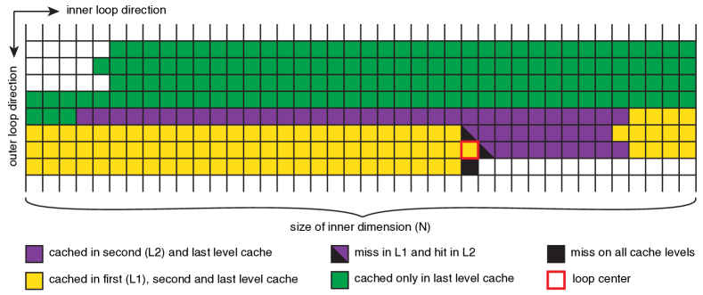
Figure 2: Cache usage prediction for the right-hand side array a[] on the 2D-5pt Jacobi kernel, with $N=40$ on a hypothetical machine with cache sizes that ensure the fulfillment of the layer condition in L3 and in L2, but not in the L1 cache.

The data traffic analysis is the central part of the Kerncraft tool, enabling most of the insight when analyzing streaming and stencil loop kernels. Its goal is to come up with predictions for the data volume from and into all memory hierarchy levels, so that the cycle counts required for the Roofline and ECM models can be determined. To this end we have implemented a simple “cache simulator” (see Sect. 4.1 above for the inherent assumptions about the hardware). In the following we explain its functionality using the 2D-5pt Jacobi example, since it is a basic but nontrivial case where temporal reuse of data is crucial for understanding performance properties.

Each cache level is inspected independently, although only misses in lower levels (closer to registers) are passed to the next higher level. We start off with all data requests from the loop iteration $i$, $j$ in the code from Listing 3 as shown in Tables 3 and 4: a[j-1][i], a[j][i-1], b[j][i], a[j][i+1], a[j+1][i]. Unfortunately, this notation does not offer any information about the actual location of the values in memory, so we change to a 1D-notation: a[(j-1)*N+i], a[j*N+i-1], b[j*N+i], a[j*N+i+1], a[(j+1)*N+i]. The mapping from 2D to 1D emphasizes the streaming nature of the data accesses, but without $N$, $i$, and $j$, it is still not sufficient. The inner problem size $N$ is specified by the user; we choose $N=40$ here. The indices $i$ and $j$ are kept abstract, but we assume a “loop center” at a relative offset of $0$ in either direction. If we plug this back into the 1D offsets, we are left with the following relative offsets: $-40$, $-1$, $0$, $+1$, $+40$.

We now start adding single iterations backwards in the indices $i$ and $j$ until the cache size is exceeded. After each addition of new offsets, they are checked for overlaps with the original set of accesses. If there is an overlap this is counted as a cache hit. Once the cache is full, it is easy to see that all offsets from the original set which were not turned into hits must be misses and thus contribute to cache or memory traffic. See Figure 2 for an illustration of all three cache levels. Note that, if there are many hits in the first level cache (L1), they are also hits in the second and last level, but since only misses lead to utilization of bandwidth, hits can be ignored. In our example we find one miss going all the way to memory: It is the first access to a new cache line in the outer loop direction (index $+40$, depicted in Fig. 2 as a black filled square). Also, there are two misses on L1 to the right of the loop center and above it, at offsets $-1$ and $+40$, but they are hits on L2. This situation can be expressed in terms of the “layer condition” [18]: Three consecutive layers of the grid fit into the L2 and L3 caches, but not into the L1 cache. However, the L1 cache is certainly large enough to ensure that all accesses to the left (index $-1$) will be L1 hits.

The actual communication between caches and memory is done in units of cache lines. Therefore the number of cache lines needs to be calculated from the offsets. We do not know any real memory address, so we arbitrarily decide that the first cache-line starts at offset $0$. Fig. 2 contains all information to predict data amounts originating from accesses to a[] between memory hierarchy levels: the all-black cell is a miss throughout all cache levels. The yellow cells are cached by L1 and therefore constitute traffic between registers and L1, which is encapsulated in $T_{\mathrm{nOL}}$ and given by IACA. The half-purple-half-black cells are misses in L1, but hits in L2 and therefore generate traffic between L1 and L2 and add to $T_{\mathrm{L1-L2}}$ with two cache lines. Since everything was already caught by higher cache levels, L3 has only the one original miss to handle. In order to take care of write-allocates, all writes offsets are also treated as reads. All write offsets are added to an evict list and no caching is tracked on this, meaning that all writes are immediately evicted as long as they go to offsets in arrays. In our example, this leads to an additional cache line transfer for each cache level.

4.6 Model construction

Kerncraft currently supports six analysis modes:

Roofline

Roofline with a simple in-core model based on arithmetic peak performance and L1 cache as an additional bandwidth bottleneck; does not require compiler or IACA

RooflineIACA

Roofline with IACA for in-core modeling

ECM

Full ECM model with IACA for in-core modeling

ECMData

Data transfer portion of ECM only; does not require compiler or IACA

ECMCPU

In-core (IACA-based) model only

Benchmark

Benchmark run for model validation

In the following we describe how the models in the first five modes are put together.

4.6.1 Roofline

The Roofline model can be constructed in two different ways, which are distinguished by the in-core modeling: either by using IACA (RooflineIACA mode) or by calculating the theoretical (MULT+ADD) arithmetic peak performance of the CPU (Roofline mode). If the theoretical peak is used, the L1 cache needs to be considered as another cache level and potential bandwidth bottleneck as described below. The peak performance is usually an over-optimistic estimate, because it assumes the perfect mix of operations, full SIMD vectorization, etc., for the given CPU. A more realistic model will replace this in future work.

Each memory level (except the L1 cache in RooflineIACA mode) is considered a potential data transfer bottleneck. As described in Sect. 2.2, cycle counts for the calculated data volume are determined based on microbenchmark results in the hardware description, giving a minimum execution time for every memory hierarchy level. Several microbenchmarks are available to provide a “closest match” to the actual loop code: e.g., if one read stream, one write stream, and one write-allocate stream hit a certain memory level, the measured bandwidth of an array copy benchmark in that level is used as the bandwidth baseline.

Among all lower execution time bounds for all memory levels and for the in-core execution, the largest is used as the Roofline model prediction (single-bottleneck view). Apart from the prediction in cycles per cache line, the tool also calculates the arithmetic intensity for the memory level that was found to be the bottleneck. For producing the output the cycle counts are by default converted to performance numbers in flop/s. This can be changed via a command line option (--unit cy/CL). In general, the units cy/CL, It/s, and FLOP/s can be selected.

4.6.2 ECM

The ECM analysis mode is split into two sub-modes: ECMData for the data access and cache analysis, and ECMCPU for the in-core analysis performed by IACA. The model ECM combines both submodels and gives an overall prediction. The reason for the split is that IACA may not be available on all systems, and it does not support microarchitectures other than Intel’s. In such cases one may still use the ECMData model to get the data traffic analysis.

Using the in-core prediction and the transfer times between adjacent cache levels, the ECM model is put together and printed using the syntax as described in Sect. 2.3. By default the report is in cy/CL, but the standard options (see the previous section) are available to change this. The tool also reports the number of cores at which the performance is expected to saturate.

Examples for the application and the output of the tool can be found in Sect. 5 below.

4.7 Model validation (Benchmark mode)

The Benchmark mode of Kerncraft does not predict performance but measures it. Therefore this mode must be executed on the same machine as described in the hardware description file. A matching hardware description is necessary to determine the appropriate compiler flags, cache line sizes, and clock speed. For the measurement results to be generated correctly, the user must fix the CPU frequency to the clock speed defined in the machine file.

In order to allow execution of the kernel code, it is transformed in a similar manner as for IACA, described in Section 4.4, but with one extra for loop inserted that wraps all kernel loops. This is to prolong the total execution time for improved accuracy with small problem sizes. Also, calls to the LIKWID marker application programming interface are inserted before and after the outer for loop for a precise measurement of the loop section only, without overhead from allocating and initializing memory. After successful transformation and compilation, the binary is executed with likwid-perfctr, LIKWID’s performance counter and pinning command. Proper thread-core affinity is therefore ensured. The marker calls can also be used for advanced validation using data volume, cycles per instruction, and work-related metrics, but this feature is not leveraged in the current version of Kerncraft. The runtime is used to calculate the number of cycles per work unit.

5 Evaluation

Here we evaluate the correctness of predictions derived by Kerncraft from kernel codes and hardware descriptions. It is out of the scope of this work to evaluate the underlying performance models; this has been discussed elsewhere [4, 23, 8, 18, 11, 10]. We will, however, compare predictions by Kerncraft to predictions derived by manual analysis in previously published papers (see Table 5) and point out relevant differences and peculiarities. We only consider predictions for serial code on in-memory data sets here, although both models are certainly capable of providing in-cache and multi-threaded results as well (supported by the --cores option). The same binary code has been produced for the Sandy Bridge and the Haswell CPU, but IACA was run with the appropriate architectural setting.

			Kerncraft					Reference
			Const.	ECM Model	ECM	Roofline1	Bench.	ECM Model	Roofline1
Kernel	Code	Arch.	$N$	(cy/CL)	(cy/CL)	(cy/CL)	(cy/CL)	(cy/CL)	(cy/CL)
2D-5pt	List. 3	SNB	$6000$	$\left\{{9.5}\,\|\,{8}\,|\,{10}\,|\,{6}\,|\,{12.7}\right\}\,{}$	$36.7$	$29.8$	$36.4$	$\left\{{6}\,\|\,{8}\,|\,{10}\,|\,{10}\,|\,{13}\right\}\,{}$ [18]	n/a
		HSW		$\left\{{9.4}\,\|\,{8}\,|\,{5}\,|\,{6}\,|\,{16.7}\right\}\,{}$	$35.7$	$26.6$	$30.0$	n/a	n/a
UXX	List. 6	SNB	$150$	$\left\{{84}\,\|\,{32.5}\,|\,{20}\,|\,{20}\,|\,{26.3}\right\}\,{}$	$98.8$	$84.0$	$112.5$	$\left\{{84}\,\|\,{38}\,|\,{20}\,|\,{20}\,|\,{26}\right\}\,{}$ [18]	n/a
		HSW		$\left\{{56}\,\|\,{27.5}\,|\,{10}\,|\,{20}\,|\,{31.6}\right\}\,{}$	$89.1$	$61.7$	$86.9$	n/a	n/a
long-range	List. 7	SNB	$100$	$\left\{{57}\,\|\,{53}\,|\,{24}\,|\,{24}\,|\,{17.0}\right\}\,{}$	$118.0$	$65.9$	$134.2$	$\left\{{68}\,\|\,{64}\,|\,{24}\,|\,{24}\,|\,{17}\right\}\,{}$ [18]	n/a
		HSW		$\left\{{57}\,\|\,{47.5}\,|\,{12}\,|\,{24}\,|\,{22.3}\right\}\,{}$	$105.8$	$63.6$	$104.5$	n/a	n/a
Kahan-dot	List. 8	SNB		$\left\{{96}\,\|\,{8}\,|\,{4}\,|\,{4}\,|\,{7.8}\right\}\,{}$	$96.0$	$96.0$	$101.1$	$\left\{{32}\,\|\,{8}\,|\,{4}\,|\,{4}\,|\,{7.9}\right\}\,{}$ [11]	n/a
		HSW		$\left\{{96}\,\|\,{8}\,|\,{2}\,|\,{4}\,|\,{9.1}\right\}\,{}$	$96.0$	$96.0$	$98.0$	n/a	n/a
Schönauer	List. 9	SNB		$\left\{{4}\,\|\,{6}\,|\,{10}\,|\,{10}\,|\,{21.9}\right\}\,{}$	$47.9$	$54.3$	$58.8$	$\left\{{4}\,\|\,{6}\,|\,{10}\,|\,{10}\,|\,{24}\right\}\,{}$ [8]	n/a
Triad		HSW		$\left\{{4}\,\|\,{3}\,|\,{5}\,|\,{10}\,|\,{26.3}\right\}\,{}$	$44.3$	$46.4$	$48.3$	n/a	n/a

Table 5: Single-thread Kerncraft predictions for five benchmark kernels in comparison to reference predictions from previous publications.

5.1 Stencil Codes

We choose three interesting “corner case” stencils that have been comprehensively analyzed in [18] using the ECM model on a Sandy Bridge base microarchitecture: 2D-5pt Jacobi, UXX, and a fourth-order long-range stencil.

5.1.1 2D-5pt Jacobi

Listing 5: Kerncraft output for the analysis of the 2D-5pt Jacobi kernel on the Sandy Bridge microarchitecture (node name “phinally”) with $N=6000$ and $M=6000$ (output adapted for brevity)

⬇

1$ kerncraft -p ECM --cores 1 \

-m machine-files/phinally.yaml \

3 kernels/2d-5pt.c \

-D N 6000 -D M 6000

5

saturating at 3 cores

7

$ kerncraft -p RooflineIACA\

9 --unit cy/CL --cores 1 \

-m machine-files/phinally.yaml \

11 kernels/2d-5pt.c \

-D N 6000 -D M 6000 -v

13

Bottlnecks:

15 level | ar.int. | perfor. | bandw. | bw kernel

| FLOP/b | cy/CL | GB/s |

17-------+---------+---------+--------+----------

CPU | | 9.5 | |

19 L1-L2 | 0.1 | 16.9 | 51.2 | triad

L2-L3 | 0.1 | 27.5 | 31.5 | triad

21L3-MEM | 0.17 | 29.8 | 17.4 | copy

23Cache or mem bound

(bw with from copy benchmark)

25Arithmetic Intensity: 0.17 FLOP/b

In Listing 5 we show the Kerncraft command line arguments and generated output for the 2D 5-point Jacobi stencil (Listing 3) for Sandy Bridge. In line number LABEL:l:ecm we see the ECM model and line number LABEL:l:ecmp shows the ECM prediction notation. The results in Table 5 have a difference of $3\,\mbox{cy}$ in $T_{\mathrm{OL}}$ on Sandy Bridge compared to the analysis in [18]. This is due to the compiler using half-wide (16-byte) load instructions in our case. The half-wide loads take the same number of cycles as full-wide loads, but require two addresses to be generated. In combination with an additional address required for full-width store operations, this leads to an average of $9\,\mbox{cy}$ of address generation per cache-line. The same happens on Haswell, although it has one additional address generation unit. However, this unit can only be utilized with simple addressing modes, and the compiler does not leverage this feature. On Haswell the ECM model is outperformed by the measurement by almost 20%. This is very unusual, although the model is not strictly optimistic like Roofline, and will be investigated.

The Roofline model is much more optimistic than the ECM model for this code, since the memory bottleneck does not dominate the single-core execution time: The layer condition can only be satisfied in the L2 cache for the chosen inner problem size ($N=6000$). If spatial blocking for the L1 cache is performed (or if the inner loop size is short enough), Roofline becomes more accurate as shown in [18].

5.1.2 UXX (double precision)

Listing 6: Kernel code for the UXX stencil in double precision

⬇

double u1[M][N][N], d1[M][N][N], xx[M][N][N];

double xy[M][N][N], xz[M][N][N], c1,c2,d,dth;

for(int k=2; k<M-2; k++) {

for(int j=2; j<N-2; j++) {

for(int i=2; i<N-2; i++) {

d = (d1[k-1][j][i] + d1[k-1][j-1][i]

+ d1[k][j][i] + d1[k][j-1][i])*0.25;

u1[k][j][i] = u1[k][j][i] + (dth/d)

* ( c1*(xx[k][j][i] - xx[k][j][i-1])

+ c2*(xx[k][j][i+1] - xx[k][j][i-2])

+ c1*(xy[k][j+1][i] - xy[k][j-1][i])

+ c2*(xy[k][j+1][i] - xy[k][j-2][i])

+ c1*(xz[k][j][i] - xz[k-1][j][i])

+ c2*(xz[k+1][j][i] - xz[k-2][j][i]));

}}}

The UXX stencil (Listing 6) has a long-latency divide operation in the inner loop that cannot be easily avoided and that dominates the overlapping time. This explains the large difference between Sandy Bridge and Haswell in terms of $T_{\mathrm{OL}}$. The discrepancy in $T_{\mathrm{nOL}}$ compared to the reference result is due to the more current compiler, but there is also a deviation between Haswell and Sandy Bridge: The compiler generates a mixture of full-wide (32-byte) and half-wide (16-byte) load instructions. Since both architectures can execute two half-wide loads per cycle, but only Haswell can do two full-wide loads per cycle, Haswell has a slight advantage in load throughput and, consequently, in $T_{\mathrm{nOL}}$.

5.1.3 Long-range

Listing 7: Kernel code for the long-range stencil

⬇

double U[M][N][N], V[M][N][N], ROC[M][N][N];

double c0, c1, c2, c3, c4, lap;

for(int k=4; k < M-4; k++) {

for(int j=4; j < N-4; j++) {

for(int i=4; i < N-4; i++) {

lap = c0*V[k][j][i]

+ c1*(V[k][j][i+1] + V[k][j][i-1])

+ c1*(V[k][j+1][i] + V[k][j-1][i])

+ c1*(V[k+1][j][i] + V[k-1][j][i])

+ c2*(V[k][j][i+2] + V[k][j][i-2])

+ c2*(V[k][j+2][i] + V[k][j-2][i])

+ c2*(V[k+2][j][i] + V[k-2][j][i])

+ c3*(V[k][j][i+3] + V[k][j][i-3])

+ c3*(V[k][j+3][i] + V[k][j-3][i])

+ c3*(V[k+3][j][i] + V[k-3][j][i])

+ c4*(V[k][j][i+4] + V[k][j][i-4])

+ c4*(V[k][j+4][i] + V[k][j-4][i])

+ c4*(V[k+4][j][i] + V[k-4][j][i]);

U[k][j][i] = 2.f*V[k][j][i] - U[k][j][i]

+ ROC[k][j][i] * lap; }}}

The fourth-order long-range stencil (Listing 7) shows a very low fraction of execution time in $T_{\mathrm{L3Mem}}$ due to a massive amount of data (layers) that have to be supplied by the caches. The results in Table 5 exhibit a slight deviation in $T_{\mathrm{OL}}$ of $16\,\mbox{cy}$ and in $T_{\mathrm{nOL}}$ of $9\,\mbox{cy}$ on Sandy Bridge compared to published results. The lower cycle predictions in our analysis can be attributed to better compiler-generated code (fewer register spills). Again, Haswell has a slight advantage over Sandy Bridge in terms of $T_{\mathrm{nOL}}$ cycles due to the compiler partially producing full-wide load instructions. The Roofline prediction is massively over-optimistic in all cases since it assumes a core-bound situation, whereas in fact the execution time is spread almost evenly between in-core and data transfer contributions.

The long-range stencil constitutes an instructive example for demonstrating the complicated situations that can arise with stencil codes on architectures with multiple caches.

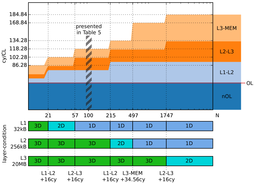
Figure 3: Top: Single-core ECM model predictions for the 3D long-range stencil (Listing 7) with increasing inner (and middle) dimension $N$ and a memory-bound data set. Bottom: Visualization of fulfilled layer conditions in the three cache levels. A 3D/2D/1D layer condition pertains to loop index $k$, $j$, and $i$, respectively.

In Fig. 3 we show graphically the contributions to the ECM model in cycles per cache line versus the inner and middle loop size (both set to $N$). The entry in Table 5 uses $N=100$ (marked in the figure). Varying $N$ leads to layer conditions being fulfilled and violated in different cache levels; overall, six situations can be distinguished over the $N$ range considered, shown at the bottom of the figure: for instance, around $N\approx 1000$ the layer condition in the outer ($k$) dimension is met in the L3 cache alone, whereas the L2 and L1 caches are too small to even hold a sufficient number of rows to meet the layer condition in the middle ($j$) dimension.

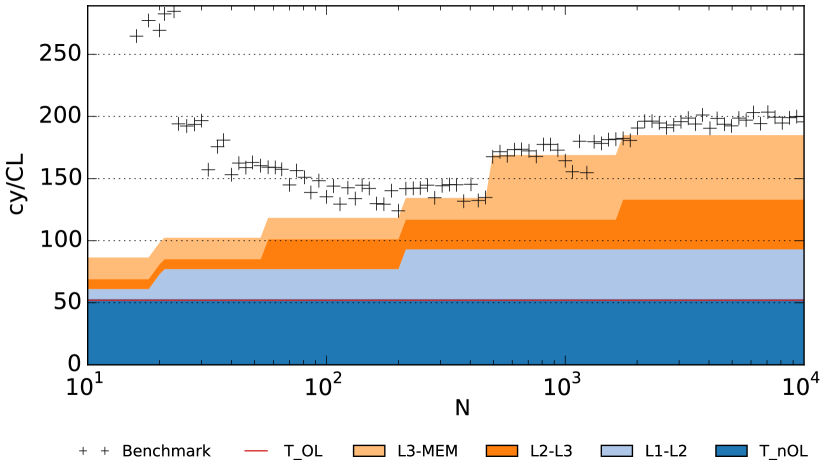
Figure 4: Validation of the single-core ECM prediction for the 3D long-range stencil (as presented in Fig. 3), with measurements (crosses) on SNB.

Figure 4 shows the predictions together with measured data (crosses). The general behavior with increasing $N$ is well tracked by the model starting at $N\gtrsim 200$, but there are considerable deviations for smaller $N$. This is expected since the steady-state assumption cannot be upheld with short inner loops, and boundary effects become non-negligible.

5.2 Streaming Kernels

Kerncraft does not only support the analysis of stencil codes, but also accepts typical streaming kernels found in numerical vector arithmetic and memory benchmarks. Here we will have a look at the Kahan-compensated double-precision dot product and the Schönauer Triad. These have been analyzed thoroughly in [11] and [8], respectively.

Listing 8: Kernel code for Kahan-ddot

⬇

double a[N], b[N], c;

double sum, prod, t, y;

for(int i=0; i<N; ++i) {

prod = a[i] * b[i]; y = prod - c;

t = sum + y; c = (t - sum) - y; sum = t;

}

5.2.1 Kahan-ddot

The code is shown in Listing 8. It provides a scalar product of two arrays a[] and b[], correcting for round-off errors due to the finite-precision floating-point number representation [14]. As was shown in [11], current compilers fail in generating efficient (or correct) machine code from the C source. In our case the compiler could not use SIMD vectorization due to the presence of a loop-carried dependency, but it produced correct scalar code without further unrolling. As a consequence the runtime is dominated by the loop-carried dependency and IACA reports $T_{\mathrm{OL}}=96\,\mbox{cy/CL}$ even in throughput mode. Here we find a case where the ECM and Roofline predictions coincide due to the strong dominance of $T_{\mathrm{OL}}$.

The result for $T_{\mathrm{nOL}}$ on Sandy Bridge in Table 5 differs from the reference result, since the latter was produced with a scalar but otherwise optimal version of the code that used modulo unrolling to hide the inter-iteration stalls. Note also that [11] uses latency penalties to make the ECM model work better in memory. The Kerncraft tool has this capability (in fact, the penalty cycles are part of the machine files), but it is deactivated by default.

5.2.2 Schönauer Triad

The Schönauer Triad (Listing 9) is a simple streaming kernel which is designed to be limited by data transfers on all processor architectures even if the data resides in the innermost cache.

The deviation of $T_{\mathrm{L3-MEM}}$ compared to the reference results in Table 5 on Sandy Bridge is due to the application of a slightly different peak memory bandwidth. It is striking that the ECM model is more optimistic than Roofline for this benchmark, but this only shows that the latter is based on a measured bandwidth value (with the very same microbenchmark kernel); on the other hand it is known that the ECM model is slightly optimistic with very tight, data-bound kernels, presumably because of hardware prefetchers not keeping up with the in-core execution in this case. Since the model assumes perfect prefetching, this deviation could be fixed by adding latency penalty cycles to the single-core execution.

Listing 9: Kernel code for the Schönauer Triad

⬇

double a[N], b[N], c[N], d[N], s;

for(int i=0; i<N; ++i)

a[i] = b[i] + c[i] * d[i];

6 Related Work

There are many performance modeling tools that rely on hardware metrics, statistical methods, curve fitting, and machine learning, but there are currently only four projects in the area of automatic analytic modeling that we know of: PBound, ExaSAT, Roofline Model Toolkit and MAQAO.

Narayanan et al. [15] describe a tool (PBound) for automatically extracting relevant information about execution resources (arithmetic operations, loads and stores) from source code. They do not, however, consider cache effects and parallel execution, and their machine model is rather idealized. Unat et al. [22] introduce the ExaSAT tool, which uses compiler technology for source code analysis. They also employ “layer conditions” [18] to assess the real data traffic for every memory hierarchy level based on cache and problem sizes. They use an abstract simplified machine model, whereas our Kerncraft tool employs Intel IACA (see Sect. 2.1) to generate more accurate in-core predictions. On the one hand this restricts Kerncraft in-core predictions to Intel CPUs, but on the other hand provides predictions from the actual machine code containing all the optimizations provided by the compiler. Furthermore, ExaSAT is restricted to the Roofline model for performance prediction. On the other hand, being compiler-based, ExaSAT supports full-application modeling and code optimizations, which is out of scope in the current version of Kerncraft. It can also incorporate communication (i.e., message passing) overhead. Lo et al. [17] have recently introduced the “Roofline Model Toolkit,” which aims at automatically generating hardware descriptions for Roofline analysis. They do not support automatic topology detection, however, and their use of compiler-generated loops introduces an element of uncertainty. Djoudi et al. [5] started the MAQAO Project in 2005, which uses static analysis to predict in-core execution time and combines it with dynamic analysis to assess the overall code quality. It was originally developed for the Itanium 2 but has since been adapted for recent Intel64 architectures and the Xeon Phi. As with Kerncraft, MAQAO currently supports only Intel architectures. The memory access analysis is based on dynamic run-time data, i.e., it requires the code to be run on the target architecture.

There is to our knowledge no tool comparable to IACA for non-Intel CPUs. Fallback support for in-core predictions based on automatic code analysis and architectural information (as done, e.g., in [22]) is work in progress.

7 Summary and Outlook

The power and utility of analytic performance modeling is undisputed, but the construction of accurate models is a tedious task that requires considerable time and experience. The Kerncraft tool enables analytic (Roofline or ECM) modeling of loop kernels on modern CPU architectures under well-defined conditions. We have shown that predictions generated by Kerncraft concur with published numbers on a variety of codes and two modern Intel architectures. However, it must be emphasized that Kerncraft is not a “black-box” tool that can be applied blindly without background knowledge. In contrast, it is the deviation of generated models from experience or from measured results that sparks new insight. This is impossible without a basic understanding about the software and the capabilities of the hardware it is running on.

Currently the applicability of the tool is restricted by dependencies on the Intel-specific IACA tool and compilers. But even without those Kerncraft can still predict data locality and cache behavior. Since the basic principles of the modeling process implemented in Kerncraft are widely applicable, support for other architectures is a matter of extending the ECM model appropriately. Currently we are working on adapting the model to ARM-based chips. To further enhance the tool in the short term we will support single precision floating-point numbers, passing pragma directives to the compiler, and allowing for other compilers than ICC. On the ECM model side, non-inclusive cache hierarchies and non-temporal stores need further evaluation but will be implemented as well. It will be a more difficult task to find or build a suitable replacement for IACA and to predict the data transfer properties of non-contiguous access patterns. The simplistic cache model in Kerncraft may be extended to non-LRU cache replacement policies and non-fully associative caches, but we consider such additions less crucial.

To combine dynamic analysis with performance modeling, we plan to introduce phenomenological models where data traffic and bandwidth measurements are used to improve the validation procedure and to capture effects that can not be easily modeled, such as irregular memory accesses as found, e.g., in sparse-matrix algorithms. The required infrastructure to take the necessary data is already functional in the current version of Kerncraft.

References

- [1] Kerncraft toolkit. https://github.com/RRZE-HPC/kerncraft.
- [2] E. Bendersky. pycparser. https://github.com/eliben/pycparser.
- [3] D. Callahan, J. Cocke, and K. Kennedy. Estimating interlock and improving balance for pipelined architectures. Journal of Parallel and Distributed Computing, 5(4):334 – 358, 1988. DOI: 10.1016/0743-7315(88)90002-0.
- [4] K. Datta, S. Kamil, S. Williams, L. Oliker, J. Shalf, and K. Yelick. Optimization and performance modeling of stencil computations on modern microprocessors. SIAM Review, 51(1):129–159, 2009.
- [5] L. Djoudi, D. Barthou, P. Carribault, C. Lemuet, J.-T. Acquaviva, W. Jalby, et al. MAQAO: Modular assembler quality analyzer and optimizer for itanium 2. In The 4th Workshop on EPIC architectures and compiler technology, San Jose, 2005. http://www.prism.uvsq.fr/users/bad/Research/ps/maqao.pdf.
- [6] C. Evans, B. Ingerson, and O. Ben-Kiki. YAML Ain’t Markup Language. http://yaml.org.
- [7] D. Hackenberg, R. Schöne, T. Ilsche, D. Molka, J. Schuchart, and R. Geyer. An energy efficiency feature survey of the Intel Haswell processor. In Workshop on High-Performance, Power-Aware Computing (HPPAC) 2015. Accepted for publication.
- [8] G. Hager, J. Treibig, J. Habich, and G. Wellein. Exploring performance and power properties of modern multi-core chips via simple machine models. Concurrency and Computation: Practice and Experience, pages n/a–n/a, 2014. DOI:10.1002/cpe.3180.
- [9] R. W. Hockney and I. J. Curington. : A parameter to characterize memory and communication bottlenecks. Parallel Computing, 10(3):277–286, 1989. DOI: 10.1016/0167-8191(89)90100-2.
- [10] J. Hofmann, J. Eitzinger, and D. Fey. Execution-cache-memory performance model: Introduction and validation. Technical report, Chair for Computer Architecture, University of Erlangen-Nuremberg, 2015. http://arxiv.org/abs/1509.03118.
- [11] J. Hofmann, D. Fey, J. Eitzinger, G. Hager, and G. Wellein. Performance analysis of the Kahan-enhanced scalar product on current multicore processors. CoRR, abs/1505.02586, 2015. Accepted for PPAM’2015, the 11th International Conference on Parallel Processing and Applied Mathematics, September 6-9, 2015, Krakow, Poland, http://arxiv.org/abs/1505.02586.
- [12] Intel Architecture Code Analyzer. https://software.intel.com/en-us/articles/intel-architecture-code-analyzer.
- [13] ISO. ISO C Standard 1999. Technical report, 1999. ISO/IEC 9899:1999 draft.
- [14] W. Kahan. Pracniques: Further remarks on reducing truncation errors. Commun. ACM, 8(1), Jan. 1965.
- [15] S. H. Krishna Narayanan, B. Norris, and P. D. Hovland. Generating performance bounds from source code. In Parallel Processing Workshops (ICPPW), 2010 39th International Conference on, pages 197–206, Sept 2010. DOI: 10.1109/ICPPW.2010.37.
- [16] H. T. Kung. Memory requirements for balanced computer architectures. In Proceedings of the 13th Annual International Symposium on Computer Architecture, ISCA ’86, pages 49–54, Los Alamitos, CA, USA, 1986. IEEE Computer Society Press. DOI: 10.1145/17356.17362.
- [17] Y. Lo, S. Williams, B. Van Straalen, T. Ligocki, M. Cordery, N. Wright, M. Hall, and L. Oliker. Roofline model toolkit: A practical tool for architectural and program analysis. In S. A. Jarvis, S. A. Wright, and S. D. Hammond, editors, High Performance Computing Systems. Performance Modeling, Benchmarking, and Simulation, volume 8966 of Lecture Notes in Computer Science, pages 129–148. Springer International Publishing, 2015. DOI: 10.1007/978-3-319-17248-4_7.
- [18] H. Stengel, J. Treibig, G. Hager, and G. Wellein. Quantifying performance bottlenecks of stencil computations using the execution-cache-memory model. In Proceedings of the 29th ACM International Conference on Supercomputing, ICS ’15, pages 207–216, New York, NY, USA, 2015. ACM. DOI: 10.1145/2751205.2751240.
- [19] J. Treibig, G. Hager, and G. Wellein. LIKWID: A lightweight performance-oriented tool suite for x86 multicore environments. 2012 41st International Conference on Parallel Processing Workshops, 0:207–216, 2010. DOI: 10.1109/ICPPW.2010.38.
- [20] J. Treibig, G. Hager, and G. Wellein. likwid-bench: An extensible microbenchmarking platform for x86 multicore compute nodes. In H. Brunst, M. S. Müller, W. E. Nagel, and M. M. Resch, editors, Tools for High Performance Computing 2011, pages 27–36. Springer Berlin Heidelberg, 2012. DOI: 10.1007/978-3-642-31476-6_3.
- [21] J. Treibig, G. Hager, and G. Wellein. Performance patterns and hardware metrics on modern multicore processors: Best practices for performance engineering. In I. Caragiannis, M. Alexander, R. Badia, M. Cannataro, A. Costan, M. Danelutto, F. Desprez, B. Krammer, J. Sahuquillo, S. Scott, and J. Weidendorfer, editors, Euro-Par 2012: Parallel Processing Workshops, volume 7640 of Lecture Notes in Computer Science, pages 451–460. Springer Berlin Heidelberg, 2013.
- [22] D. Unat, C. Chan, W. Zhang, S. Williams, J. Bachan, J. Bell, and J. Shalf. ExaSAT: An exascale co-design tool for performance modeling. International Journal of High Performance Computing Applications, 29(2):209–232, 2015. DOI: 10.1177/1094342014568690.
- [23] S. Williams, A. Waterman, and D. Patterson. Roofline: An insightful visual performance model for multicore architectures. Commun. ACM, 52(4):65–76, 2009. DOI: 10.1145/1498765.1498785.