Fundamental Groups of a Class of Rational Cuspidal Plane Curves

Abstract

We compute the presentations of fundamental groups of the complements of a class of rational cuspidal projective plane curves classified by Flenner, Zaidenberg, Fenske and Saito. We use the Zariski-Van Kampen algorithm and exploit the Cremona transformations used in the construction of these curves. We simplify and study these group presentations so obtained and determine if they are abelian, finite or big, i.e. if they contain free non-abelian subgroups. We also study the quotients of these groups to some extend.

1 Introduction

A projective plane curve $C\subset\mathbb{P}^{2}$ is said to be cuspidal if all its singularities are irreducible. It is said to be of type $(d,m)$ if $C$ is of degree $d$ and the maximal multiplicity of its singularities is $m$, i.e. $m=\max_{p\in C}(\mbox{mult}_{p}C)$. Rational cuspidal curves of type $(d,d-2)$ and those of type $(d,d-3)$, having at least three cusps has been classified by Flenner and Zaidenberg. It turns out that these curves have exactly three cusps, moreover, the rational 3-cuspidal curves of type $(d,d-2)$ can be obtained from the quadric $\{xy-z^{2}=0\}$, and the rational 3-cuspidal curves of type $(d,d-3)$ can be obtained from the cubic $\{xy^{2}-z^{3}=0\}$ by means of Cremona transformations. Our aim in this paper is to compute the fundamental groups of complements of these curves as well as those ones constructed in the ensuing work of Fenske, Sakai and Tono.

Given an algebraic curve $C\subset\mathbb{P}^{2}$, it is interesting to study the topology of its complement $\mathbb{P}^{2}\backslash C$ from the point of view of the classification theory of algebraic curves. The idea is an analogue of the leading principle in the knot theory: in order to understand a knot ${\cal K}\subset S^{3}$, look at the topology of the knot complement $S^{3}\backslash{\cal K}$. Another strong motivation for studying $\pi_{1}(\mathbb{P}^{2}\backslash C)$ comes from the surface theory: A good knowledge of $\pi_{1}(\mathbb{P}^{2}\backslash C)$ allows one to construct Galois coverings of $\mathbb{P}^{2}$ branched at $C$ (see [12] for explicit examples). Moreover, if $X\rightarrow\mathbb{P}^{2}$ is a branched covering, with $C$ as the branching locus, one can hope to derive some invariants of $X$ from the invariants of the topology of $\mathbb{P}^{2}\backslash C$. The study of $\pi_{1}(\mathbb{P}^{2}\backslash C)$ has been initiated by Zariski in the thirties [13]. Although the prevailing convention in the literature is to call $\pi_{1}(\mathbb{P}^{2}\backslash C)$, by abuse of language, the fundamental group of $C$, following Degtyarev [2], we shall take the liberty to call it simply the group of $C$. Degtyarev classified the possible groups of curves of degree $d$ with a singular point of multiplicity $d-2$ and calculated the groups of all quintics (irreducible or not). Hence, groups of curves of degree $\leq 5$ are known. This is not the case starting with the sextics. A special class of sextics, namely the rational cuspidal ones, has been classified by Fenske [4], see Theorem 2.7. Their groups are given in Corollary 2.4.

Below we review these classification results followed by Artal’s and our results on the fundamental groups. Since group computations uses the explicit construction of these curves, we felt obliged to give a detailed account of classification results.

Acknowledgements.

These results are from authors’s thesis. Hereby I express my gratitude towards M. Zaidenberg who suggested the problem. I am indebted to Alex Dimca for informing that they are useful and referred, and for his encouragement to publish them. I am thankful to Hakan Ayral for his help with the graphics.

2 Classifications and fundamental groups

We use the following conventions settled in [7]: the multiplicity sequence of a cusp will be called the type of this cusp. Recall that if

$$V_{n+1}\rightarrow V_{n}\rightarrow\cdots V_{1}\rightarrow V_{0}=\mathbb{C}^{2}$$

is a minimal resolution of an irreducible analytic curve singularity germ $(C,0)\subset(\mathbb{C}^{2},0)$, and $(C_{i},P_{i})$ denotes the proper transform of $(C,0)$ in $V_{i}$, so that $(C_{0},P_{0})=(C,O)$, then the sequence

$$[m^{(n+1)},m^{(n)},\dots,m^{(1)},m^{(0)}]$$

, where $m^{(i)}:={\rm mult}_{P_{i}}C_{i}$, is called the multiplicity sequence of $(C,0)$. Evidently, $m^{(i+1)}\leq m^{(i)}$, $m^{(n)}\geq 2$, and $m^{(n+1)}=1$. The (sub)sequence

$$\underbrace{k,k,k,\dots,k}_{m\;\scriptsize{\mbox{times}}}$$

will be abbreviated by $k_{m}$. For instance, $[kn,k_{n+m},k-1]$ is the sequence $[kn,\underbrace{k,k,k,\dots,k}_{n+m\;\scriptsize{\mbox{times}}},k-1]$. Also, the last term of the multiplicity sequence will be omitted. Under this notation, $[2]$ corresponds to a simple cusp and $[2_{3}]=[2,2,2]$ corresponds to a ramphoid cusp.

Theorem 2.1.

(Flenner-Zaidenberg [6]) A rational cuspidal curve of type $(d,d-2)$ with at least three cusps has exactly three cusps. For each $(d,n,m)\in\mathbb{N}^{3}$ such that $d\geq 4$, $n\geq m>0$ and $n+m=d-2$ there is exactly one (up to projective equivalence) such curve $C$, whose cusps are of types $[d-2]$, $[2_{n}]$, $[2,2_{m}]$. There are no other rational cuspidal curves of type $(d,d-2)$ with number of cusps $\geq 3$.

Note that an irreducible curve of type $(d,d-1)$ is rational, and has an abelian group by a classical computation due to Zariski.

Theorem 2.2.

(Artal [1]) Let $C$ be as in Theorem 2.1. Then the group of $C$ admits the presentation

$$\pi_{1}(\mathbb{P}^{2}\backslash C)=\langle a,b\,|\,(ba)^{d-1}=b^{d-2},\quad(ba)^{k}b=a(ba)^{k}\rangle,$$

where $k\geq 0$ and $2k+1={\rm gcd}(2n+1,\,2m+1)$. Hence, the group depends only on $(d,k)$. This group is abelian if and only if $k=0$, finite of order $12$ if $(d,n,m)=(4,1,1)$, finite of order $840$ if $(d,n,m)=(7,4,1)$, otherwise it is a big group .

Note that the case $(d,n,m)=(4,1,1)$ corresponds to the three cuspidal quartic, whose group had been calculated already by Zariski [13].

Taking for example $C_{1}$ with $(d,n,m)=(13,10,1)$ and $C_{2}$ with $(d,n,m)=(13,7,4)$, one has the following result.

Corollary 2.1.

(Artal [1]) There exist infinitely many pairs $(C_{1},C_{2})$ of curves with isomorphic (big) groups, but different homeomorphism types of the pairs $(\mathbb{P}^{2},C_{1})$, $(\mathbb{P}^{2},C_{2})$.

Theorem 2.3.

(Flenner-Zaidenberg [7]) A rational cuspidal curve of type $(d,d-3)$ with at least three cusps has exactly three cusps. For each $d=2n+3$, $n\geq 1$, there is exactly one (up to projective equivalence) such curve $C_{n}$, and the cusps of $C_{n}$ are of types $[2n,2_{n}]$, $[3_{n}]$, $[2]$. There are no other rational cuspidal curves of type $(d,d-2)$ with number of cusps $\geq 3$.

Theorem 2.4.

Let $C_{n}$ be as in Theorem 2.3, where $d=2n+3$. Then the group of $C_{n}$ admits the presentation

$$\pi_{1}(\mathbb{P}^{2}\backslash C_{n})=\langle c,b\,|\,cbc=bcb,\quad b^{n}c^{n+2}=c^{n+2}b^{n},\quad(b^{-n}cb^{2})^{n+1}c^{n^{2}}=1\rangle.$$

This group is big when $n$ is odd and $\geq 7$, abelian when $n\in\{0,1,2\}$, and finite of order $8640$ for $n=3$, and finite of order 1560 for $n=5$.

This is proved in 3.3.1 below.

These classification results have been completed (independently) in the works of Fenske and Sakai-Tono:

Theorem 2.5.

(Fenske [4], Sakai-Tono [11]) Let $n,m\in\mathbb{N}$ be such that $n\geq 1$ and $0\leq m<n$.
(i) A rational cuspidal curve of type $(d,d-2)$ with exactly one cusp exists if and only if $d=2n+2$. Such a curve is unique up to projective equivalence, and the type of its cusp is $[2n,2_{2n}]$.
(ii) A rational cuspidal curve of type $(d,d-2)$ with exactly two cusp exists if and only if
(a) $d=2n+3$, with types of cusps $[2n+1,2_{n}]$, $[2_{n+1}]$;
(b) $d=n+2$, with types of cusps $[n]$, $[2_{n}]$;
(c) $d=2n+2$, with types of cusps $[2n,2_{n+m}]$, $[2_{n-m}]$.
Moreover, all these curves are unique up to projective equivalence.

Theorem 2.6.

(Fenske [4])
Let $n,m\in\mathbb{N}$ be such that $n\geq 1$ and $0\leq m<n$.
(i) A rational cuspidal curve of type $(d,d-3)$ with exactly one cusp exists if and only if
(a) $d=3n+3$, where the type of the cusp is $[3n,3_{2n},2]$;
(b) $d=5$, where the type of the cusp is $[2_{6}]$. These curves are unique up to projective equivalence.
(ii) The only existing rational cuspidal curves of type $(d,d-3)$ with exactly two cusps are the following ones:

	degree	types of cusps
$1$	$7$	$[4]\,,\,[3_{3}]$
$2$	$6$	$[3]\,,\,[3_{2},2]$
$3$	$5$	$[2_{4}]\,,\,[2_{2}]$
$4$	$2n+3$	$[2n,2_{n}]\,,\,[3_{n},2]$
$5$	$2n+4$	$[2n+1,2_{n}]\,,\,[3_{n+1}]$
$6$	$2n+3$	$[2n,2_{n+1}]\,,\,[3_{n}]$
$7$	$3n+3$	$[3n,3_{2n}]\,,\,[2]$
$8$	$3n+4$	$[3n+1,3_{n}]\,,\,[3_{n+1}]$
$9$	$3n+3$	$[3n,3_{n+m},2]\,,\,[3_{n-m}]$
${10}$	$3n+3$	$[3n,3_{n+m}]\,,\,[3_{n-m},2]$
${11}$	$3n+3$	$[3n+2,3_{n},2]\,,\,[3_{n+1},2]$

These curves are unique up to projective equivalence.

Considering the cases $d=6$ in the above theorems leads to a complete classification of rational cuspidal curves of degree 6, given in [4].

Theorem 2.7.

(Fenske [4]) Up to projective equivalence, rational cuspidal curves of degree 6 are the following ones:

	types of cusps
$1$	$[5]$
$2$	$[4,2_{4}]$
$3$	$[3_{3},2]$
$4$	$[3_{3}]\,,\,[2]$
$5$	$[3_{2},2]\,,\,[3]$
$6$	$[3_{2}]\,,\,[3,2]$

	types of cusps
$7$	$[4,2_{3}]\,,\,[2]$
$8$	$[4,2_{2}]\,,\,[2_{2}]$
$9$	$[4]\,,\,[2_{4}]$
${10}$	$[4]\,,\,[2_{3}],[2]$
${11}$	$[4]\,,\,[2_{2}],[2_{2}]$

In fact, in [4] the following longerl list of curves is constructed.

Theorem 2.8.

(Fenske [4]) Let $d\geq 2$ and $0\leq m<n$ be integers. The following rational cuspidal plane curves exist:

	type of curves $(d,m)$	type of cusps
$1$	$(kn+k,kn)$	$[kn,k_{n+m},k-1]\,,\,[k_{n-m}]$
$1a$	$(kn+k,kn)$	$[kn,k_{2n},k-1]$
$2$	$(kn+k,kn)$	$[kn,k_{n+m}]\,,\,[k_{n-m},k-1]$
$2a$	$(kn+k,kn)$	$[kn,k_{2n}]\,,\,[k-1]$
$3$	$(kn+k+1,kn+1)$	$[kn+1,k_{n}]\,,\,[k_{n+1}]$
$4$	$(kn+k+1,kn)$	$[kn,k_{n+1}]\,,\,[(k+1)_{n}]$
$5$	$(kn+k+1,kn)$	$[kn,k_{n}]\,,\,[(k+1)_{n},k]$
$6$	$(kn+k+2,kn+1)$	$[kn+1,k_{n}]\,,\,[(k+1)_{n+1}]$
$7$	$(kn+2k-1,kn+k-1)$	$[kn+k-1,k_{n},k-1]\,,\,[k_{n+1},k-1]$
$8$	$(n+2,n)$	$[n]\,,\,[2_{n}]$

Beware of the following exception in the table above: In case $n=1$, the curves (4) and (5) are of type $(kn+k+1,k+1)$, instead of $(kn+k+1,nk)$.

Theorem 2.9.

Groups of the curves in Theorem 2.8 are as follows:

$1$	$\langle\alpha,\beta,y\;|\;\alpha=y^{-k}\beta^{k-1},\quad[\beta,y^{k}]=\alpha(\alpha\beta)^{m}=\beta(\alpha\beta)^{n-m}=1\rangle$
$1a$	abelian
$2$	$\langle\alpha,\beta,y\;|\;\alpha=y^{-k}\beta^{k-1},\quad[\beta,y^{k}]=\alpha(\alpha\beta)^{n-m}=\beta(\alpha\beta)^{m}=1\rangle$
$2a$	$\langle\beta,y\;|\;y^{k}=\beta^{k-1},\quad\beta^{n+1}=1\rangle$
$3$	abelian
$4$	$\langle x,y\,|\,(xy)^{n+1}y^{n^{2}}=[y,(xy)^{k}]=1,\quad x^{k}y^{n}x=(xy)^{k}\rangle$
$5$	abelian
$6$	abelian
$7$	abelian
$8$	abelian

Groups (1) are central extensions of the group $\mathbb{Z}_{k}*\mathbb{Z}_{j}$, where $j:=\mbox{g.c.d.}(mk+k-1,n+1)$. Thus, they are abelian if $j=1$, and big if $j\geq 2$. Groups (2) are central extensions of the group $\mathbb{Z}_{k}*\mathbb{Z}_{j}$, where $j:=\mbox{g.c.d.}(1+mk,n+1)$. Thus, they are abelian if $j=1$, and big if $j\geq 2$. The same conclusion is true for the groups (2a), where this time $j:=\mbox{g.c.d.}(k-1,n+1)$. Groups (4) are abelian if $j:=(n+1,k)=1$ or $n=1$. Otherwise, they are big with the following exceptions:
(i) If $(n,k)=(3,2)$, then the group is finite non-abelian of order $72$ (the degree of the curve is $9$).
(ii) If $(n,k)=(5,2)$, then the group is finite non-abelian of order $1560$ (the degree of the curve is $13$)
(iii) If (n,k)=(2,3), then the group is finite non-abelian of order $240$ (the degree of the curve is $10$).

This is proved in 3.3.2-3.3.8 below.

Corollary 2.2.

(i) The group of a rational unicuspidal curve of type $(d,d-2)$ is abelian,
(ii) The group of a rational two-cuspidal curve $C$ of type $(d,d-2)$ is abelian unless $C$ is one of the curves described in Theorem 2.5-(ii)c, and $j:=\mbox{g.c.d.}(2m+1,n+1)\neq 1$. In this case, the group of $C$ is the big group with the following presentation

$$\langle y,\beta\,|\,[\beta,y^{2}]=y^{-2m-2}\beta^{2m+1}=y^{2m-2n}\beta^{2n-2m+1}=1\rangle.$$

This group is a central extension of $\mathbb{Z}_{2}*\mathbb{Z}_{j}$.

Proof.

(i) This is the case (1a) with $k=2$ in Theorem 2.9.
(ii) (a) This is the case (3) with $k=2$ in Theorem 2.9.
(b) This is the case (8) in Theorem 2.9.
(c) This is the case (1) with $k=2$ in Theorem 2.9. One obtains the presentation easily by substituting $\alpha=y^{-3}\beta$.

Corollary 2.3.

(i) The group of a rational unicuspidal curve of type $(d,d-3)$ is abelian.
(ii) Groups of rational two-cuspidal curves of type $(d,d-3)$ are given below:

	degree	group
$1$	$7$	abelian
$2$	$6$	$\mathbb{Z}_{2}*\mathbb{Z}_{3}$
$3$	$5$	abelian
$4$	$2n+3$	abelian
$5$	$2n+4$	abelian
$6$	$2n+3$	$\langle x,y\,|\,xy^{n}x=yxy,\quad(xy)^{n+1}y^{n^{2}}=[y,xyx]=1\rangle$
$7$	$3n+3$	$\langle y,\beta\,|\,\beta^{2}=y^{3},\quad\beta^{n+1}=1\rangle$
$8$	$3n+4$	abelian
$9$	$3n+3$	$\langle\alpha,\beta,y\;|\;\alpha=y^{-3}\beta^{2},\quad[\beta,y^{3}]=\alpha(\alpha\beta)^{m}=\beta(\alpha\beta)^{n-m}=1\rangle$
${10}$	$3n+3$	$\langle\alpha,\beta,y\;|\;\alpha=y^{-3}\beta^{2},\quad[\beta,y^{3}]=\alpha(\alpha\beta)^{n-m}=\beta(\alpha\beta)^{m}=1\rangle$
${11}$	$3n+5$	abelian

Groups (6) are abelian if $n$ is even or $n=1$. Otherwise they are big unless $n=3$ or $n=5$, in these cases the group is finite of order $72$ and $1560$ respectively. Groups (7) are abelian if $n$ is even, and big otherwise. Groups (9) are abelian if $g.c.d.\,(3m+2,n+1)=1$, and big otherwise. Groups (10) are abelian if $g.c.d.\,(3m+1,n+1)=1$, and big otherwise.

Proof.

1. This is the case (4) in Theorem 2.9 with $k=3$ an $n=1$. Hence, the group has the presentation

$$\langle x,y\,|\,x^{3}yx=(xy)^{3},\quad(xy)^{2}y=[y,(xy)^{3}]=1\rangle,$$

which is easily seen to be abelian, by substituting $(xy)^{2}=y^{-1}$ in the commutation relation.
2. This is the case (1) in Theorem 2.9 with $k=3$, $n=1$, and $m=0$. The group is

$$\langle\alpha\beta,y\,|\,\alpha=y^{-3}\beta^{2},\quad[\beta,y^{3}]=\alpha=\beta\alpha\beta=1\rangle.$$

Thus, $y^{3}=\beta^{2}=1$, i.e. the group is $\mathbb{Z}_{2}*\mathbb{Z}_{3}$.
3. The group of this curve was found to be abelian by Degtyarev [2].
4. This is the case (5) with $k=2$ in Theorem 2.9. The group is thus abelian.
5. This is the case (6) with $k=2$ in Theorem 2.9, and the group is abelian.
6. This is the case (4) with $k=2$ in Theorem 2.9.
7. This is the case (2a) with $k=3$ in Theorem 2.9.
8. This is the case (3) with $k=3$ in Theorem 2.9.
9. This is the case (1) with $k=3$ in Theorem 2.9.
10. This is the case (2) with $k=3$ in Theorem 2.9.
11. This is the case (1) with $k=3$ in Theorem 2.9.

Corollary 2.4.

Groups of rational cuspidal sextics are listed below.

	types of cusps	group
$1$	$[5]$	abelian
$2$	$[4,2_{4}]$	abelian
$3$	$[3_{3},2]$	abelian
$4$	$[3_{3}],[2]$	$\mathbb{Z}_{2}*\mathbb{Z}_{3}$
$5$	$[3_{2},2]\,,\,[3]$	$\mathbb{Z}_{2}*\mathbb{Z}_{3}$
$6$	$[3_{2}]\,,\,[3,2]$	$\mathbb{Z}_{2}*\mathbb{Z}_{3}$
$7$	$[4,2_{3}]\,,\,[2]$	$\mathbb{Z}_{2}*\mathbb{Z}_{3}$
$8$	$[4,2_{2}]\,,\,[2_{2}]$	abelian
$9$	$[4]\,,\,[2_{4}]$	abelian
${10}$	$[4]\,,\,[2_{3}],[2]$	abelian
${11}$	$[4]\,,\,[2_{2}],[2_{2}]$	$\langle a,b\,|\,(ab)^{5}=b^{4},\quad a(ba)^{2}=(ba)^{2}b$

Proof.

1-2-3: These sextics are unicuspidal, hence their groups are abelian by Corollaries 2.2 and 2.3.
4. This is the case (7) in Corollary 2.3 with $n=1$.
5. This is the case (2) in Corollary 2.3.
6. This is the case (10) in Corollary 2.3 with $n=1$ and $m=0$. Thus $j=1$, and the group is abelian.
7. This is the curve in Corollary 2.2-(c) with $n=2$ and $m=1$. Thus $j=3$, and the group has the presentation

$$\langle y,\beta\,|\,[\beta,y^{2}]=y^{-4}\beta^{3}=y^{-2}\beta^{3}=1\rangle,$$

which easily seen to be isomorphic to $\mathbb{Z}_{2}*\mathbb{Z}_{3}$.
8. This is the curve in Corollary 2.2-(c) with $n=2$ and $m=0$. Thus $j=1$, and the group is abelian.
9. This is the curve in Corollary 2.2-(b).
10. This is the curve in Theorem 2.2 with $(d,n,m)=(6,3,1)$. Thus, $k=1$, and the group is abelian.
11. This is the curve in Theorem 2.2 with $(d,n,m)=(6,3,1)$, and $k=2$.

T. Fenske begun the classification of rational cuspidal curves of type $(d,d-4)$. Recall that a curve $C$ is said to be unobstructed if $H^{2}(\Theta_{V}\langle D\rangle)=0$, where $(V,D)\rightarrow(\mathbb{P}^{2},C)$ is a minimal embedded resolution of singularities of $C$, and $\theta_{V}\langle D\rangle$ is the sheaf of holomorphic vector fields on $V$ tangent along $D$.

Theorem 2.10.

(Fenske [5]) For each $n\geq 1$ there exists a rational cuspidal plane curve of type $(d,d-4)$, where $d=\mbox{deg}\,C_{n}=3n+4$. This curve has three cusps of types $[3n,3_{n}]$, $[4_{n},2_{2}]$, $[2_{1}]$. The curve $C_{n}$ is rectifiable and unique up to a projective equivalence. Moreover, any unobstructed rational cuspidal curve of type $(d,d-4)$ is projectively equivalent to a curve of this type.

Theorem 2.11.

Groups of the curves in Theorem 2.10 admit the presentation

$$\pi_{1}(\mathbb{P}^{2}\backslash\widetilde{C})=\langle a,\gamma\,|\,a\gamma a=\gamma a^{n+1}\gamma,\quad[a^{n},\gamma^{3}]=a^{3n^{2}+2n}(\gamma^{3}a)^{n+1}=1\rangle.$$

This group is big provided $3|(n+1)$ and $n>6$.

The proof of this theorem is given in 3.3.9.

3 Calculations

Conventions. Throughout this work, we shall use the following conventions: If $\alpha,\beta:[0,1]\rightarrow T$ are two paths in a topological space $T$, then the product $\alpha\cdot\beta$ is defined provided that $\alpha(1)=\beta(0)$, and one has

$$\alpha\cdot\beta(t):=\left\{\begin{array}[]{rl}\alpha(2t),&0\leq t\leq\frac{1}{2},\\ \beta(2t-1),&\frac{1}{2}\leq t\leq 1.\end{array}\right.$$

If $\alpha$ is a path in $T$ with $\alpha(0)=\alpha(1)=*\in T$, we shall take the freedom to talk about $\alpha$ as an element of $\pi_{1}(T,*)$, ignoring the fact that the elements of $\pi_{1}(T,*)$ are equivalence classes of such paths under the homotopy. Also, when this do not lead to a confusion, we shall write $\pi_{1}(T)$ instead of $\pi_{1}(T,*)$, omitting the base point.

3.1 Groups of the curves in Theorem 2.3

3.1.1 Construction of the curves

Let $C$ be the cubic defined by the equation $x^{2}z-y^{3}=0$. Then $C$ has a unique, simple cusp at the point $r=[0:0:1]$, and a unique, simple inflection point at the point $p=[1:0:0]$. Denote by $P$ the tangent line to $C$ at $p$. In order to transform $C$ to $C_{n}$ by means of appropriate Cremona transformations, we begin by taking an arbitrary point $q\in C\backslash\{r,p\}$. Let $Q$ be the tangent to $C$ at $q$. Then $Q$ intersects $C$ at a second point $s$, and the lines $P$ and $Q$ intersect at a point $O\notin C$ (Figure 1).

Figure 1:

By blowing-up the point $O$, we obtain a Hirzebruch surface $X$; let $E$ be its exceptional section. Let $e:=Q\cap E$. We apply an elementary transformation (or Nagata transformation) at the point $e$ followed by an elementary transformation at the point $s$. Denote by $X_{1}$ the Hirzebruch surface so obtained, by $Q_{1}$, $P_{1}$ the fibers replacing $Q$, $P$ and by $\tilde{C}_{1}$, $E_{1}$ the proper transforms of $C$, $E$ respectively. Then $3p_{1}:=C_{1}.P_{1}$, $2q_{1}+s_{1}:=C_{1}.Q_{1}$, $e_{1}:=E_{1}.Q_{1}$. Now we apply an elementary transformation at $s_{1}$ followed by an elementary transformation at $e_{1}$. We get another Hirzebruch surface $X_{2}$, with fibers $Q_{2}$, $P_{2}$ replacing $Q_{1}$, $P_{1}$ and with proper transforms $\tilde{C}_{2}$, $E_{2}$ of $\tilde{C}_{1}$, $E_{1}$ respectively. Iterating this procedure $n$ times gives a Hirzebruch surface $X_{n}$ with exceptional section $E_{n}$ satisfying $E_{n}^{2}=-1$. After the contraction of $E_{n}$, we turn back to $\mathbb{P}^{2}$. Then $C_{n}\subset\mathbb{P}^{2}$ is the image of $\tilde{C}_{n}$.

Composition of these birational maps gives a biholomorphism

$$\mathbb{P}^{2}\backslash(C\cup P\cup Q)\stackrel{{\scriptstyle\simeq}}{{\longrightarrow}}\mathbb{P}^{2}\backslash(C_{n}\cup P_{n}\cup Q_{n}),$$

and hence an isomorphism

$$\pi_{1}(\mathbb{P}^{2}\backslash(C\cup P\cup Q))\simeq\pi_{1}(\mathbb{P}^{2}\backslash(C_{n}\cup P_{n}\cup Q_{n})).$$

So, the group of $C_{n}$ can be deduced from $\pi_{1}(\mathbb{P}^{2}\backslash(C\cup P\cup Q))$ by adding the relations corresponding to the gluing of the lines $P_{n}$ and $Q_{n}$.

3.1.2 Finding $\pi_{1}(\mathbb{P}^{2}\backslash(C\cup P\cup Q))$.

Figure 2:

Let $T$ be the projective linear transformation

$$[x:y:z]\longrightarrow[x:y:x+z].$$

Then the equation of $C$ reads, in the new coordinates, as $x^{2}(z-x)-y^{3}=0$, the point $r=[0:0:1]$ is the cusp and $p=[1:0:1]$ is the inflection point of $C$. Put $L_{\infty}:=\{z=0\}$, and pass to affine coordinates in $\mathbb{C}^{2}=\mathbb{P}^{2}\backslash L_{\infty}$. The real picture of $C$ is shown in Figure (2). Let $q=(x_{0},y_{0})\in C$ be a point such that $x_{0}>0$ is sufficiently small, and let $Q$ be the tangent to $C$ at $q$. Let $O:=P\cap Q$, and let $R$ be the line $\overline{Or}$. Let $B:=\{y=y_{1}\}$ be a line close to $O$ but $O\notin B$. We shall apply the Zariski-Van Kampen method to the linear projection $pr:\mathbb{P}^{2}\backslash{O}\rightarrow B$ with center $O$. Clearly, $P$, $Q$ and $R$ are singular fibers of this projection (see Figure (2)). That these constitute all the singular fibers can be seen by looking at the dual picture: the dual $C^{\star}$ of $C$ is known to be the curve $C$ itself (see [10]). The dual $P^{\star}$ of $P$ is the cusp of $C^{\star}$, and $O^{\star}$ is the tangent line to $C^{\star}$ at $O^{\star}$. Since deg$(C^{\star})$=deg$(C)=3$, $O^{\star}$ cuts $C^{\star}$ at another point, which is $Q^{\star}$. The singular line $R$ corresponds to the intersection of $O^{\star}$ with the line $r^{\star}$.

Consider the restriction $pr^{\prime}$ of the projection $pr$ to $\mathbb{P}^{2}\backslash(C\cup P\cup Q\cup R)\rightarrow B\backslash(P\cup Q\cup R)$. This is a locally trivial fibration . Put $F^{\prime}:=F\backslash(C\cup O)$ where $F$ is a generic fiber of the projection $pr$, and let $B^{\prime}:=B\backslash(P\cup Q\cup R)$. Since $\pi_{2}(B^{\prime})=\pi_{0}(F^{\prime})=0$, there is the short exact sequence of the fibration

$$0\longrightarrow\pi_{1}(F^{\prime})\longrightarrow\pi_{1}(\mathbb{P}^{2}\backslash(C\cup P\cup Q\cup R))\longrightarrow\pi_{1}(B^{\prime})\longrightarrow 0.$$

To determine the group $\pi_{1}(\mathbb{P}^{2}\backslash(C\cup P\cup Q\cup R))$ it suffices therefore to find the monodromy, that is, the action of $\pi_{1}(B^{\prime})\simeq{\mathbb{F}}_{2}$ on the group $\pi_{1}(F^{\prime})\simeq{\mathbb{F}}_{3}$. Choose the base fiber $F$ as shown in Figure (2). Denote by $f_{1}$, $f_{2}$, $f_{3}$ the intersection points $F\cap C$. Let $*=F\cap B$ be the base point.

One can identify the fibers with $\mathbb{C}$ e.g. by taking $*$ to be the origin in $\mathbb{C}^{2}$, $F$ to be the $y-axis$, and $B$ to be the $x-axis$. Then the projection $\mathbb{C}^{2}\rightarrow F$ gives the desired identification.

Choose positively oriented simple loops $a,b,c\in\pi_{1}(F^{\prime},*)$ around $f_{1}$, $f_{2}$, $f_{3}$ and the loops $\alpha,\beta,\gamma\in\pi_{1}(B^{\prime},*)$ as in Figure (3). Note that $\pi_{1}(B^{\prime},*)=\langle\alpha,\beta\rangle$.

Figure 3:

The local monodromy of $pr^{\prime}$ around the points $p$, $q$, $r$ and $s$ is well known. The monodromy around $q$ gives the relations

$\alpha^{-1}a\alpha=b\quad({\cal R}_{1})$

$\alpha^{-1}b\alpha=bab^{-1}\quad({\cal R}_{2})$,

and the monodromy around $s$ gives the relation

$$\alpha^{-1}c\alpha=c\Leftrightarrow[\alpha,c]=1\quad({\cal R}_{3}).$$

One has $a=\alpha b\alpha^{-1}$; by $({\cal R}_{1})$, substituting this in the relation $({\cal R}_{2})$ we obtain

$$(\alpha b)^{2}=(b\alpha)^{2}\quad({\cal R}_{4}).$$

The relation obtained from the monodromy around $R$ gives the cusp relation

$$cbc=bcb\quad({\cal R}_{5})$$

(recall that we glue $R$ back to $\mathbb{P}^{2}\backslash(C\cup P\cup Q\cup R))$. Since $\pi_{1}(B^{\prime})=\langle\alpha,\beta\rangle$, it is not necessary to calculate the relations obtained from the monodromy around $P$; these can be derived from the ones we have found. To sum up, we have the presentation

$$\pi_{1}(\mathbb{P}^{2}\backslash(C\cup P\cup Q))=\hskip 256.0748pt$$

$$\langle a,b,c,\alpha,\gamma\,|\,a=\alpha b\alpha^{-1},\,(\alpha b)^{2}=(b\alpha)^{2},\,cbc=bcb,\,[\alpha,c]=1,\,cba\gamma\alpha=1\rangle,$$

where the last relation $cba\gamma\alpha=1$ comes from the loop vanishing at infinity. This can be seen as follows: Clearly, $cba$ is a loop in $F$ surrounding the points $f_{1}$, $f_{2}$, $f_{3}$. Let $\Sigma$ be a small disc in $F$ containing the point $O$, and let $\sigma$ be its boundary. Let $\mathbb{R}$ be the real line in $F$, put $h:=\sigma\cap\mathbb{R}$, and let $\omega$ be the real line segment $\overline{*h}$. Define the positively oriented loop $\rho$ as

$$\rho:=\omega\cdot\sigma\cdot\omega^{-1}.$$

Then one has the relation $\rho cba=1$ since $F=\mathbb{P}^{1}=S^{2}$ is a sphere. Let $U$ be a small neighborhood of $O$ in $\mathbb{P}^{2}\backslash(C\cup P\cup Q)$. Then clearly $U$ is biholomorphic to $\Delta^{*}\times\Delta^{*}$, where $\Delta^{*}$ is the punctured disc (see Figure (4)). Hence, $\pi_{1}(U)={\mathbb{Z}}^{2}=\langle\alpha,\gamma\,|\,[\alpha,\gamma]=1\rangle$, and it is easy to see that $\rho$ is homotopic to $\alpha\gamma$.

Figure 4:

Using $({\cal R}_{1})$ and $[\alpha,\gamma]=1$, the relation $cba\gamma\alpha=1$ becomes

$$cb\alpha b\gamma=1\quad({\cal R}_{6}).$$

Eliminating the generators $a$ and $\gamma$ from this presentation, we get

$$\pi_{1}(\mathbb{P}^{2}\backslash(C\cup P\cup Q))=\langle b,c,\alpha\,|\,(\alpha b)^{2}=(b\alpha)^{2},\,cbc=bcb,\,[\alpha,c]=1\rangle$$

$$=\pi_{1}(\mathbb{P}^{2}\backslash(C_{n}\cup P_{n}\cup Q_{n})).$$

To obtain a presentation of the group $=\pi_{1}(\mathbb{P}^{2}\backslash C_{n})$, it remains to find the relations corresponding to the gluing of the lines $P_{n}$ and $Q_{n}$. To this end, we introduce the following concept.

Definition 3.1.

(meridian) Let $C$ be a curve in a surface $X$, and pick a base point $*\in X\backslash C$. Let $\Delta$ be a small analytic disc in $X$, intersecting $C$ transversally at a unique point $q$ of $C$. If $q$ is a smooth point of $C$, a meridian of $C$ in $X$ with respect to the base point $*$ is a loop in $X\backslash C$ constructed as follows:

Figure 5:

Connect $*$ to a point $p\in\partial\Delta$ by means of a path $\omega\subset X\backslash C$ such that $\omega\cap\Delta=p$, and let

$$\mu:=\omega^{-1}\cdot\delta\cdot\omega,$$

where $\delta:=\partial\Delta$, oriented clockwise (Figure (5)). A loop $\mu_{q}$ given by the same construction will be called a singular meridian at $q$ if $q$ is a singular point of $C$.

Lemma 1.

Let $M\vartriangleleft\pi_{1}(X\backslash C,*)$ be the subgroup normally generated by the meridians of $C$. Then
(i) $\pi_{1}(X)=\pi_{1}(X\backslash C,*)/M$.
(ii) If $C$ is irreducible, then any two meridians of $C$ are conjugate in $\pi_{1}(X\backslash C,*)$. Hence, $M=\,\ll\mu\gg$, where $\mu$ is any meridian of $C$.

(iii) Any two singular meridians $\mu_{q}$, $\tilde{\mu}_{q}$ at the singular point $q\in C$ are conjugate.

Proof.

Parts (i)-(ii) are well known [9]. To show (iii), assume that $\mu_{q}$, $\tilde{\mu}_{q}$ are obtained from the discs $\Delta_{q}$, $\widetilde{\Delta}_{q}$ intersecting $C$ transversally at $q$. Let $\sigma:\,Y\rightarrow X$ be the blow-up of the surface $X$ at the point $q$, and denote by $Q:=\sigma^{-1}(q)$ the exceptional divisor of this blow-up. Then the proper transforms $\sigma^{-1}(\Delta_{q})$, $\sigma^{-1}(\tilde{\Delta}_{q})$ intersect $Q$ transversally at distinct points of $Q$, and these points of intersection are smooth in $C\cup Q$. Hence, $\sigma^{-1}(\mu_{q})$, $\sigma^{-1}(\tilde{\mu}_{q})$ are meridians of $Q$. Since $Q$ is irreducible, applying the part (ii) to the surface $Y\backslash C$ gives the desired result. $\Box$

Figure 6:

For a group $G$, denote by $(g)$ the conjugacy class of $g\in G$ , i.e. $(g):=\{hgh^{-1}\,:\,h\in G\}$. Lemma 1 implies that the group of a curve $C\subset\mathbb{P}^{2}$, supplied with the following data
(i) Conjugacy classes $(\mu_{1}),\,(\mu_{2}),\dots$ of meridians of $C$,
(ii) Conjugacy classes of singular meridians $(\mu_{q_{1}}),\,(\mu_{q_{2}}),\,\dots$ of $C$ at singular points $q_{1},\,q_{2},\dots$ of $C$
is a richer invariant of the pair $(\mathbb{P}^{2},C)$ than solely the group $\pi_{1}(\mathbb{P}^{2}\backslash C)$.

For the group $\pi_{1}({\mathbb{P}^{2}\backslash(C\cup P\cup Q}))$ found above, there are clearly three classes of meridians $(a),\,(\alpha),\,(\beta)$, corresponding to the curves $C,\,P,\,Q,$ respectively. Consider the loop $cb$ in $F$, which surrounds the points $f_{2}$ and $f_{3}$. Pushing $F$ over $R$, the points $f_{2}$, $f_{3}$ come together at the cusp $r$, and the loop $cb$ becomes a loop in $R$ surrounding the cusp $r$, that is, $cb$ is a singular meridian of $C\cup P\cup Q$ at $r$, i.e. $(\mu_{r})=(cb)$. (The classes $(\mu_{O})$, $(\mu_{p})$, $(\mu_{q})$, $(\mu_{s})$ are irrelevant so we will not find them.)

On the other hand, Lemma 1 implies that the relations corresponding to the gluing of the lines $Q_{n}$, $P_{n}$ are of the form $\mu(Q_{n})=1$, $\mu(P_{n})=1$, where $\mu(Q_{n})$, $\mu(P_{n})$ are meridians of $Q_{n}$ and $P_{n}$ respectively. Finding these meridians will be achieved by Fujita’s lemma, which we proceed to explain now.
Let $q\in C$ be an ordinary double point, and take a small neighborhood $X^{\prime}$ of $q$ such that $X^{\prime}\cap C$ consists of two branches $C_{1}$ and $C_{2}$ satisfying $C_{1}\cap C_{2}=\{q\}$. Pick an intermediate base point $*^{\prime}\in X^{\prime}\backslash C$, and take meridians $\mu_{1}^{\prime}$ of $C_{1}$ in $X^{\prime}\backslash C_{2}$ and $\mu_{2}^{\prime}$ of $C_{2}$ in $X^{\prime}\backslash C_{1}$ with respect to $*^{\prime}$. Let $\omega$ be a path in $X\backslash C$ connecting $*$ to $*^{\prime}$, and define

$$\mu_{1}:=\omega^{-1}\cdot\mu_{1}^{\prime}\cdot\omega,\quad\mu_{2}:=\omega^{-1}\cdot\mu_{2}^{\prime}\cdot\omega.$$

Clearly, $\mu_{1}$, $\mu_{2}$ are meridians of $C$ in $X$ with respect to $*$ and they commute. Moreover, $\mu_{1}\cdot\mu_{2}$ is homotopic to a singular meridian of $C$ at $q$. Hence, we have the following lemma:

Figure 7:

Lemma 2.

(Fujita [8]) Let $\sigma:X\mapsto Y$ be the blowing up of $q$, and put $Q:=\sigma^{-1}(q)$. Identify $X\backslash\{Q\}$ with $Y\backslash\{q\}$. Then $\mu_{1}\cdot\mu_{2}$ is a meridian of $Q$ in $Y$ with respect to $*$. Moreover, as $Q$ is irreducible, by Lemma 1 one has

$$\pi_{1}(X\backslash C,*)=\pi_{1}\left(Y\backslash(C\cup Q),*\right)/\ll\mu_{1}\cdot\mu_{2}\gg.$$

3.1.3 Meridians of $P_{n}$ and $Q_{n}$

Turning back to our search for the relations introduced in $\pi_{1}(\mathbb{P}^{2}\backslash(C_{n}\cup P_{n}\cup Q_{n}))$ after the gluing of $P_{n}$, $Q_{n}$, we first note that one can apply Fujita’s Lemma to the loops $\alpha$, $\gamma$, which are meridians of $P$ and $Q$ respectively, and obtain a meridian of $E$. The blowing-up of the point $E\cap P$ will give $\gamma(\alpha\gamma)$ as a meridian of $P_{1}$, by induction we obtain $\mu(P_{n}):=\gamma(\alpha\gamma)^{n}$ as a meridian of $P_{n}$. Recalling that $[\alpha,\gamma]=1$, this gives the relation

$$\alpha^{n}\gamma^{n+1}=1.$$

Substituting $\gamma$ from $({\cal R}_{6})$ we get,

$$\alpha^{n}(cb\alpha b)^{-(n+1)}=1\quad({\cal R}_{7}).$$

The construction of $C_{n}$ also shows that $\mu_{p}:=\alpha^{n-1}\gamma^{n}$ is a singular meridian of $C_{n}$ at $p_{n}$, since it is a meridian of the exceptional line of the blow-up at $p$. Setting $\mu(P_{n})=1$ yields that $\mu_{p}=(\alpha\gamma)^{-1}$ is a singular meridian of $C_{n}$ at $p_{n}$.

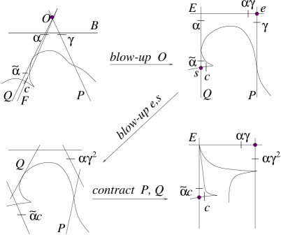
Figure 8:

To find a meridian of $Q_{n}$, first define a meridian $\tilde{\alpha}$ of $Q$ as shown in figure (8). That is, take a small disc $\Delta$ intersecting $Q$ transversally above the point $s$, and take a path $\omega$ joining $\Delta$ to a neighborhood $f_{3}$, and continuing to $*$ in $F^{\prime}$ along the loop $c$. Let $\tilde{\alpha}:=\omega\cdot\delta\cdot\omega^{-1}$. Then the blowing up of the point $s$ will give $\tilde{\alpha}c$ as a meridian of $Q_{1}$. A recursive application of Fujita’s Lemma gives $\mu(Q_{n}):=\tilde{\alpha}c^{n}$ as a meridian of $Q_{n}$.

Note that the construction of $C_{n}$ also shows that $\mu_{q}:=\alpha\gamma$ is a singular meridian of $C_{n}$ at $q_{n}$, since $\mu_{q}$ is a meridian of the exceptional line of the blow-up of $q_{n}$.

3.1.4 Finding $\tilde{\alpha}$

The final step in determining the fundamental group of $C_{n}$ is to express $\tilde{\alpha}$ in terms of the above presentation of $\pi_{1}(\mathbb{P}^{2}\backslash(C\cup P\cup Q))$. Let us show that $\tilde{\alpha}$ is in fact homotopic to $\alpha$.

First, let $\widetilde{\Delta}:=pr^{-1}(\Delta)\cap B$. Then $\alpha$ is clearly homotopic to a loop obtained by connecting (properly) $\partial\widetilde{\Delta}$ to the base point $*$. $\partial\widetilde{\Delta}$ intersect the real axis of $B$ at two points, let $*^{\prime}$ be the one on the right, which will be used as a temporary base point. Now push the fiber $F$ over $*^{\prime}$ along the real axis of $B$. As all the intersection points remains real, it is easy to see that the picture of $F$ stays as in Figure (3).

Next, consider the restriction $pr^{\prime}:{pr^{-1}(\partial\widetilde{\Delta})}\rightarrow\partial\widetilde{\Delta}$ of $pr$ to the border of the disc $\widetilde{\Delta}$. This is a locally trivial fibration, and it can be pictured as in Figure (9), where we have cut $\partial\widetilde{\Delta}$ at $*^{\prime}$ to give a better picture. Let $\Sigma$ be a disc in $F$, containing the upper intersection points $f_{1}$ and $f_{2}$ of $C$ with $F$, we suppose that $\Sigma$ avoids the loop $c$. Then, as the lower intersection point $f_{3}$ is a transversal intersection, we can suppose that the corresponding Leftschez homeomorphisms $F\rightarrow F_{t}$, $t\in\partial\widetilde{\Delta}$ are constant outside $\Sigma$. Hence, the following map gives a homotopy between $\alpha$ and $\tilde{\alpha}$.

Figure 9:

$$H(s,t):=\left\{\begin{array}[]{rl}(\alpha(0),\omega(t)),&0\leq t\leq s/3\\ (\alpha\left(\frac{t-s/3}{1-2s/3}\right),\omega(s/3)),&s/3\leq t\leq 1-s/3\\ (\alpha(1),\omega(1-t))&1-s/3\leq t\leq 1\end{array}\right.$$

Consequently, the vanishing of the meridian of $Q_{n}$ yields the relation

$$\mu(Q_{n})=1\Rightarrow\alpha=c^{-n}\quad({\cal R}_{8}).$$

Substituting $\alpha$ from $({\cal R}_{8})$, $({\cal R}_{7})$ becomes

$$c^{n^{2}}(cbc^{-n}b)^{n+1}=1.$$

From the cusp relation $cbc=bcb$ it follows that $cbc^{k}=b^{k}cb$ for any $k\in\mathbb{Z}$. Using this in the above relation, we get

$$c^{n^{2}}(b^{-n}cb^{2})^{n+1}=1\quad({\cal R}_{9}).$$

To sum up, we have the presentation

$$=\pi_{1}(\mathbb{P}^{2}\backslash C_{n})=\langle b,c,\alpha\,|\,{\cal R}_{3},\,{\cal R}_{4},\,{\cal R}_{5},\,{\cal R}_{7},\,{\cal R}_{9}\rangle.$$

3.1.5 Study of the group

Since $\alpha=c^{-n}$ by $({\cal R}_{7})$, the relation $({\cal R}_{3})$ is trivialized, and using the cusp relation $({\cal R}_{4})$ becomes

$$(bc^{-n})^{2}=(c^{-n}b)^{2}\Leftrightarrow[b^{n},c^{n+2}]=1.$$

Finally, we have obtained the presentation given in Theorem 2.4.

$$G_{n}:=\pi_{1}(\mathbb{P}^{2}\backslash C_{n})=\langle b,c\,|\,cbc=bcb,\quad[b^{n},c^{n+2}]=1,\quad(b^{-n}cb^{2})^{n+1}c^{n^{2}}=1\rangle.$$

Notice that $(c)$ is the unique class of meridian in $G_{n}$. Also, the singular meridian $\mu_{r}=cb$ of $C$ is unchanged during the birational transformations, so that $\mu_{r}$ is a singular meridian of $C_{n}$ at $r_{n}$. Other singular meridians are, as found above, $\mu_{q}=\alpha\gamma$ and $\mu_{p}=(\alpha\gamma)^{-1}$. One has $(\alpha\gamma)^{-1}=cba=cb\alpha b\alpha^{-1}=cbc^{-n}bc^{n}$.
It is easily seen that $G_{0}=\mathbb{Z}/3\mathbb{Z}$. Let us now show that $G_{1}=\mathbb{Z}/5\mathbb{Z}$ and $G_{2}=\mathbb{Z}/7\mathbb{Z}$. One has

$$G_{1}=\langle c,b,\,|\,cbc=bcb,\,[b,c^{3}]=1,\,(b^{-1}cb^{2})^{2}c=1\rangle.$$

Expanding the last relation, we get

$$b^{-1}c\cdot bcb^{2}\cdot c=b^{-1}c\cdot c^{2}bc\cdot c=b^{-1}c^{3}bc^{2}=c^{5}.$$

Thus,

$$[b,c^{3}]=1\Rightarrow[b,c^{6}]=[b,c^{-1}]=[b,c]=1\Rightarrow b=c.$$

Hence, $G_{1}$ is generated by $b$, and $G_{1}=\mathbb{Z}/5\mathbb{Z}$. The group $G_{2}$ has the presentation

$$G_{2}=\langle c,b\,|\,cbc=bcb,\quad[b^{2},c^{4}]=1,\quad(b^{-2}cb^{2})^{3}c^{4}=1\rangle.$$

Again, expanding the last relation we get

$$b^{-2}c^{3}b^{2}c^{4}=1\Rightarrow c^{7}=1.$$

Thus,

$$[b^{2},c^{4}]=1\Rightarrow[b^{6},c^{8}]=[b^{-1},c]=[b,c]=1\Rightarrow c=b.$$

Hence, $G_{2}$ is generated by $b$, and one has $G_{2}=\mathbb{Z}/7\mathbb{Z}$. The group $G_{3}$ is found to be finite of order $8640$ by using the programme Maple. The order of the group $G_{5}$ is calculated to be $1560$ by Artal by the help of the programme GAP.

Definition 3.2.

(residual group) For an element $a\in G$ of an arbitrary group $G$, the group $G/\ll a\gg$ will be denoted by $G(a)$. If $G_{C}:=\pi_{1}(\mathbb{P}^{2}\backslash C)$ is the group of an irreducible curve $C$, with $\mu$ a meridian of $C$, then for $k\in\mathbb{N}$, we will call the group $G_{C}(\mu^{k})$ a residual group of $G_{C}$ and denote it by $G_{C}(k)$. The group $G_{C}(\mu_{p}^{k})$, where $\mu_{p}$ is a singular meridian of $C$ at a singular point $p\in C$, will be called a residual group of $G_{C}$ at $p$ and denoted by $G_{C}^{p}(k)$. Note that the groups $G_{C}(k)$ do not depend on the particular meridian $\mu$ chosen, since by Lemma 1(ii), for an irreducible curve, any two meridians are conjugate. In view of Lemma 1(iii), this is also true for the groups $G_{C}^{p}(k)$.

Proposition 3.1.

If $n$ is odd, and $k|n$, then there is a surjection

$$G_{n}(k)\twoheadrightarrow T_{2,3,k}=\langle x,y,z\,|\,x^{2}=y^{3}=z^{k}=xyz=1\rangle$$

onto the triangle group $T_{2,3,k}$. Hence, $G_{n}$ is big for odd $n\geq 7$.

Proof.

For the last assertion, it is known that the group $T_{2,3,k}$ is big if $k\geq 7$. Putting $n=k$, we get that the groups $G_{n}(n)$ are big for $n\geq 7$ odd, so that $G_{n}$ is big if $n\geq 7$ is odd.

Now let us establish the surjection claimed. If $b^{k}=1$, then $c^{n}=b^{n}$=1 since $k|n$. This gives the presentation

$$G_{n}(k)=\langle b,c\,|\,cbc=bcb,\quad(cb^{2})^{n+1}=1,\quad b^{k}=1\rangle.$$

Following an idea due to Artal [1], we apply the transformation $x=cbc$, $y=cb$ ($\Leftrightarrow$ $c=y^{-1}x$, $b=x^{-1}y^{2}$) to obtain

$$G_{n}(k)=\langle x,y\,|\,x^{2}=y^{3},\quad(yx^{-1}y^{2})^{n+1}=1,\quad(y^{-1}x)^{k}=1\rangle.$$

Note that $yx^{-1}y^{2}=yxy^{-1}$ since $x^{2}=y^{3}$. Thus,

$$G_{n}(k)=\langle x,y\,|\,x^{2}=y^{3},\quad x^{n+1}=1,\quad(y^{-1}x)^{k}=1\rangle.$$

Let $H$ be the quotient of this group by the relation $x^{2}=y^{3}=1$ (note that $x^{2}$ is central). Then the relation $x^{n+1}=1$ is killed if $n$ is odd, and we get the desired result:

$$H=\langle x,y\,|\,x^{2}=y^{3}=(y^{-1}x)^{k}=1\rangle=T_{2,3,k}.\qquad\Box$$

This completes the proof of Theorem 2.4.

3.2 Groups of the curves (1)-(1a) in Theorem 2.9

3.2.1 Construction of the curves

Before passing to the construction of the curves, let us fix some notations following [4].

Notation. Let $\sigma_{O}:X_{1}\rightarrow\mathbb{P}^{2}$ be the blow-up of $\mathbb{P}^{2}$ at the point $O\in\mathbb{P}^{2}$. Denote by $E_{1}$ the exceptional divisor of this blow-up. For any curve $C\subset\mathbb{P}^{2}$, the proper preimage of $C$ in the Hirzebruch surface $X_{1}$ will be denoted by $C_{1}$. Now let $X_{i}$ be a Hirzebruch surface. Then $X_{i}$ is a ruled surface, whose horizontal section is denoted by $E_{i}$. Let $p\in X_{i}$, and let $L_{i}$ be the fiber of the ruling passing through $p$. The surface obtained from $X_{i}$ by an elementary transformation at the point $p$ will be denoted by $X_{i+1}$. Recall that this is a birational mapping which consists of blowing-up $p\in X_{i}$ followed by the contraction of $L_{i}$. The fiber replacing $L_{i}$ will be denoted by $L_{i+1}$, and for any curve $C_{i}\in X_{i}$, the proper transform of $C_{i}$ in $X_{i+1}$ will be denoted by $C_{i+1}$.

Let $n,m\in\mathbb{N}$ be such that $0\leq m<n$, and for $k\geq 2$, let $C$ be the curve defined by the equation $F(x,y,z):=xy^{k-1}-z^{k}=0$. Then for $k>2$, the curve $C$ has a unique singularity at $p:=[1:0:0]$ which is a cusp and $q=[0:1:0]$ is an inflection point of $C$ of order $k$. If $k=2$, then $p$ is a smooth point of $C$. The line $P:=\{y=0\}$ is the tangent to $C$ at $p$ and $Q:=\{x=0\}$ is the tangent at $q$, these tangents intersects at the point $O:=P\cap Q=[0:0:1]\notin C$. Blowing-up the point $O$, we get a Hirzebruch surface $X_{1}$. Let $E_{1}$ be its horizontal section, and denote by $P_{1}$, $Q_{1}$ the proper transforms of $P$ and $Q$ respectively. For $i=1,2,\dots,m$ we apply $m$ elementary transformations at the points $E_{i}\cap P_{i}$, followed by elementary transformations applied at the points $E_{i}\cap Q_{i}$ for $i=m+1,m+2,\dots,n$, and we arrive at the Hirzebruch surface $X_{n+1}$ with $E_{n+1}^{2}=-n-1$ (see Figure (12)).

Performing elementary transformations at arbitrary points $s_{i}\in P_{i}\backslash E_{i}$ for $i=n+1,\dots,2n$ we obtain the Hirzebruch surface $X_{2n+1}$ with $E_{2n+1}^{2}=-1$. Hence, one can contract $E_{2n+1}$ and return to the projective plane $\mathbb{P}^{2}$. Let $\widetilde{C},\widetilde{P},\widetilde{Q}$ be the images of respectively $C_{2n+1},P_{2n+1},Q_{2n+1}$ under the contraction of $E_{2n+1}$. Then $\widetilde{C}$ is a curve of the family (1).

The curves (1a) are obtained in the same way, except that in this case one applies elementary transformations at the points $E_{i}\cap P_{i}$ for $i=1,2,\dots,n$ followed by elementary transformations at some points $s_{i}\in E_{i}\cap Q_{i}$ for $i=n+1,n+2,\dots,2n$.

These birational morphisms provides a biholomorphism

$$\mathbb{P}^{2}\backslash(C\cup P\cup Q)\stackrel{{\scriptstyle\simeq}}{{\longrightarrow}}\mathbb{P}^{2}\backslash(\widetilde{C}\cup\widetilde{P}\cup\widetilde{Q}).$$

One has the induced isomorphism

$$\pi_{1}(\mathbb{P}^{2}\backslash(C\cup P\cup Q))\simeq\pi_{1}(\mathbb{P}^{2}\backslash(\widetilde{C}\cup\widetilde{P}\cup\widetilde{Q})).$$

3.2.2 Finding $\pi_{1}(\mathbb{P}^{2}\backslash(C\cup P\cup Q))$

We will apply the Zariski-Van Kampen method to the projection $pr:=\mathbb{P}^{2}\backslash{O}\rightarrow\mathbb{P}^{1}$. Clearly, $P$, $Q$ are singular fibers of this projection, and it is easy to see that these are the only ones. Indeed, a line passing through $O=[0:0:1]$ has an equation of the form $ax+by=0$. Comparing with the equation $xy^{k-1}-z^{k}=0$ of $C$, one obtains $by^{k}+az^{k}=0$, which has multiple solutions if and only if $a=0,b\neq 0$ or $a\neq 0,b=0$, corresponding to the lines $P=\{y=0\}$ and $Q=\{x=0\}$. Let $pr^{\prime}$ be the restriction of the projection $pr$ to $\mathbb{P}^{2}\backslash(C\cup P\cup Q)$.

Figure 10:

Let $L_{\infty}:=\{z=0\}$, and shift to the affine coordinates in $\mathbb{P}^{2}\backslash L_{\infty}=\mathbb{C}^{2}$. Let $B$ be the line $\{x+y=\epsilon\}$, where $\epsilon$ is a small real number and let $F:=\{x=y\}$ be the base fiber (Figure (10)-I). Put $B^{\prime}:=B\backslash(P\cup Q)$ and $F^{\prime}:=F\backslash(\{O\}\cup C)$. If we choose $L_{\infty}:=\{y=0\}$ and pass to the affine coordinates in $\mathbb{P}^{2}\backslash L_{\infty}=\mathbb{C}^{2}$, then the real picture of the configuration $C\cup P\cup Q$ will be as it is drawn in Figure (10)-II. Let $*:=F\cap B$ be the base point. Identify the fibers with $\mathbb{C}$ via the projection to the $z$-axis, and take the generators of $\pi_{1}(B^{\prime})$ and $\pi_{1}(F^{\prime})$ as in Figure (11).

Figure 11:

The monodromy relations around the singular fiber $Q$ are given by

$$\beta^{-1}a_{i}\beta=\left\{\begin{array}[]{ll}a_{i+1},&1\leq i\leq k-1,\\ \delta\;a_{1}\;\delta^{-1},&i=k.\end{array}\right.$$

where $\delta:=a_{k}a_{k-1}...a_{2}a_{1}$. Setting $a:=a_{1}$, these relations can be expressed as

$$a_{i}=\beta^{-i+1}a\beta^{i-1},\quad(\beta a)^{k}=(a\beta)^{k}.$$

Hence, one has the presentation

$$\pi_{1}(\mathbb{P}^{2}\backslash(C\cup T\cup L))=\langle\beta,a\quad|\quad(a\beta)^{k}=(\beta a)^{k}\rangle.$$

Note that $[\alpha,\beta]=1$ and $\alpha\beta a_{k}\cdots a_{2}a_{1}=1$. The change of generators $(\beta,\quad a)\Leftrightarrow(\beta,\quad y:=\beta a)$ gives a more convenient presentation

$$\pi_{1}(\mathbb{P}^{2}\backslash(C\cup T\cup L))=\langle\beta,y\;|\;[\beta,y^{n}]=1\rangle.$$

For the future applications, note that $\alpha$ can be expressed by using the relation

$$\alpha\beta a_{k}a_{k-1}\cdots a_{1}=1\Leftrightarrow\alpha=y^{-k}\beta^{k-1}.$$

Note also that $[\alpha,\beta]=1$. This can be derived either from the above presentation or by applying Fujita’s lemma to the meridians $\alpha$ of $P$ and $\beta$ of $Q$, with respect to the point $O=P\cup Q$.

3.2.3 Meridians of $\widetilde{P}$ and $\widetilde{Q}$

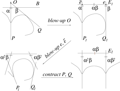
Figure 12:

An obvious application of Fujita’s lemma yields that $\mu(P_{n+1}):=\alpha(\alpha\beta)^{m}$ is a meridian of $P_{n+1}$ and $\mu(Q_{n+1}):=\beta(\alpha\beta)^{n-m}$ is a meridian of $Q_{n+1}$ in the surface $X_{n+1}\backslash(C_{n+1}\cup P_{n+1}\cup Q_{n+1}\cup E_{n+1})$. (See Figure (12), where the situation is illustrated for $n=2$, $m=1$, beware that the elementary transformation applied at $e:=E_{1}\cap P_{1}$ and the elementary transformation applied at $\tilde{e}:=E_{2}\cap Q_{2}$ are shown simultaneously in the figure.) Recall that the subsequent transformations are applied at points $s_{i}\in E_{i}\backslash P_{i}$ for $i=n+1,\dots,2n$. Since the line $Q_{n+1}$ is not affected by these transformations, $\mu(Q_{n+1})$ is a meridian of $\widetilde{Q}$ in $\mathbb{P}^{2}\backslash(\widetilde{C}\cup\widetilde{P}\cup\widetilde{Q})$, too.

On the other hand, $\mu(P_{n+1})$ stays to be a meridian of $P_{n+i}$ after an elementary transformation applied at a point $s_{i}\in E_{i}\backslash P_{i}$. This can be seen e.g. by choosing $s_{n+1}=\Delta\cap P_{n+1}$, where $\Delta$ is the defining disc of $\mu(P_{n+1})$. Hence, $\mu(P_{n+1})$ is a meridian of $\widetilde{P}$, too.

Denote by $\tilde{p}$ and $\tilde{q}$ the cusps of $\widetilde{C}$. Then, by the construction of the curve, $\alpha\beta$ is a singular meridian at $\tilde{p}$, and $\beta(\alpha\beta)^{n-m-1}$ is a singular meridian at $\tilde{q}$.

Setting $\mu(P_{n+1})=\mu(Q_{n+1})=1$, we obtain the presentation

$$G_{(1)}:=\pi_{1}(\mathbb{P}^{2}\backslash\widetilde{C})=$$

$$\langle\alpha,\beta,y\,|\,\alpha=y^{-k}\beta^{k-1},\quad[\beta,y^{k}]=\alpha(\alpha\beta)^{m}=\beta(\alpha\beta)^{n-m}=1\rangle.$$

A meridian of $\widetilde{C}$ can be given as $a=\beta^{-1}y$. After the obvious simplifications, one finds that $\alpha\beta=y^{-k}\beta^{k}$ is a singular meridian at $\tilde{p}$, and $(\alpha\beta)^{-1}=y^{k}\beta^{-k}$ is a singular meridian at $\tilde{q}$.

It is easy to see that the element $y^{k}$ is central in the group $G_{(1)}$. Eliminating $\alpha$ in $G_{(1)}(y^{k})$, one obtains

$$G_{(1)}(y^{k})=\langle\beta,y\,|\,y^{k}=\beta^{j}=1\rangle=\mathbb{Z}_{k}*\mathbb{Z}_{j},$$

where $j:=\mbox{g.c.d.}(mk+k-1,nk-mk+1)=\mbox{g.c.d.}(mk+k-1,kn+k)=\mbox{g.c.d.}(mk+k-1,n+1)$. Hence, this group is big if $j\geq 2$. Finally, the group $G_{(1)}$ is abelian when $j=1$ by the following trivial lemma:

Lemma 3.

Let $G$ be a group, and $z\in G$ be a central element. If $G(z)$ is cyclic, then $G$ is abelian.

As for the curves from the family (1a), the same procedure applies. The meridian $\beta$ of $Q$ stays to be a meridian of $\widetilde{Q}$, so that one has the relation $\beta=1$, which implies that the fundamental group is generated by just one element $y(=a)$ and thus it is abelian.

Remark. In [3], the authors provide a long argument due to V. Lin, showing the bigness of the group given by the presentation $\langle a,b\,|\,(ab)^{2}=(ba)^{2}\rangle$. Here is a simpler proof of a more general assertion:

Proposition 3.2.

Let $n,m\in\mathbb{Z}$ such that $k:=gcd\,(n,m)$ satisfy $|k|\geq 2$. Then the group

$$\langle a,b\,|\,(ab)^{n}=(ba)^{m}\rangle$$

is big.

Proof.

Put, as above, $x:=ab$ and $y:=b$. Then the above presentation is written in terms of $x,y$ as

$$\langle x,y\,|\,x^{n}=yx^{m}y^{-1}\rangle.$$

Passing to the quotient by the relation $x^{k}=1$, we get the group $\mathbb{Z}_{k}*\mathbb{Z}$, which is big. This can be seen as follows: Let $r\geq 3$ be an integer such that $gcd\,(r,k)=1$. Passing once more to the quotient by the relation $y^{r}=1$ gives the group $\mathbb{Z}_{k}*\mathbb{Z}_{r}$, and it is well known that the commutator subgroup of this group is the free group of rank $(k-1)(r-1)$. $\Box$

Note that the group $\mathbb{Z}_{2}*\mathbb{Z}_{2}$ is isomorphic to the infinite dihedral group ${\mathbb{D}}_{\infty}$, whose commutator subgroup is $\mathbb{Z}$, hence this group is solvable and is not big. Also, it can be shown that the commutator subgroup of the group $\langle a,b\,|ab=(ba)^{2}\rangle$ is abelian, but not finitely generated.

3.2.4 Groups of the curves (2)-(2a)

These curves are constructed as the curves (1)-(1a) with the following difference: One performs elementary transformations at the points $E_{i}\cap Q_{i}$ for $i=1,2,\dots,m$ followed by elementary transformations at the points $E_{i}\cap P_{i}$ for $i=m+1,m+2,\dots,n$. Finally, for $i=n,n+1\dots,2n$ one applies elementary transformations at some points $s_{i}\in Q_{i}\backslash E_{i}$. The curves (2a) are obtained by setting $n=m$ in the above procedure.

The same reasoning as in the case of the curves (1)-(1a) shows that $\mu(Q_{m+1}):=\beta(\alpha\beta)^{m}$ is a meridian of $\widetilde{Q}$, and $\mu(P_{m+1}):=\alpha(\alpha\beta)^{m-n}$ is a meridian of $\widetilde{P}$. Setting $\mu(Q_{m+1})=\mu(P_{m+1})=1$, we obtain the presentation

$$G_{(2)}:=\pi_{1}(\mathbb{P}^{2}\backslash\widetilde{C})=$$

$$\langle\alpha,\beta,y\,|\,\alpha=y^{-k}\beta^{k-1},\quad[\beta,y^{k}]=\beta(\alpha\beta)^{m}=\alpha(\alpha\beta)^{n-m}=1\rangle.$$

Obviously, $\alpha\beta$ and $(\alpha\beta)^{-1}$ are singular meridians at $\tilde{q}$ and $\tilde{p}$, respectively. A meridian of $\widetilde{C}$ can be given as $a=\beta^{-1}y$.

For the curves (2a) we obtain,

$$G_{(2a)}:=\pi_{1}(\mathbb{P}^{2}\backslash\widetilde{C})=$$

$$\langle\alpha,\beta,y\,|\,\alpha=y^{-k}\beta^{k-1},\quad[\beta,y^{k}]=\alpha^{m}\beta^{m+1}=\alpha=1\rangle.$$

$$=\langle\beta,y\,|\,y^{-k}=\beta^{k-1},\quad\beta^{n+1}=1\rangle.$$

Meridians in this case can be obtained from those of the case (2) by putting $\alpha=1$.

Again, the element $y^{k}$ is central in the group $G_{2}$, and one has

$$G_{(2)}(y^{k})=\langle y,\beta\,|\,y^{k}=1,\quad\beta^{j}=1\rangle=\mathbb{Z}_{k}*\mathbb{Z}_{j},$$

where this time $j:=\mbox{g.c.d.}(1+mk,nk-mk+k-1)=\mbox{g.c.d.}(1+mk,nk+k)=\mbox{g.c.d.}(1+mk,n+1)$.

As for the curves (2a) we obtain,

$$G_{(2a)}(y^{k})=\langle y,\beta\,|\,y^{k}=1,\quad\beta^{j}=1\rangle=\mathbb{Z}_{k}*\mathbb{Z}_{j},$$

where $j=\mbox{g.c.d.}(k-1,n+1)$.

3.3 Groups of the curves (3)

Let $C$ be the curve defined by the equation $xy^{k}-z^{k+1}=0$, the point $p$ be its cusp, $q$ its inflection point, and $R$ be the line $\overline{pq}=\{z=0\}$. Let, as in the case (1), $P$, $Q$ be the tangent lines at $p$, $q$, respectively.
Blowing-up the inflection point $q=[0:1:0]$ we get the Hirzebruch surface $X_{1}$. For $i=1,2,\dots,n$, we perform elementary transformations at the points $E_{i}\cap R_{i}$, followed by elementary transformations at some points $s_{i}\in Q_{i}\backslash E_{i}$, and we end up with a Hirzebruch surface $X_{2n+1}$ with $E_{2n+1}^{2}=1$. Let $\widetilde{C}$, $\widetilde{R}$, $\widetilde{Q}$ be the images of $C_{2n+1}$ ,$R_{2n+1}$, $Q_{2n+1}$ in $\mathbb{P}^{2}$ under the contraction of $E_{2n+1}$. Then $\widetilde{C}$ is a curve from the family (3). One has the biholomorphic map

$$\mathbb{P}^{2}\backslash(C\cup R\cup Q)\stackrel{{\scriptstyle\simeq}}{{\longrightarrow}}\mathbb{P}^{2}\backslash(\widetilde{C}\cup\widetilde{R}\cup\widetilde{Q}),$$

inducing an isomorphism

$$\pi_{1}(\mathbb{P}^{2}\backslash(C\cup R\cup Q))\simeq\pi_{1}(\mathbb{P}^{2}\backslash(\widetilde{C}\cup\widetilde{R}\cup\widetilde{Q})).$$

In order to find $\pi_{1}(\mathbb{P}^{2}\backslash(C\cup R\cup Q))$, we shall use the projection from the point $O:=P\cap Q$, as before. As the only points of intersection $R\cap C$ are $p$ and $q$, this projection has only two singular fibers, namely $P$ and $Q$. Choose the base $B$ and the generic fiber $F$ as in Figure (10).

Figure 13:

Let $F^{\prime}:=F\backslash(C\cup\{O\}\cup R)$, and choose the generators $a_{1},\dots a_{k+1},\gamma$ for $\pi_{1}(F^{\prime})$ as in Figure (13). The monodromy relations around $Q$ are given by

$\beta^{-1}a_{i}\beta=\left\{\begin{array}[]{ll}a_{i+1},&1\leq i\leq k,\\ (\delta\gamma)\;a_{1}\;(\delta\gamma)^{-1},&i=k+1,\end{array}\right.$

$\beta^{-1}\gamma\beta=$ $\qquad a_{1}\gamma a_{1}^{-1}.\qquad\qquad$

where $\delta:=a_{k+1}a_{k}...a_{2}a_{1}$. Observe that, as $\beta$ is a meridian of $Q$, and as the elementary transformations are applied at points $s_{i}\in Q_{i}\backslash E_{i}$, $\beta$ is a meridian of $Q_{i}$, and thus it is a meridian of $\widetilde{Q}$. Imposing the relation $\beta=1$ in the relations found above, we find that $a_{1}=a_{2}=\dots=a_{k+1}$, and $[a_{1},\gamma]=1$. Since the group $\pi_{1}(\mathbb{P}^{2}\backslash\widetilde{C})$ is generated by these elements we conclude that it is abelian.

3.4 Groups of the curves (4)

We begin by the curve $C:=xy^{k}-z^{k+1}$. Let $Q:=\{x=0\}$ be the tangent to $C$ at its flex $q:=[0:1:0]$, and let $P$ be a line intersecting $C$ transversally at its cusp $p:=[1:0:0]$, and such that $q\notin P$. Then by Bezout’s theorem, $P$ intersects $C$ at one further point $r\neq q$. Let $O:=P\cap Q$. Blowing-up $O$, we get the Hirzebruch surface $X_{1}$, with the horizontal section $E_{1}$ with $E_{1}^{2}=-1$. For $i=1,2,\dots,n$, apply elementary transformations at the points $r_{i}$ followed by elementary transformations applied at the points $E_{i}\cap Q_{i}$. Then $E_{2n+1}^{2}=-1$; contracting it, we turn back to the projective plane $\mathbb{P}^{2}$. Let $\widetilde{C}$, $\widetilde{P}$, $\widetilde{Q}$ be the images of $C_{2n+1}$, $P_{2n+1}$ $Q_{2n+1}$ under this contraction. Then $\widetilde{C}$ is a curve of the family (4), and one has the biholomorphism

$$\mathbb{P}^{2}\backslash(C\cup P\cup Q)\stackrel{{\scriptstyle\simeq}}{{\longrightarrow}}\mathbb{P}^{2}\backslash(\widetilde{C}\cup\widetilde{P}\cup\widetilde{Q}),$$

inducing an isomorphism of the fundamental groups.
To find the group of $C\cup P\cup Q$, we shall use the projection from the point $O$. In addition to $P$ and $Q$, this projection has a third singular fiber $R$, which is a simple tangent to $C$ at a unique, smooth point of $C$. That $P$, $Q$, $R$ are the only singular fibers can be seen by looking at the dual picture. Indeed, by the class formula, one has

$$d^{*}=2(g-1+k+1)-(k-1)=k+1$$

where $g=0$ is the genus of $C$, and $d^{*}$ is the degree of the dual curve $C^{*}$. Now, the point $Q^{*}\in{\mathbb{P}^{2}}^{*}$ is a cusp of $C^{*}$ with multiplicity $k$. Hence, the line $O^{*}$ which passes through $Q^{*}$ should intersect $C^{*}$ transversally at a unique further point $R^{*}$, which is the dual of the simple tangent line $R$ from $O$ to $C$.

Now we apply the change of coordinates

$$[x:y:z]\Rightarrow[x+y:y:z].$$

In the new coordinates, the equation of $C$ reads as $(x-y)y^{k}-z^{k+1}=0$. Let $L_{\infty}$ be the line $x=0$, and pass to the affine coordinates $(y/x,z/x)$ in $\mathbb{C}^{2}=\mathbb{P}^{2}\backslash L_{\infty}$. Recall that we have the freedom to choose $O$ (or, equivalently, $P$). So let $O=(1,z_{0})$, where $z_{0}$ is a big real number.

Figure 14:

The real picture of the configuration $C\cup P\cup Q\cup R$ is shown in Figure (14). Choose the base fiber $F$, and the base of the projection as in Figure (14). Put $F^{\prime}:=F\backslash(C\cup O)$ and $B^{\prime}:=B\backslash(P\cup Q\cup R)$. Take the generators $b,a_{1},a_{2},\dots,a_{k}$ for $\pi_{1}(F^{\prime})$ as in Figure (15)-I and the generators $\alpha$, $\beta$, $\gamma$ for $\pi_{1}(B^{\prime})$ as in Figure (15)-III.

Figure 15:

The monodromy around $R$ yields (after setting $\gamma=1$),

$$a_{1}=b\quad({\cal R}_{1}),$$

and the monodromy around $P$ gives

$\beta^{-1}a_{i}\beta=\left\{\begin{array}[]{rl}\delta a_{i+1}\delta^{-1}&1\leq i<k,\\ \delta^{2}a_{1}\delta^{-2}&i=k,\end{array}\right.\quad({\cal R}_{2})$,

where $\delta:=a_{k}a_{k-1}\cdots a_{1}$. Hence, we have the presentation

$$\pi_{1}(\mathbb{P}^{2}\backslash(C\cup P\cup Q\cup R))=\langle\beta,b,a_{1},a_{2},\dots,a_{k}\,|\,({\cal R}_{1}),\,({\cal R}_{2})\rangle$$

Note that $\alpha\beta\delta b=1$, and that $[\alpha,\beta]=1$.

An obvious application of Fujita’s Lemma shows that $\beta b^{n}$ is a meridian of $\widetilde{P}$ and $\alpha(\alpha\beta)^{n}$ is a meridian of $\widetilde{Q}$. Therefore,

$$G_{(4)}:=\pi_{1}(\mathbb{P}^{2}\backslash\widetilde{C})=\langle\beta,b,a_{1},a_{2},\dots,a_{k}\,|\,\beta b^{n}=\alpha(\alpha\beta)^{n}=1,\,({\cal R}_{1}),\,({\cal R}_{2})\rangle.$$

3.4.1 Study of the group

By using $({\cal R}_{2})$, one can express the generators $a_{1},a_{2},\dots,a_{k}$ in terms of $b$ as follows

$$a_{i}=(\beta\delta)^{-i+1}b(\beta\delta)^{i-1}\qquad 1\leq i\leq k.$$

Then, the last relation in $({\cal R}_{2})$ reads

$$(\beta\delta)^{-k}b(\beta\delta)^{k}=\delta b\delta^{-1}\quad({\cal R}_{3}).$$

For $\delta$, one has

$$\delta=a_{k}a_{k-1}\cdots a_{1}=(\beta\delta)^{-k}(\beta\delta b)^{k}\quad({\cal R}_{4}).$$

Since $\alpha=(\beta\delta b)^{-k}$, the relation $\alpha^{n+1}\beta^{n}=1$ becomes

$$(\beta\delta b)^{n+1}b^{n^{2}}=1\quad({\cal R}_{5}),$$

where we have used $\beta=b^{-n}$. This gives the presentation

$$G_{(4)}=\langle\beta,\delta,b\,|\,\delta=(\beta\delta)^{-k}(\beta\delta b)^{k},\quad\beta=b^{-n},\quad(\beta\delta b)^{n+1}b^{n^{2}}=1,\quad(\beta\delta)^{-k}b(\beta\delta)^{k}=\delta b\delta^{-1}\rangle.$$

Now put $x:=\beta\delta$ and $y:=b$. Then $\delta=\beta^{-1}x=y^{n}x$, and one can rewrite the above presentation as

$$G_{(4)}=\langle x,y\,|\,(xy)^{n+1}y^{n^{2}}=[y,x^{k}y^{n}x]=1,\quad x^{k}y^{n}x=(xy)^{k}\rangle,$$

since $({\cal R}_{3})$ becomes

$$x^{-k}yx^{k}=y^{n}xyx^{-1}y^{-n}\,\Leftrightarrow\,[y,x^{k}y^{n}x]=1,$$

and for $({\cal R}_{4})$ one has

$$y^{n}x=x^{-k}(xy)^{k}\,\Leftrightarrow\,x^{k}y^{n}x=(xy)^{k}.$$

Finally, $({\cal R}_{5})$ is written as $(xy)^{n+1}y^{n^{2}}=1$. Note that $y=b$ is a meridian of $\widetilde{C}$.

Obviously, the latter presentation is equivalent to the presentation

$$G_{(4)}=\langle x,y\,|\,(xy)^{n+1}y^{n^{2}}=[y,(xy)^{k}]=1,\quad x^{k}y^{n}x=(xy)^{k}\rangle\qquad(*)$$

To simplify this presentation further, put $z:=xy$. Then $x=zy^{-1}$, and one obtains the presentation

$$G_{(4)}=\langle z,y\,|\,z^{n+1}y^{n^{2}}=[y,z^{k}]=1,\quad(zy^{-1})^{k}y^{n}zy^{-1}=z^{k}\rangle$$

It is readily seen from this presentation that the element $z^{k}$ is central. Passing to the quotient by $z^{k}$ gives

$$G_{(4)}(z^{k})=\langle z,y\,|\,z^{n+1}y^{n^{2}}=1,\quad(zy^{-1})^{k+1}y^{n}=z^{k}=1\rangle.$$

Now put $j:=gcd(n+1,k)$. Then one has

$$G_{(4)}(z^{k})(y^{n})=\langle z,y\,|z^{j}=y^{n}=(zy^{-1})^{k+1}=1\rangle=T_{j,n,k+1},$$

so that this latter group is big if

$$\frac{1}{j}+\frac{1}{n}+\frac{1}{k+1}<1.$$ (1)

Obviously, $G_{(4)}(z^{k})$, and hence also $G_{(4)}$ is abelian if $j=1$ or $n=1$. So suppose that $n,j\geq 2$.

First we consider the case $k=2$. Since $j\geq 2$, this forces $n\geq 3$ to be odd. If $n\geq 7$, then 1 is satisfied. In case $n=3$ or $n=5$, 1 is violated.

Now assume $k=3$. Then $j=3$ by the assumption $j\geq 2$, which forces $n+1\geq 3$ to be a multiple of $3$. For $n+1\geq 6$, 1 is not violated. For $n=2$, 1 is violated.

For $k\geq 4$, first assume that $k$ is even. Then the least value that $j$ can take is $2$, and the least value that $n$ can take is $3$. If $n=3$, then $j=4$, and 1 is not violated. But if $n\geq 4$, then 1 is not violated neither.

If $k\geq 4$ is odd, then the least divisor of $k$ is $3$, hence $j\geq 3$, and $k\geq 6$. In this case 1 is never violated.

This leaves the cases $(d,n,k)=(9,3,2)$, $(d,n,k)=(13,5,2)$, and $(n,k)=(10,2,3)$ open. Calculations with Maple show that these are finite groups of order 72, 1560 and 240 respectively.

Notice that when $k=2$, the degree of the curves (4) is $2n+3$, so it is interesting to compare their groups with the groups in Theorem 3.2.2. For $k=2$, the relation $x^{2}y^{n}x=(xy)^{k}$ in the presentation (*) above becomes

$$x^{2}y^{n}x=xyxy\quad\Leftrightarrow xy^{n}x=yxy\quad(**).$$

Now put

$$\alpha:=y,\quad\beta:=xy^{n-1}.$$

Then

$$y=\alpha,\quad x=\beta\alpha^{1-n},$$

and the relation (**) becomes the braid relation $\beta\alpha\beta=\alpha\beta\alpha$. On the other hand, the relation $[y,(xy)^{k}]=1$ in the presentation (*) is written, in terms of $\alpha$, $\beta$, as $[\alpha,\beta^{n}]=1$. Finally, the relation $(xy)^{n+1}y^{n^{2}}=1$ in (*) becomes

$$(\beta\alpha^{2-n})^{n+1}\alpha^{n^{2}}=1.$$

Hence, the presentation

$$\langle\alpha,\beta\,|\,\beta\alpha\beta=\alpha\beta\alpha,\quad[\alpha,\beta^{n}]=(\beta\alpha^{2-n})^{n+1}\alpha^{n^{2}}=1\rangle.$$

3.5 Groups of the curves (5)

Let $C$ be the curve $\{xy^{k-1}-z^{k}-z^{k-1}y\}$. Its unique singularity is a cusp at the point $p:=[1:0:0]$, and it has a flex of order $k-1$ at the point $q:=[0:1:0]$. Let $P$, $Q$ be the tangents to $C$ at $p$ and $q$. By Bezout’s theorem, $Q$ intersect $C$ at a third point $r$. Blowing-up the point $O:=P\cap Q$, we get the Hirzebruch surface $X_{1}$. Perform $n$ elementary transformations at $E_{i}\cap P_{i}$, followed by $n$ elementary transformations at the points $r_{i}$. One obtains the Hirzebruch surface $X_{2n+1}$ with $E_{2n+1}^{2}=-1$. Contraction of $E_{2n+1}$ gives the projective plane $\mathbb{P}^{2}$; denote by $\widetilde{C}$, $\widetilde{P}$, $\widetilde{Q}$ the images of $C$, $P$ and $Q$. Then $\widetilde{C}$ is a curve of the family (5).

To find $\pi_{1}(\mathbb{P}^{2}\backslash(C\cup P\cup Q))$, we shall use the projection from the point $O$. Evidently, $P$ and $Q$ are singular fibers of this projection. There is one further singular fiber say $R$, which is tangent to $C$ at a unique smooth point of $C$. Indeed, by the class formula, one has $d^{*}=k+1$. The point $Q^{*}\in{\mathbb{P}^{2}}^{*}$ is a cusp of multiplicity $k-1$. The line $O^{*}$ intersect $C^{*}$ at $P^{*}$, which is a smooth point of $C^{*}$, and at the cusp $Q^{*}$. By Bezout’s theorem, $O^{*}$ should intersect $C^{*}$ at a third point $R^{*}$ transversally, which is the point dual to the line $R^{*}$. This reasoning shows also that there are no other singular fibers.

In the affine coordinates $(x,z)$, the equation of $C$ reads $x=z^{k}+z^{k+1}$, and it is easy to see that the third singular fiber is the tangent line at $z=-k/(k+1)$.

Figure 16:

For $k$ even, the situation is pictured in Figure (16). Choose the base $B$ and the fiber $F$ as in the Figure (16), define $F^{\prime}$, $B^{\prime}$ as usual, and choose the generators for their fundamental groups as in Figure (17).

Set $\delta:=a_{k}a_{k-1}...a_{2}a_{1}$. Then the monodromy around $Q$ yields the relations

$$\beta^{-1}a_{i}\beta=\left\{\begin{array}[]{ll}a_{i+1},&1\leq i\leq k-1,\\ \delta\;a_{1}\;\delta^{-1},&i=k,\end{array}\right.\quad[\beta,b]=1$$

and the monodromy around $R$ gives

$$a_{k}=b$$

Figure 17:

Now, the relation $\beta^{-1}a_{k-1}\beta=a_{k}=b$ implies $a_{k-1}=b$, since $[\beta,a_{k}]=1$. Similarly, one obtains $a_{1}=a_{2}=\cdots=a_{k}=b$. This shows that $\pi_{1}(\mathbb{P}^{2}\backslash(C\cup P\cup Q))$ is abelian, which implies that $\pi_{1}(\mathbb{P}^{2}\backslash\widetilde{C})$ is abelian, too.

3.6 Groups of the curves (6) in Theorem 2.9

Let $C$ be the curve $\{xy^{k+1}-z^{k+2}-z^{k+1}y=0\}$, and let $Q$ be its tangent line at the inflection point $q$. Denote by $S$ the line $\overline{pq}$. The line $Q$ intersects $C$ at a second point $r$. Blowing-up the point $q$, we get the Hirzebruch surface $X_{1}$ with the horizontal section $E_{1}$. For $i=1,2,\dots,n$, perform elementary transformations at $E_{i}\cap S_{i}$, followed by elementary transformations at the points $r_{i}$ for $i=n+1,n+2,\dots,2n$. We end up with the Hirzebruch surface $X_{2n+1}$, with $E_{2n+1}=-1$. Contraction of $E_{2n+1}$ gives the projective plane $\mathbb{P}^{2}$, denote by $\widetilde{S}$, $\widetilde{Q}$, $\widetilde{C}$ the images of $S$, $Q$, and $C$ under this contraction.

The calculation of $\pi_{1}(\mathbb{P}^{2}\backslash(C\cup S\cup Q))$ will be realized by using the projection from the point $O:=P\cap Q$, where $P$ is the tangent to $C$ at its cusp as usual. The real picture is as in Figure (16), except that we should take the line $S=\overline{pq}=\{z=0\}$ into consideration. Now, the only points of intersection of the line $S$ with $C$ are the points $p$ and $q$. Hence, the only singular lines of the projection from the point $O$ are $P$, $Q$, and $R$, where $R$ is the simple tangent line from $O$ to $C$, as shown in the previous section.

Choose a fiber $F$ and a base $B$ as in Figure (16)-I, and put $F^{\prime}:=F\backslash(C\cup S\cup\{O\})$, $B^{\prime}:=B\backslash(P\cup Q\cup R)$. The situation is illustrated in Figure (18).

Figure 18:

Choose the generators $a_{1},a_{2},\dots,a_{k+1},b,\gamma$ for $\pi_{1}(F^{\prime})$, and the generators $\alpha,\beta$ for $\pi_{1}(B^{\prime})$ as in Figure (19).

Figure 19:

The monodromy around the singular fiber $Q$ gives

$$\beta^{-1}a_{i}\beta=\left\{\begin{array}[]{rl}a_{i+1},&1\leq i\leq k,\\ (\delta\gamma)a_{1}(\delta\gamma)^{-1},&i=k+1,\end{array}\right.\quad[\beta,b]=1,$$

where $\delta:=a_{k+1}a_{k}\cdots a_{1}$. From the monodromy around $R$ we get,

$$a_{k+1}=b.$$

These relations yields a presentation of the group $\pi_{1}(\mathbb{P}^{2}\backslash(C\cup S\cup Q))$.

Applying Fujita’s Lemma to the elementary transformations applied at the points $r_{i}$, we obtain the relation $\beta b^{n}=1$. Imposing this relation on the relations found above, we find that $a_{1}=a_{2}=\cdots=a_{k+1}=b$, and $[b,\gamma]=1$. We conclude that the group is abelian.

3.7 Groups of the curves (7) in Theorem 2.9

Let $C$ be the curve $xy^{k-1}-z^{k}=0$, with $p:=[1:0:0]$ as its cusp, $q:=[0:1:0]$ as its inflection point, and $P$, $Q$ as the tangents to $C$ at these points. Blow-up the point $O:=P\cap Q$, to get the Hirzebruch surface $X_{1}$, with the horizontal section $E_{1}$. Perform an elementary transformation at $q_{1}$, followed by an elementary transformation at $E_{2}\cap P_{2}$. Now for $i=3,4,\dots,n+2$ perform elementary transformations applied at the points $E_{i}\cap P_{i}$, followed by elementary transformations applied at some points $s_{i}\in Q_{i}\backslash E_{i}$ for $i=n+3,n+4,\dots,2n+2$. We end up with a Hirzebruch surface $X_{2n+3}$ with $E_{2n+3}=-1$. Contraction of $E_{2n+3}$ gives the projective plane $\mathbb{P}^{2}$.

We shall use the projection from the point $O$ to find the fundamental group. This projection has, in addition to $P$ and $Q$, a third singular fiber $R$, which is a simple tangent from $O$ to $C$ at a unique point. The setting is same as in Case 4, see Figure (14). Choose a base fiber close to $Q$, and take the generators for the base and the fiber as in Figure (15). The monodromy around $Q$ gives the relations

$$\beta^{-1}a_{i}\beta=\left\{\begin{array}[]{ll}a_{i+1},&1\leq i\leq k-1,\\ \delta a_{1}\delta^{-1},&i=k,\end{array}\right.$$

where $\delta:=a_{k}a_{k-1}\cdots a_{1}$.

Now, without finding the monodromy around $R$ or $P$, notice that an obvious application of Fujita’s lemma gives $a_{1}\beta$ as a meridian of $Q_{1}$. Subsequent elementary transformations on $Q_{i}$ are applied at some points $s_{i}\in Q_{i}\backslash E_{i}$, so that $a_{1}\beta$ stays to be a meridian of $Q_{i}$. Imposing the relation $a_{1}\beta=1$ on the above relations gives $\beta^{-1}=a_{1}=a_{2}=\cdots=a_{k}$. But, the group $\pi_{1}(\mathbb{P}^{2}\backslash(C\cup P\cup Q))$ is generated by the elements $a_{1},a_{2},\dots,a_{k},\beta$. Hence, the fundamental groups of the curves of the family (7) are abelian.

3.8 Groups of the curves (8) in Theorem 2.9

Let $C$ be the curve $xy^{2}-z^{3}=1$. Pick an arbitrary smooth point $q\in C$ which is not the inflection point of $C$, and let $Q$ be the tangent of $C$ at $q$. Put $P:=\overline{pq}$, where $p$ is the cusp of $C$.

By Bezout’s theorem, the line $Q$ intersect $C$ at a second point, say $r$.

Blowing-up the point $q$, we get the Hirzebruch surface $X_{1}$, with the horizontal section $E_{1}$. For $i=1,2,\dots,n-1$, perform elementary transformations at the points $r_{i}$, followed by elementary transformations performed at the points $E_{i}\cap P_{i}$ for $i=n,n+1,\dots,2n-2$. We end up with the Hirzebruch surface $X_{2n-2}$ with $E_{2n-1}^{2}=-1$. Contraction of $E_{2n+1}$ gives the projective plane $\mathbb{P}^{2}$ back. Denote as usual by $\widetilde{P}$, $\widetilde{Q}$, $\widetilde{C}$ the images of $P$, $Q$, $C$ under this contraction. Then $\widetilde{C}$ is a curve of the family (8).

Let us show that the group $\pi_{1}(\mathbb{P}^{2}\backslash(C\cup P\cup Q))$ is abelian, thereby showing that the groups of the curves of the family (8) are abelian.

Consider the singular projection from the cusp $p$. A generic fiber of this projection intersects $C\cup P\cup Q$ at two points, i.e. $\pi_{1}(\mathbb{P}^{2}\backslash(C\cup P\cup Q))$ is generated by two elements. These two points meet at the point $r$, which is a transversal intersection of $Q$ with $C$. This implies that the corresponding generators commute. It follows that $\pi_{1}(\mathbb{P}^{2}\backslash(C\cup P\cup Q))$ is abelian. $\Box$

3.9 Groups of the curves in Theorem 2.10

Let $C$ be the curve $(yz-x^{2})^{2}-x^{3}y=0$.

Lemma 4.

(Fenske [5]) $C$ is a rational cuspidal quartic with cusps at the point $p:=[0:0:1]$ of type $[2_{2}]$, and at the point $r:=[0:1:0]$ of type $[2_{1}]$. This curve has an inflection point of order $3$ at the point $q:=[-576:-4096:135]$.

Let $P$ be the tangent to $C$ at the cusp $p$, and let $Q$ be the inflectional tangent line at $q$. The cusp $p$ is the only intersection point of $P$ with $C$, whereas $Q$ intersect $C$ at a second further point, say $s$. It is clear that the point $O:=P\cup Q$ does not lie on $C$. Blowing-up $O$, we get the Hirzebruch surface $X_{1}$, with a section $E_{1}$ such that $E_{1}^{2}=-1$. Now for $i=1,2,\dots,n$ perform elementary transformations at the points $s_{i}$, followed by elementary transformations applied at the points $E_{i}\cup P_{i}$ for $i=n+1,n+2,\dots,2n+1$. We end up with the Hirzebruch surface $X_{2n+1}$ with $E_{2n+1}^{2}=-1$. Contraction of $E_{2n+1}^{2}=-1$ gives the projective plane $\mathbb{P}^{2}$. Denote by $\widetilde{C}$, $\widetilde{P}$, $\widetilde{Q}$ the images of $C_{2n+1}$, $P_{2n+1}$, $Q_{2n+1}$ under this contraction. Then $\widetilde{C}$ is the desired curve of degree $3n+4$.

To find the fundamental group of $C\cup P\cup Q$, we shall use the projection from the center $O$. Let $R$ be the line $\overline{Or}$. Then, clearly $P$, $Q$ and $R$ are singular fibers of this projection. That there are no other singular fibers can be seen by looking at the dual picture. By the class formula, the degree of the curve $C^{*}$ dual to $C$ is $4$. The line $O^{*}$ intersects $C^{*}$ at its simple cusp $Q^{*}$ with multiplicity $2$. Since the line $P$ intersects $C$ with multiplicity $4$ at the cusp $p$, $O^{*}$ intersects $C^{*}$ with multiplicity $2$ at the cusp $P^{*}$ of $C^{*}$. (That $P^{*}$ is a cusp of $C^{*}$ of multiplicity $2$ can be seen by using the parameterization $[t^{2}:t^{4}:1+t]$ of $C$.) By Bezout’s theorem, this accounts for all the intersection points of the line $O^{*}$ with $C^{*}$.

To get a better picture of the curve, we apply the transformation $[x:y:z:]\rightarrow[x:y:y+z]$, and then pass to the affine coordinate system in $\mathbb{C}^{2}=\mathbb{P}^{2}\backslash L_{\infty}$, where $L_{\infty}=\{z=0\}$. In these coordinates, $C$ is parameterized as $(t^{2}/(1+t+t^{4}),t^{4}/(1+t+t^{4}))$, the cusp $p$ is the point $(0,0)$, the cusp $r$ is the point $(0,1)$, and the flex $q$ is the point $(576/3961,4096/3961)$. It turns out that the point $s$, the second point of intersection of $Q$ with $C$, is real. The configuration $C\cup P\cup Q$ is pictured in Figure (20).

Figure 20:

Pick $F$, $B$ as in Figure (20), put $F^{\prime}:=F\backslash(C\cup\{O\})$, $B^{\prime}:=B\backslash(P\cup Q\cup R)$, and choose the generators $a,b,c,d$ of $F^{\prime}$ and the generators $\alpha,\beta,\gamma$ of $B^{\prime}$ as in Figure (21).

Figure 21:

The monodromy around $Q$ gives the relations

$$\beta^{-1}b\beta=c,\quad\beta^{-1}c\beta=d,\quad\beta^{-1}d\beta=dcb(dc)^{-1},$$

and the relation

$$\beta^{-1}a\beta=a\Leftrightarrow[\beta,a]=1.$$

Using these relations, one can express the generators $c$, $d$ in terms of $b$ and $\beta$, and one easily deduces the relation

$$(b\beta)^{3}=(\beta b)^{3}.$$

Finally, the monodromy around $P$ gives the cusp relation

$$aba=bab.$$

This completes the presentation of $\pi_{1}(\mathbb{P}^{2}\backslash(C\cup P\cup Q))$. Note that the loop $\alpha$ can be expressed by using the relation

$$dcba\alpha\beta=1=\beta^{-2}(b\beta)^{3}a\alpha,$$

which implies that $[\alpha,\beta]=1$, this latter can also be derived by an application of Fujita’s lemma at the point $O$.

By Fujita’s lemma, $a^{n}\beta$ is a meridian of $\widetilde{Q}$, and $\alpha^{n+1}\beta^{n}$ is a meridian of $\widetilde{P}$. Imposing the corresponding relations on the above presentation we get

$$\pi_{1}(\mathbb{P}^{2}\backslash\widetilde{C})=\langle a,b,\alpha,\beta\,|\quad(b\beta)^{3}=(\beta b)^{3}\quad({\cal R}_{1}),\quad aba=bab\quad({\cal R}_{2}),\quad$$

$$\beta a^{n}=1\quad({\cal R}_{3}),\quad\alpha^{n+1}\beta^{n}=1\quad({\cal R}_{4}),\quad\beta^{-2}(b\beta)^{3}a\alpha=1\quad({\cal R}_{5})\rangle$$

Note that the relation $[\beta,a]=1$ follows from the relation $({\cal R}_{3})$ and therefore is not written in the above presentation.

In order to simplify this presentation, put $b\beta=:\gamma$. Then the relation $({\cal R}_{1})$ can be expressed as $[\beta,\gamma^{3}]=1$, or, substituting $\beta=a^{-n}$, as $[a^{n},\gamma^{3}]=1$. On the other hand, $b=\gamma\beta^{-1}=\gamma a^{n}$, so that the cusp relation $({\cal R}_{2})$ becomes

$$a\gamma a^{n}a=\gamma a^{n}a\gamma a^{n}\Leftrightarrow a\gamma a=\gamma a^{n+1}\gamma.$$

Using $({\cal R}_{5})$, we can express $\alpha$ as follows:

$$\alpha=a^{-1}\gamma^{-3}a^{-2n}.$$

Substituting this in $({\cal R}_{4})$ we get, using $[a^{n},\gamma^{3}]=1$,

$$(a^{-1}\gamma^{-3}a^{-2n})^{n+1}a^{n^{2}}=1\Leftrightarrow a^{3n^{2}+2n}(\gamma^{3}a)^{n+1}=1.$$

So we have obtained the presentation

$$\pi_{1}(\mathbb{P}^{2}\backslash\widetilde{C})=\langle a,\gamma\,|\,a\gamma a=\gamma a^{n+1}\gamma,\quad[a^{n},\gamma^{3}]=a^{3n^{2}+2n}(\gamma^{3}a)^{n+1}=1\rangle.$$

Put $G:=\pi_{1}(\mathbb{P}^{2}\backslash\widetilde{C})$. Then one has

$$G(n)=G(a^{n})=\langle a,\gamma\,|\,a\gamma a=\gamma a\gamma,\quad(\gamma^{3}a)^{n}=1\rangle.$$

Applying the transformation $x:=a\gamma$, $y:=a\gamma a$, and imposing the relation $x^{3}=1$ we get a surjection $G\twoheadrightarrow T$, where

$$T:=\langle x,y\,|\,y^{2}=x^{3}=x^{2(n+1)}=(xy^{-1})^{n}=1\rangle,$$

so that if $3|(n+1)$, then one has a surjection $G(n)\twoheadrightarrow T_{2,3,n}$ onto the triangle group, which implies that $G(n)$ is big for $n\geq 7$.

A more economical way of writing the last relation in the presentation of $G$ is as follows: one has $a^{n+1}=\gamma^{-1}a\gamma a\gamma^{-1}$. Hence,

$$a^{3n^{2}+2n}(\gamma^{3}a)^{n+1}=a^{2n^{2}+n-1}a(\gamma^{3}a^{n+1})^{3}$$

$$=(a^{n+1})^{2n-1}a\gamma^{2}(\gamma a^{n+1}\gamma\cdot\gamma\cdot\gamma a^{n+1}\cdots\gamma a^{n+1}\gamma)\gamma^{-1}$$

$$=(\gamma^{-1}a\gamma a\gamma^{-1})^{2n-1}a\gamma^{2}(a\gamma a)^{n+1}\gamma^{-1},$$

so that one can replace the last relation by the relation

$$(\gamma^{-1}a\gamma a\gamma^{-1})^{2n-1}a\gamma(\gamma a)^{2n+2}\gamma^{-1}.$$

Remark. By the following lemma, the group $G$ is actually a quotient of the braid group $\mathbb{B}_{3}$ on three strands.

Lemma 5.

For any $n\in\mathbb{Z}$, one has $\langle a,b\,|\,aba=ba^{n+1}b\rangle\simeq\mathbb{B}_{3}.$

Proof.

Applying the transformation $(a,b)\rightarrow(x:=a,y:=ba^{n})$, with inverse $(x,y)\rightarrow(a=x,b=yx^{-n})$, the above relation becomes

$$x\,yx^{-n}\,x\,=\,yx^{-n}\,x^{n+1}\,yx^{-n},$$

which is nothing but the braid relation $xyx=yxy.\qquad\Box$

References

- [1] E. Artal Bartolo, Fundamental group of a class of rational cuspidal curves, Manuscr. Math. 93, No.3, 273–281 (1997)
- [2] A.I Degtyarev, Quintics in with non-abelian fundamental group, MPI preprint 1995-53 (1995)
- [3] G. Dethloff, S. Orevkov, M. Zaidenberg, Plane curves with a big fundamental group of the complement. Kuchment, P. (ed.) et al., Am. Math. Soc. Transl. Ser. 2, 184 (37), 63–84 (1998)
- [4] T. Fenske, Rational 1- and 2-cuspidal plane curves, Beitrage Algebra Geom. 40 (1999), no. 2, 309–329.
- [5] T. Fenske, Rational cuspidal plane curves of type with , Manuscripta Math. 98 (1999), no. 4, 511–527
- [6] H. Flenner, M. Zaidenberg, On a class of rational cuspidal plane curves, Manuscr. Math. 89, No. 4, (1996) 439–459.
- [7] H. Flenner, M. Zaidenberg, Rational cuspidal plane curves of type , Math. Nachriehten.
- [8] T. Fujita, On the topology of non-complete surfaces, J. Fac. Sci. Univ. Tokyo Sect. 1A Math. 29 (1982), 503–566.
- [9] K. Lamotke, The topology of complex projective varieties after S. Leftschez, Topology 20 15–51 (1981)
- [10] M. Namba, Geometry of projective algebraic curves, Marcel Dekker, 1984.
- [11] F. Sakai, K. Tono, Rational cuspidal curves of type with one or two cusps, preprint (1998)
- [12] A.M. Uludağ, Galois Coverings of the plane by K3 surfaces, Kyushu J. Math. Vol. 59 (2005) , No. 2 393-419
- [13] O. Zariski, On the problem of existence of algebraic functions of two variables possessing a given branch curve, Amer. J. Math. 51 (1929), 305–328.