mnsymbols’102 mnsymbols’107 mnsymbols’164 mnsymbols’171
]http://cgranade.com/
††thanks:
Literate source code for the figures, animations and tutorials
appearing in this work is available at http://goo.gl/fRqnIn.
QInfer Tomography Tutorial
Practical Bayesian Tomography
Abstract
In recent years, Bayesian methods have been proposed as a solution to a wide range of issues in quantum state and process tomography. State-of-the-art Bayesian tomography solutions suffer from three problems: numerical intractability, a lack of informative prior distributions, and an inability to track time-dependent processes. Here, we address all three problems. First, we use modern statistical methods, as pioneered by Huszár and Houlsby Huszár and Houlsby (2012) and by Ferrie Ferrie (2014a), to make Bayesian tomography numerically tractable. Our approach allows for practical computation of Bayesian point and region estimators for quantum states and channels. Second, we propose the first priors on quantum states and channels that allow for including useful experimental insight. Finally, we develop a method that allows tracking of time-dependent states and estimates the drift and diffusion processes affecting a state. We provide source code and animated visual examples for our methods.
I Introduction
Quantum state and process tomography are important methods for diagnosing and characterizing imperfections in small quantum systems. By fixing problems in models and implementations, and by having a well-characterized system, we may hope to compose multiple systems to build reliable larger quantum systems. These larger systems require a scalable approach to characterization, such as using the matrix-product state ansatz Cramer et al. (2010) or information locality Wiebe et al. (2015); Holzäpfel et al. (2015). Quantum tomography has seen many improvements since its inception Newton and Young (1968); *BandPark70; *BandPark79. In particular, tomography has enjoyed advances in providing maximum-likelihood estimators Hradil (1997), region estimators Christandl and Renner (2012); Blume-Kohout (2012); Shang et al. (2013), model selection Guţă et al. (2012); van Enk and Blume-Kohout (2013), hedging Blume-Kohout (2010a), and compressed sensing Gross et al. (2010); Flammia et al. (2012).
These techniques, though powerful, do not take advantage of prior information available to experimentalists. Such prior information can include knowledge gained in building the experiment, or in performing similar experiments, as well as knowledge gained from the calibration leading up to an experiment of interest. A class of techniques that allow one to include prior information is called Bayesian estimation.
Bayesian techniques in the context of quantum tomography were first suggested by Jones Jones (1991a, b, 1994), Slater Slater (1995), Derka et al. Derka et al. (1996), Bužek et al. Bužek et al. (1998), and Schack et al. Schack et al. (2001). In addition to the inclusion of prior information, Bayesian estimation also naturally includes several other experimental advantages, such as optimality Blume-Kohout and Hayden (2006); Blume-Kohout (2010b); Ferrie and Kueng (2015), adaptive experimental design Huszár and Houlsby (2012); Kravtsov et al. (2013), robust region estimates Ferrie (2014b) and model selection criteria Ferrie (2014a); Wiebe et al. (2014a). These advantages arise from the fact that Bayesian methods provide a complete characterization of the current state of an experimentalist’s knowledge after each datum.
Given the many proposals for and advantages of Bayesian methods, the lack of adoption of Bayesian methods in experimental tomography, with the exception of some recent work Kravtsov et al. (2013); Struchalin et al. (2015), seems to be primarily a practical problem. Bayesian methods are rarely analytically tractable. Further numerical implementations of Bayesian methods (for inference of many variables) are a small scale software engineering project and computationally expensive. Bayesian reasoning, in the classical statistics literature, is typically realized with efficient well-known classical algorithms which go by the names of particle filtering Doucet and Johansen (2009) and sequential Monte Carlo Doucet et al. (2000). Even though these algorithms can be numerically efficient, for multiple variables they are non-trivial to implement and optimize. In the context of quantum state tomography sequential Monte Carlo has been applied to adaptive tomography Huszár and Houlsby (2012) and model selection Ferrie (2014a), generalizing and dramatically simplifying earlier efforts based on Kalman filtering Audenaert and Scheel (2009). However, much of the code developed for this application is either specialized to particular cases, or has not been released to or adopted by the community. Releasing reusable code is critical not only for practicality in experiments, but also for producing reproducible research results Ince et al. (2012).
Another difference between the application of Bayesian methods in classical statistics and its application to quantum state and processes tomography is the lack of choice in priors. Experimentalists spend many hours designing, testing and calibrating their platforms. It would be nice to include the prior information from this lengthy process into a quantum estimation procedure. Classically one can choose from many different priors, which could be “informative” or “uninformative,” depending on the domain of the probability distribution. In the quantum setting, many canonical priors are unitarily invariant and have some uninformative distribution over purity Borot and Nadal (2012). The lack of alternatives can be explained both by the lack of theoretical knowledge on how to construct such priors and more importantly there is no general purpose software available that could make use of such priors once constructed.
Finally, there is a critical issue facing the tomography community, independent of the respective merits of frequentist or Bayesian approaches. It is the fact that the output of realistic quantum sources vary in time, both deterministically (“drift”) and stochastically (“diffusion”). Incorporating time-dependence in quantum characterization protocols has been a topic of significant recent interest Schwarz and van Enk (2011); van Enk and Blume-Kohout (2013); Langford (2013); Shulman et al. (2014); Fogarty et al. (2015); Granade (2015a). For the most part, model selection has been used in tomographic experiments to detect drift or diffusion. While useful, this does not yield a protocol for incorporating that drift (or diffusion) into the estimation protocol once it has been detected. Moreover, many of the current solutions are not general purpose, nor are they practical in a range of important applications. For instance, see the proposal of Blume-Kohout et al. [Thethirdparagraphonpage22of]blume2015turbocharging, which requires quantum memory on the order of the number of samples collected so that the DeFinetti conditions are met. This is clearly impractical, and further precludes adaptivity.
In this work, we address all three issues. The unifying theme is the use of the sequential Monte Carlo (SMC) algorithm to perform tomography.
To address the issue of adoption we implement SMC-based tomography using an open-source library for Python Granade et al. (2012a) that integrates with the widely-used QuTiP library for quantum information Johansson et al. (2013), and can be used with modern instrument control software Casagrande and Granade (2013). The techniques that we introduce in this paper can readily be applied in experimental practice—we provide a tutorial on software implementations in Appendix F.
Second, we give a constructive method for defining priors that represent initial estimates informed by experimental insight. We use sequential Monte Carlo to avoid the need to write an analytic form for our prior. This is especially useful in the context of quantum state and process tomography, where analytic expressions are available for only a few distributions. Instead, SMC only requires that we provide a means to sample from priors. To do so, we first draw sample states or channels from a reference or “flat” prior, then transform each sample by a quantum operation drawn from an ensemble. The only input required to define this ensemble is a prior estimate of the state. Our method then guarantees that this becomes the mean of our new prior.
Third, we incorporate tracking of drifting and diffusing evolution into state tomography by using techniques from computer vision which perturb a sample. Each such perturbation is drawn from a Gaussian whose mean and variance represent deterministic and stochastic evolution respectively.
This article is structured as follows. We begin by reviewing Bayesian tomography in Section II. Then we describe prior work on priors for quantum states and channels in Section III. In Section IV we transform these priors into new priors for states and channels that include experimental insight. Using Bayesian tomographic methods, we then describe how to track quantum states and channels as a function of time in Section V. In Section VI we illustrate these ideas and more, then conclude in Section VII.
II Bayesian Tomography
To infer the state of a quantum system of dimension , we perform a set of measurements on identically and independently (iid) prepared quantum systems. As is usually the case, we will restrict to measuring each system separately. In general, one could consider performing a different generalized measurement on each system, and the kind of generalized measurement could adaptively depend on all prior measurements. This can be included in the expressions below at the cost of additional notational baggage.
Consider a single positive operator valued measure (POVM) whose elements represent the outcomes of measurements. If we perform this generalized measurement on all systems it results in a string of measurement results , where is the POVM element obtained in the th trial. Let be the number times that is observed in , i.e. frequency of . The statistical information measurement outcomes have about the preparation is described by a likelihood function; that is, a probability distribution over measurement records, conditioned on a hypothesis about the state. In particular, by using Born’s rule to write out the likelihood, we obtain that
| (1a) | ||||
| (1b) | ||||
Moreover, by using the Choi-Jamiołkowski isomorphism, we can associate a state with each quantum channel . As we detail in Appendix A, preparation and measurement in a process tomography experiment can be written as a measurement of the state , such that (1a) also includes this case.
In general, a likelihood function completely models an experiment by specifying the probability of observing any measurement, conditioned on the hypothesis we would like to learn. Thus, the likelihood function serves as the basis for subsequent estimation.
For instance, in maximum likelihood estimation (MLE), an estimate of the state is formed by
| (2) |
Here, however, we use the likelihood function to instead perform Bayesian inference as described by Jones Jones (1991a); *Jones91b; *Jones94, Slater Slater (1995), Derka et al. Derka et al. (1996), Bužek et al.Bužek et al. (1998), and Schack et al. Schack et al. (2001). Below we follow Blume-Kohout’s Blume-Kohout (2010b) presentation closely. We begin by using Bayes’ rule,
| (3) |
where is called the prior distribution, and
| (4) |
is a normalization constant. We shall write to indicate that the random variable is drawn from the prior .
In the next two Sections, we will return to the question of how to choose the prior distribution . Henceforth, we drop the measure unless we are integrating a distribution, as we will later use a numerical algorithm which approximates this continuous distribution by a discrete distribution.
The Bayesian mean estimate (BME) is then given by the expectation
| (5) |
where indicates an expectation value, and where conditional bars and the subscript denote the distribution the expectation is taken over e.g. denotes the conditional expectation of given .
The Bayesian mean estimator is an optimal estimator for any strictly proper scoring rule on states Blume-Kohout and Hayden (2006). These scoring rules arise from Bregman divergences Banerjee et al. (2005) such as the Kullback-Leibler divergence or the quadratic loss , where is a positive semidefinite superoperator 111This definition of the quadratic loss follows from the typical definition by interpreting the scale matrix as a superoperator.. As we will discuss in more detail below, the error incurred by the BME is well-characterized by spread of samples from the posterior distribution. Importantly, if one uses infidelity as a loss function, the BME remains approximately optimal, even though the infidelity is not a Bregman divergence rule Ferrie and Kueng (2015).
To make the problem of estimating states and channels more concrete, it is helpful to specify a real-valued parameterization of the tomographic model. We start by considering the space of linear operators acting on a -dimensional Hilbert space. We represent an operator with an “operator ket” corresponding to , while the dual vector is the corresponding “bra” and represents . This vector space has the Hilbert-Schmidt inner product . In the -dimensional Hilbert space, a state matrix can be represented as
| (6) |
where for a basis of Hermitian operators that is orthonormal under the Hilbert-Schmidt inner product . For simplicity, we choose to be the only traceful element. The corresponding operator ket representation of is
| (22) |
As a consequence of being considered as a random variable, each parameter is also a random variable. That is, we have represented in terms of a vector-valued random variable ; because we have chosen a Hermitian basis, is also a real vector. Moreover, each parameter is then by definition equal to the mean value of the observable , taken over possible measurement outcomes. In general, tensor products of Pauli matrices and generalized Gell-Mann matrices can be used as such a Hermitian basis for multiple finite-dimensional quantum systems.
Having chosen a parameterization in terms of observables, we can now reason about the error in parameters of . Suppose that for a given posterior, is normally-distributed about the estimated state , then the distribution over is fully described by its mean, i.e. (5), and covariance between and (the and components of ),
| (23) |
The covariance matrix for the posterior is then
| (24) |
Because we have written the covariance matrix in the basis of , we can apply as a superoperator on linear operators. The action of on an observable then gives the variance of the value taken on by measurements of in terms of the law of total variance as
| (25) |
where is the variance over the state and where is the expectation value over measurement outcomes, conditioned on the state . Note that although we have used a coordinate form to arrive at the above expression, it is basis independent.
As discussed in detail by Blume-Kohout Blume-Kohout (2010b), the covariance matrix describes a credible region (ellipsoid) up to a scaling parameter corresponding to the level of the region Granade et al. (2012b). Specifically, the eigenvectors and eigenvalues of are the principle axes and lengths of the axes respectively. Minimizing an appropriate norm of thus provides a natural objective function for adaptively designing tomographic experiments, as we will discuss further in Section VI.
Returning to the problem of finding posteriors, we note that in practice, the integral in (5) is rarely analytically tractable. Thus, Blume-Kohout suggested an approximation such as the Metropolis-Hastings algorithm could be used instead Blume-Kohout (2010b). Rejection sampling methods such as Metropolis-Hastings tend to be prohibitively expensive, however, and suffer from vanishingly small acceptance probabilities as data is collected. Though there have been recent advances in rejection sampling for Bayesian inference Wiebe et al. , the assumption of a normal posterior is difficult to use in the context of quantum tomography. Consequently, we instead follow the approach of Huszár and Houlsby Huszár and Houlsby (2012), and later Ferrie Ferrie (2014b), and use the sequential Monte Carlo (SMC) algorithm Doucet et al. (2000), which does not rely on the assumption of a normal posterior. A brief review of SMC can be found in Appendix B and the references therein.
SMC offers the advantage that we need not explicitly write down a prior, but instead treat Bayes’ rule as a transition kernel that transforms prior hypotheses called particles Doucet and Johansen (2011) into samples from the posterior. These particles are then used to approximate the integral (5). For tomography, each particle represents a particular hypothesis about the state , so that the prior can be written under the SMC approximation as Huszár and Houlsby (2012)
| (26) |
where reflects the relative plausibility of the corresponding state conditioned on all available evidence. Initially, is taken to be uniform, as the density of samples carries information about prior plausibility. After updating the particles based on experimental observations, we can readily calculate the Bayesian mean estimator and posterior covariance matrix by summing over the particle approximation.
Before moving on, we wish to point out that SMC also allows for more sophisticated credible region estimators— we focus here on the covariance region estimator for simplicity. In particular, any set of particles such that forms an -credible region. Taking a convex hull over such a region then provides a region which naturally includes the convexity of state space, and a minimum-volume enclosing ellipsoid over a credible region yields a compact description Ferrie (2014b). Both of these credible region estimators are included in the open-source package that we rely on for numerical implementations, QInfer Granade et al. (2012a). Thus, we inherit a variety of practical data-driven credible region estimators. For the remainder of this work, we choose to use to use naive “” covariance ellipsoids for the purpose of illustration, by which we mean that we take the ellipsoid defined by the covariance matrix and scale it by a factor of .
III Default Priors: the Sampling of States and Channels
In sequential Monte Carlo, we need to be able to draw samples from a prior, see (26). In this Section we briefly review how to draw samples from several well-established priors Jones (1991a); *Jones91b; *Jones94. Loosely speaking, these priors are useful as they define a notion of uniformity over states and channels, and do not posit any prior estimate other than the maximally mixed state. Following the advice of Wasserman Wasserman (2013), we will term these well-established priors as default priors, as each of them is a reasonable choice to adopt as a prior in lieu of more detailed information.
Later, in Section IV, we will take priors as algorithmic inputs that define what states are feasible for a given tomographic experiment. We will refer to priors that can be used in this way as fiducial. From the perspective of the assumptions our algorithm makes, we require inputs to have the property that
| (27) | ||||
that is, that the mean of the prior is the maximally mixed state. All of the default priors described in this section are fiducial in the sense given in (27). Similarly, we say that a prior is insightful if its mean is anything other than a maximally-mixed state. In Section IV, we consider priors that are insightful by our definition, that is
| (28) | ||||
where .
In constructing default priors, we will make repeated use of random complex-valued matrices with entries sampled from normal distributions. Such matrices form the Ginibre matrix ensemble Osipov et al. (2010). We provide pseudocode for all default sampling algorithms in Appendix C. For brevity, we refer to algorithms by the initials of their authors; for instance, we refer to Algorithm 1 as the ZS algorithm after Życzkowski and Sommers Zyczkowski and Sommers (2001).
III.1 Priors on States
For pure quantum states, the canonical default prior is the Haar measure. One can easily sample states from this measure by sampling a vector in with Gaussian-distributed entries, then renormalizing. Alternatively, one can sample unitary matrices uniformly according to the Haar measure as detailed in the Mezzardi algorithm Mezzadri (2007), see Algorithm 2. A random pure state is then a Haar-random unitary applied to a fiducial state. Note that the Haar measure is fiducial; that is, it makes a prediction of the maximally-mixed state, in the sense of (27).
Generalizing to mixed states, we consider two well-known ensembles of random states. First, we consider states drawn from the Ginibre ensemble, a generalization of the Hilbert-Schmidt ensemble that allows for restrictions on rank. Second, we consider the ensemble of states drawn from the Bures measure.
Samples from both ensembles are neatly captured by a single equation
| (29) |
where is either the identity or a Haar-random unitary, and is a Ginibre matrix. If is taken to be the identity, then the state is drawn from the Ginibre ensemble with rank and is unitarily invariant. This means the prior will only have support on states with rank less than or equal to . If is taken to be a Ginibre matrix and is Haar-random, then the state is drawn from the Bures measure. Thus, or , respectively. These samples can then serve as an fiducial prior for SMC, in the sense described by equations (26) and (27), or can be transformed into samples from a prior that is insightful, as described in Section IV.
These procedures are given by Algorithm 3 and Algorithm 4 respectively 222More generally, Osipov et al. Osipov et al. (2010) show that by linearly interpolating between and in (29), one obtains a continuous family of distributions with the Hilbert-Schmidt and Bures ensembles as its extrema..
III.2 Priors on Channels
In developing applications to quantum process tomography (QPT), we use the fact that learning the Choi states of unknown channels is a special case of state tomography, as derived in Appendix A. Thus, it is also useful to consider prior distributions over the Choi states of completely positive trace preserving (CPTP) quantum maps. In particular, for process tomography, we will use the measure derived by BCSZ Bruzda et al. (2009) to draw samples from a prior over quantum channels that is fiducial. The resulting algorithm is unitarily invariant and supported over all channels of a given Kraus rank; that is the minimal number of Kraus operators required to specify the channel.
As detailed by Bruzda et al. Bruzda et al. (2009), to generate a channel , the BCSZ algorithm (see Algorithm 5) begins by selecting a Ginibre-random density operator of dimension and a fixed rank . For notational simplicity, we let be an operator acting on the bipartite Hilbert space . The trace-preserving condition is then imposed by letting be the partial trace over the second copy of , then transforming into the Choi state of the sampled channel by
| (30) |
It is easy to verify that channels sampled in this way are indeed trace-preserving and completely positive. Moreover, the transformation above preserves the property that , such that the mean of the BCSZ distribution is the completely depolarizing channel. This condition on channel priors is precisely that given as (27). We will show below that the BCSZ distribution suffices to construct a prior over channels that is insightful.
IV Insightful Priors for States and Channels
Our basic technique is to transform the samples drawn from fiducial priors, in particular the default priors described in Section III, to insightful priors by applying a channel to the fiducial prior
| (31) |
The algebraic gymnastics below simply determine how to construct insightful priors with a given mean .
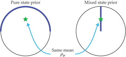
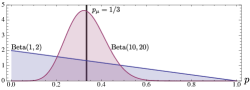
Here, we seek to use the default priors from Section III to construct a prior over states with that has a desired mean , and introduces little other information. The choice of the mean could be informed by, for example, experimental design or previous experimental estimates. Critically, a prior is not uniquely specified by the first moment of over , . Rather, the mean state only is a complete specification of observables measured against a state drawn from the prior. Indeed, different sets of assumptions can result in the same mean state, as illustrated in Figure 1. Thus, additional constraints are required to select an appropriate prior.
We also require that has support over all feasible states; for instance, those states of the appropriate dimension Shang et al. (2013), possibly subject to rank restrictions. By making this demand, our tomography procedure can recover from bad priors, given sufficient data; we will show the robustness of our algorithm in later in this section as well as in Section VI. Finally, we demand that our insightful priors can be sampled efficiently with the dimension of the state under consideration.
IV.1 Construction of Insightful Priors
To achieve the desiderata that all feasible states are supported, that we can sample efficiently, and that the prior mean is , we proceed in two steps. First, we sample from an fiducial prior i.e. . The sample from the fiducial prior is then transformed to a sample from the insightful prior under a generalized amplitude damping channel (GAD)
| (32) |
where is the damping parameter and is the fixed point of the map. For , the map is the identity channel, while for , the map damps to the mixed state . In our method is not a fixed number but is drawn from an ensemble described by the beta distribution, i.e. .
Thus to determine the mean of we must determine given and , that is
| (33) |
where on the second line we have used the fact that for priors that are fiducial, and on the third line we have used . Inverting this relationship tells one how to choose the fixed point of the channel (32) to obtain a given mean
| (34) |
Clearly we need more than the first moment to specify the prior; we must determine and to complete the specification. The first constraint on and comes from the positivity of , which is a valid state only if
| (35) |
where are the eigenvalues of . Thus, the minimum eigenvalue of partially constrains and by . In order to completely determine the parameters of the beta distribution, we adopt the principle that the action of the channel (32) should be minimized. We use this principle as an efficient heuristic motivated by analogy with maximum entropy methods. In other words, the insightful prior is as uninformative as possible given the constraint of the chosen mean, and with respect to a particular default prior.
We therefore choose to minimize the expected value , such that is the closest GAD-transformed distribution to with the given mean . This minimization gives
| (36) |
This construction naturally specializes to provide a procedure for estimating the bias of a coin, as discussed in Appendix D.
IV.2 Convexity and Robustness of Insightful Priors
Note that, because is in the support of all beta distributions, our prior ensures that its support is at least that of the given fiducial prior, . For the default priors listed in Section III, the prior constructed by our procedure has support over all states of the appropriate dimension. In general, the fiducial prior defines the states that we consider to be valid, as can be seen from the convexity of our construction.
That is, if is a convex combination over states in the support of the fiducial prior, then is the convex closure of . On the other hand, if lies outside of the support of the fiducial prior, then our algorithm chooses to lie outside as well, such that the support of the insightful prior is bigger than that of the convex closure of the fiducial support.
As our procedure preserves the support of the fiducial prior in both cases, our procedure also defines insightful priors for rebits and channels by using the real Ginibre and BCSZ priors as fiducial priors, respectively. In particular, using the BCSZ prior as the fiducial prior for a GAD-transformed distribution, we then obtain a prior that is insightful and is supported over all completely-positive and trace-preserving maps of a given dimension. Together with the Choi-Jamiołkowski isomorphism described in Appendix A, we can apply SMC to process tomography with little further effort.
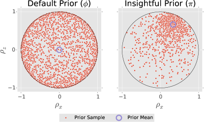
More exotic fiducial priors, such as distributions over stabilizer states or mundane states in the sense described by Veitch et al. (zero-mana) Veitch et al. (2014), can also be used, provided that they can be efficiently sampled and have the maximally-mixed state as their mean. For example, a prior that is insightful for mixed rebits is given in Figure 2.
Before proceeding, however, we note that our notion of a fiducial prior does not imply that such priors are uninformative— indeed, we have seen that they serve to define what states are considered valid at all. Indeed, as Wasserman states Wasserman (2013), “by definition, a prior represents information. So it should come as no surprise that a prior cannot represent lack of information.” As a further example, consider a prior over states of a given purity ; for a qubit, such states form a shell inside of the Bloch sphere. This prior conveys conveys information about what states are considered feasible at all, but still reports as its initial estimate that the state of interest is maximally mixed, i.e. it is fiducial, and can be used as input to our algorithm. Indeed, were one to do so, our algorithm would use this specification of what a feasible state is to define an insightful prior that is limited to a convex hull of the ball of states of purity no greater than and the desired mean state (provided , such that lies within the given purity ball). Taking the case as (that is, a -function prior supported only at the maximally-mixed state), the situation becomes more extreme, in that the insightful prior is then supported only on the line connecting the maximally-mixed state to . For this reason, the default priors given in Section III are chosen to have support over all states of a given dimension and rank, making them especially useful inputs to our algorithm.
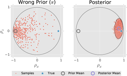
Finally, it is vital that the prior we have suggested is robust. In Figure 3 we choose the mean of our insightful prior to be almost orthogonal to the true state. After 300 random Pauli measurements, the posterior has support on the true state and the mean of the posterior is approximately the true state. Thus, even if the mean of the prior is woefully wrong our procedure is robust in that it provides a reliable estimate. This robustness to a bad initial prior requires additional data to be collected, such that useful prior information can accelerate experiments but will not, in general, lead to wrong conclusions. We explore this robustness further in Section VI.
V Tomographic State Tracking
In this section we use a generalization of particle filtering methods to track a stochastic processes. In the context of quantum state tomography, state-space methods allow us to characterize a stochastically-evolving source without having to ignore all previous data. We call the resulting method tomographic state tracking.
In particular we use the condensation algorithm, which interlaces Bayes updates with updates to move sequential Monte Carlo particles (using drift and diffusing of the particles), to follow a stochastic process Isard and Blake (1998). This technique has since been applied in a variety of other classical contexts Doucet et al. (2000); Jasra and Doucet (2009) as well as in quantum information Granade (2015a). Such methods, collectively known as state-space particle filtering, are useful for following the evolution of a stochastic process observed through a noisy measurement.
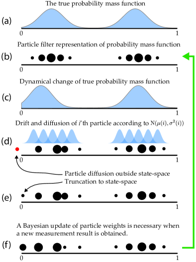
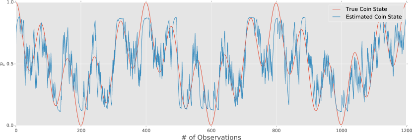
We now briefly explain the condensation algorithm, readers interested in further details are directed to the original paper Isard and Blake (1998). Consider Figure 4 which illustrates the condensation algorithm for tracking a coin with a dynamical bias . The current posterior of the coin bias, i.e. Figure 4(a), is given an SMC representation in Figure 4(b). In Figure 4(c), the true probability mass function changes— at this point, we step through the condensation algorithm to track this change. Each SMC particle is perturbed by a Gaussian. In particular, the th particle is perturbed by a Gaussian with mean and variance .
In keeping with the terminology used by Isard and Blake Isard and Blake (1998), the mean of the perturbation is termed the drift, and allows one to track deterministic evolution of a probability mass function; this becomes evident if for all . Similarly, the variance of the perturbation is termed diffusion and will allow the algorithm to track a stochastic process. As we will detail further below, both the drift and diffusion parameters can be learned online, such that we do not require them to be known a priori.
Sometimes the perturbation by the Gaussian will cause the particles to fall outside of the state space, in this case the unit interval, see e.g. Figure 4(d). In this situation, we modify the condensation algorithm to truncate particles to be valid probabilities, completing the Gaussian perturbation step, see Figure 4(e). Finally, we obtain the next datum and perform a Bayes update on the next datum. The final posterior approximation, Figure 4(f), then forms the new approximation (b) for the next diffusive update.
Interestingly, the condensation algorithm starts with a joint distribution over the parameters to be estimated. For the coin case, these are the bias , and the distribution parameters for drift and diffusion . Thus, when the Bayes update occurs the drift and diffusion parameters are updated as well, even though the likelihood does not explicitly depend on these parameters, which is referred to as co-evolution. It is this co-evolution that powers the tracking capabilities of the condensation algorithm.
As the learning of deterministic evolution of states is well-understood Schirmer and Oi (2010); Sergeevich et al. (2011); Granade et al. (2012b), we will suppose that the state under study is with respect to a frame that has already been well-characterized. Thus, the dominant remaining dynamics of the state under study are stochastic, such that we need not consider drift updates in our state-space model. Even with this assumption our model can still track deterministic evolution, however, provided that the diffusion is strong enough to include the true evolution with high probability (see Figure 5 for an example of tracking deterministic evolution with diffusion alone).
Concretely, we update particle by by first adding drift and diffusion terms to find a step to take in state-space, then truncating the negative eigenvalues of . For each particle , we let , where is a deterministic drift, and where each traceless component of is drawn from a Gaussian with standard deviation . As stated above, we work in a frame where the deterministic part has been taken out so that for all particles and for all time. The diffusion standard deviation is then taken to be a function of evolution time and the new model parameter , . This allows the evolution rate to “co-evolve” with the state model , as described above.
Diffusion is completed by finding the spectral decomposition of , then truncating and renormalizing. In particular, let . Then,
| (37) |
where is chosen such that . This truncation rule avoids expensive optimization to find the closest state consistent with a given drift and diffusion update , while still generalizing methods known to be effective and efficient for coin estimation.
In order to determine the limitations of state space tracking, we considered tracking a single tone cosine , where is a discrete time and is the time between samples. Recall that we are choosing not to include deterministic evolution (i.e. “drift”) in our model, thus the following observation only applies to purely diffusive tracking. We found the our algorithm could track a frequency up to . At higher frequencies, our approach failed to track the oscillatory behavior of , in that it would report for all time. This modality can be tested using model selection van Enk and Blume-Kohout (2013); Granade (2015a), such that more a appropriate algorithm can be used in that case. A more sophisticated, though less quantitative, analysis of this failure can be found in Appendix E.
VI Numerical Examples
We now show examples of Bayesian state and process tomography using sequential Monte Carlo, with priors that are respectively default and insightful. These examples were generated using QInfer Granade et al. (2012a).
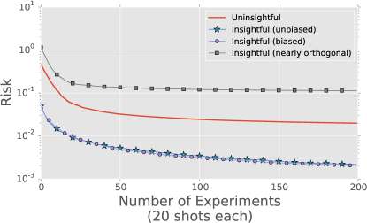
For state tomography, we demonstrate our methods by learning qutrit states, as shown in Figure 6. We demonstrate the performance of our algorithm in this case by reporting the risk, defined as the expected quadratic loss over repetitions of the algorithm,
| (38) |
We use each of a default, insightful and unbiased, and an insightful but biased prior. In all three cases, we draw the “true” states from the prior that matches the insightful and unbiased prior.
In Figure 6, we also verify that our method is robust for the qutrit example by considering an insightful prior whose mean is nearly orthogonal to the true state. Notably, in well over half of the 1200 trials considered in that case, QInfer reported that the algorithm was likely to fail, heralding the impact of the “bad” prior.
We then proceed to consider state-space quantum state tomography, as detailed in Section V. We demonstrate the performance of our state-space method in an animation, available online Granade et al. (2015b), also see Video VI for a snapshot.
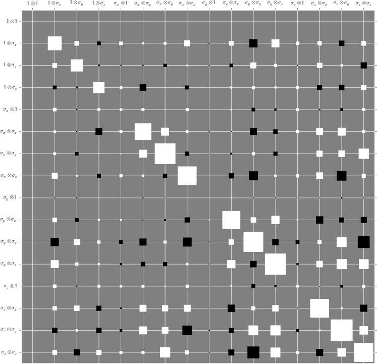
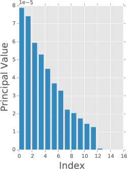
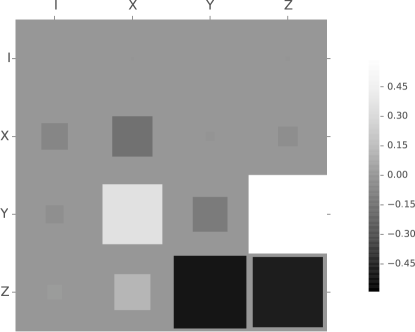
Finally, we demonstrate the application of our method to learning quantum channels acting on a qubit. In Figure 7, we show an example of a single simulated quantum process tomography experiment, where the true channel and the insightful prior (generated with a BCSZ fiducial prior) agree. The preparation and measurement settings are chosen to be elements of the Pauli basis. Specifically, 20% of the experiments use random Pauli preparation and measurements, while 80% of the experiment use settings that maximize out of 50 randomly proposed Pauli preparations and measurements; that is, adaptively chosen to overlap with the principal components of the current posterior. The resulting posterior distribution characterizes the uncertainty remaining about the “true” channel, as shown in Figure 8. In particular, we note the principal components of the posterior covariance matrix are themselves quantum maps which describe the directions of maximal uncertainty in the final posterior. For this example, our error is dominated by uncertainty about the contribution of the identity and Hadamard channels, as is made clear by visual inspection in Figure 8 (bottom right).
![[Uncaptioned image]](/html/1509.03770/assets/x7.png) \setfloatlink
\setfloatlink
https://goo.gl/mkibti This video demonstrates using tomographic state tracking to estimate a diffusing quantum state. Shown at left is the projection of the true state (star), the sequential Monte Carlo particle cloud (red dots), and covariance approximation to the 99% credible region (red circle) to the - plane. Shown at right is a Hinton diagram of the current posterior covariance matrix. At each time step, each element of the vectorized true state is perturbed by a Gaussian with mean 0 and standard deviation 0.0045, and then is truncated to lie within the space of valid quantum states. The prior over this diffusion rate is taken to be a log-normal distribution with mean 0.006. Each measurement consists of 25 shots along a random Pauli axis.
VII Conclusions
In this work, we have provided a new prior distribution over quantum states and channels that allows for including experimental insight, a software implementation for numerically approximating Bayesian tomography, and a method for tracking time-dependent states. Together, our advances make Bayesian quantum tomography practical for current and future experiments. In particular, our methods allow for exploiting well-known benefits of Bayesian methods, including credible region estimation, hyperparameterization and model selection.
We note, however, that our insightful prior on states and channels is completely specified by its first moment. An interesting and open problem would thus be to develop a prior on states and channels that is completely specified by its first and second moments.
Finally, with respect to the tomographic state tracking methods presented in Section V, it is worth noting that van Enk and Blume-Kohout van Enk and Blume-Kohout (2013) suggested that model selection could be used to determine if a source was drifting or diffusing. In this manuscript we have provided a way that allows one to track a source that is drifting or diffusing. It is also possible to combine the approaches and use model selection to determine when tracking is necessary or when a static model is sufficient as demonstrated by Granade Granade (2015a).
In short, with constructive methods for sampling from insightful priors, and with modern statistical methods, Bayesian state and process tomography are made practical for current experimental needs. This in turn allows us to explore new questions in tomography, and thus better characterize and diagnose quantum information processing systems.
Acknowledgements.
The authors acknowledge Sarah Kaiser, Chris Ferrie, Brendon Higgins, and Richard Küng for discussions. The authors acknowledge funding from Industry Canada, CERC, NSERC, the Province of Ontario, and the CFI is gratefully acknowledged. CG acknowledges Connor Jarvis for noticing an important typographical error. CG also acknowledges Ian Hincks, Nathan Wiebe, and Yuval Sanders for contributions to and testing of QInfer, as well as support from the US Army Research Office via grant numbers W911NF-14-1-0098 and W911NF-14-1-010. The authors would like to note independent related work by Faist and Renner Faist and Renner (2015) and by Struchalin et al. Struchalin et al. (2015).References
- Huszár and Houlsby (2012) F. Huszár and N. M. T. Houlsby, “Adaptive Bayesian quantum tomography,” Phys. Rev. A 85, 052120 (2012).
- Ferrie (2014a) C. Ferrie, “Quantum model averaging,” New Journal of Physics 16, 093035 (2014a).
- Cramer et al. (2010) M. Cramer, M. B. Plenio, S. T. Flammia, R. Somma, D. Gross, S. D. Bartlett, O. Landon-Cardinal, D. Poulin, and Y.-K. Liu, “Efficient quantum state tomography,” Nature Communications 1, 149 (2010).
- Wiebe et al. (2015) N. Wiebe, C. Granade, and D. G. Cory, “Quantum bootstrapping via compressed quantum Hamiltonian learning,” New Journal of Physics 17, 022005 (2015).
- Holzäpfel et al. (2015) M. Holzäpfel, T. Baumgratz, M. Cramer, and M. B. Plenio, “Scalable reconstruction of unitary processes and Hamiltonians,” Physical Review A 91, 042129 (2015).
- Newton and Young (1968) R. G. Newton and B.-I. Young, “Measurability of the spin density matrix,” Annals of Physics 49, 393 (1968).
- Band and Park (1970) W. Band and J. L. Park, “The empirical determination of quantum states,” Foundations of Physics 1, 133 (1970).
- Band and Park (1979) W. Band and J. L. Park, “Quantum state determination: Quorum for a particle in one dimension,” Am. J. Phys. 47, 188 (1979).
- Hradil (1997) Z. Hradil, “Quantum-state estimation,” Phys. Rev. 55, R1561 (1997).
- Christandl and Renner (2012) M. Christandl and R. Renner, “Reliable quantum state tomography,” Phys. Rev. Lett. 109, 120403 (2012).
- Blume-Kohout (2012) R. Blume-Kohout, “Robust error bars for quantum tomography,” (2012), 1202.5270 .
- Shang et al. (2013) J. Shang, H. K. Ng, A. Sehrawat, X. Li, and B.-G. Englert, “Optimal error regions for quantum state estimation,” New Journal of Physics 15, 123026 (2013).
- Guţă et al. (2012) M. Guţă, T. Kypraios, and I. Dryden, “Rank-based model selection for multiple ions quantum tomography,” New Journal of Physics 14, 105002 (2012).
- van Enk and Blume-Kohout (2013) S. J. van Enk and R. Blume-Kohout, “When quantum tomography goes wrong: drift of quantum sources and other errors,” New Journal of Physics 15, 025024 (2013).
- Blume-Kohout (2010a) R. Blume-Kohout, “Hedged maximum likelihood estimation,” (2010a), 1001.2029 .
- Gross et al. (2010) D. Gross, Y.-K. Liu, S. T. Flammia, S. Becker, and J. Eisert, “Quantum state tomography via compressed sensing,” Physical Review Letters 105, 150401 (2010).
- Flammia et al. (2012) S. T. Flammia, D. Gross, Y.-K. Liu, and J. Eisert, “Quantum tomography via compressed sensing: error bounds, sample complexity and efficient estimators,” New Journal of Physics 14, 095022 (2012).
- Jones (1991a) K. Jones, “Principles of quantum inference,” Ann. Phys. N.Y. 207, 140 (1991a).
- Jones (1991b) K. Jones, “Quantum limits to information about states for finite dimensional Hilbert space,” J. Phys. A: Math. Gen. 24, 121 (1991b).
- Jones (1994) K. Jones, “Fundamental limits upon the measurement of state-vectors,” Phys. Rev. A 50, 3682 (1994).
- Slater (1995) P. B. Slater, “Quantum coin-tossing in a Bayesian Jeffreys framework,” Physics Letters A 266, 66 (1995).
- Derka et al. (1996) R. Derka, V. Buzek, G. Adam, and P. L. Knight, “From quantum Bayesian inference to quantum tomography,” Journal of Fine Mechanics and Optics 11-12, 341 (1996).
- Bužek et al. (1998) V. Bužek, R. Derka, G. Adam, and P. L. Knight, “Reconstruction of quantum states of spin systems: From quantum Bayesian inference to quantum tomography,” Annals of Physics 266, 454 (1998).
- Schack et al. (2001) R. Schack, T. A. Brun, and C. M. Caves, “Quantum Bayes rule,” Phys. Rev. 64, 014305 (2001).
- Blume-Kohout and Hayden (2006) R. Blume-Kohout and P. Hayden, “Accurate quantum state estimation via “Keeping the experimeintalist honest”,” (2006), quantu-ph/0603116 .
- Blume-Kohout (2010b) R. Blume-Kohout, “Optimal, reliable estimation of quantum states,” New Journal of Physics 12, 043034 (2010b).
- Ferrie and Kueng (2015) C. Ferrie and R. Kueng, “Have you been using the wrong estimator? These guys bound average fidelity using this one weird trick von Neumann didn’t want you to know,” (2015), 1503.00677 .
- Kravtsov et al. (2013) K. S. Kravtsov, S. S. Straupe, I. V. Radchenko, N. M. T. Houlsby, F. Husz ar, and S. P. Kulik, “Experimental adaptive Bayesian tomography,” Physical Review A 87, 062122 (2013).
- Ferrie (2014b) C. Ferrie, “High posterior density ellipsoids of quantum states,” New Journal of Physics 16, 023006 (2014b).
- Wiebe et al. (2014a) N. Wiebe, C. Granade, C. Ferrie, and D. Cory, “Quantum Hamiltonian learning using imperfect quantum resources,” Physical Review A 89, 042314 (2014a).
- Struchalin et al. (2015) G. Struchalin, I. Pogorelov, S. Straupe, K. Kravtsov, I. Radchenko, and S. Kulik, “Experimental Adaptive Quantum Tomography of Two-Qubit States,” arXiv (2015).
- Doucet and Johansen (2009) A. Doucet and A. M. Johansen, “A tutorial on particle filtering and smoothing: Fifteen years later,” (Oxford: Oxford University Press) (2009).
- Doucet et al. (2000) A. Doucet, S. Godsill, and C. Andrieu, “On sequential Monte Carlo sampling methods for Bayesian filtering,” Statistics and Computing 10, 197 (2000).
- Audenaert and Scheel (2009) K. M. R. Audenaert and S. Scheel, “Quantum tomographic reconstruction with error bars: a Kalman filter approach,” New Journal of Physics 11, 023028 (2009).
- Ince et al. (2012) D. C. Ince, L. Hatton, and J. Graham-Cumming, “The case for open computer programs,” Nature 482, 485 (2012).
- Borot and Nadal (2012) G. Borot and C. Nadal, “Purity distribution for generalized random bures mixed states,” Journal of Physics A: Mathematical and Theoretical 45, 075209 (2012).
- Schwarz and van Enk (2011) L. Schwarz and S. J. van Enk, “Detecting the drift of quantum sources: Not the de Finetti theorem,” Physical Review Letters 106, 180501 (2011).
- Langford (2013) N. K. Langford, “Errors in quantum tomography: diagnosing systematic versus statistical errors,” New Journal of Physics 15, 035003 (2013).
- Shulman et al. (2014) M. D. Shulman, S. P. Harvey, J. M. Nichol, S. D. Bartlett, A. C. Doherty, V. Umansky, and A. Yacoby, “Suppressing qubit dephasing using real-time Hamiltonian estimation,” Nature Communications 5, 5156 (2014).
- Fogarty et al. (2015) M. A. Fogarty, M. Veldhorst, R. Harper, C. H. Yang, S. D. Bartlett, S. T. Flammia, and A. S. Dzurak, “Nonexponential fidelity decay in randomized benchmarking with low-frequency noise,” Physical Review A 92, 022326 (2015).
- Granade (2015a) C. E. Granade, Characterization, Verification and Control for Large Quantum Systems, Ph.D. thesis (2015a).
- Blume-Kohout et al. (2015) R. Blume-Kohout, J. K. Gamble, E. Nielsen, P. Maunz, T. Scholten, and K. Rudinger, Turbocharging Quantum Tomography., Tech. Rep. (Sandia National Laboratories (SNL-NM), Albuquerque, NM (United States), 2015).
- Granade et al. (2012a) C. Granade, C. Ferrie, et al., QInfer: Library for Statistical Inference in Quantum Information (2012).
- Johansson et al. (2013) J. R. Johansson, P. D. Nation, and F. Nori, “QuTiP 2: A Python framework for the dynamics of open quantum systems,” Computer Physics Communications 184, 1234 (2013), arXiv:1211.6518 [quant-ph].
- Casagrande and Granade (2013) S. Casagrande and C. Granade, InstrumentKit: Python package for interacting with laboratory equipment (2013).
- Banerjee et al. (2005) A. Banerjee, X. Guo, and H. Wang, “On the optimality of conditional expectation as a Bregman predictor,” IEEE Transactions on Information Theory 51, 2664 (2005).
- Note (1) This definition of the quadratic loss follows from the typical definition by interpreting the scale matrix as a superoperator.
- Granade et al. (2012b) C. E. Granade, C. Ferrie, N. Wiebe, and D. G. Cory, “Robust online Hamiltonian learning,” New Journal of Physics 14, 103013 (2012b).
- (49) N. Wiebe, C. Granade, A. Kapoor, and K. M. Svore, (in preparation).
- Doucet and Johansen (2011) A. Doucet and A. M. Johansen, A tutorial on particle filtering and smoothing: fifteen years later (2011).
- Wasserman (2013) L. Wasserman, “LOST CAUSES IN STATISTICS II: Noninformative Priors,” (2013).
- Osipov et al. (2010) V. A. Osipov, H.-J. Sommers, and K. Zyczkowski, “Random Bures mixed states and the distribution of their purity,” J. Phys. A: Math. Theor. 43, 055302 (2010).
- Zyczkowski and Sommers (2001) K. Zyczkowski and H.-J. Sommers, “Induced measures in the space of mixed quantum states,” Journal of Physics A: Mathematical and General 34, 7111 (2001).
- Mezzadri (2007) F. Mezzadri, “How to generate random matrices from the classical compact groups,” Notices of the American Mathematical Society 54, 592 (2007).
- Note (2) More generally, Osipov et al. Osipov et al. (2010) show that by linearly interpolating between and in (29), one obtains a continuous family of distributions with the Hilbert-Schmidt and Bures ensembles as its extrema.
- Bruzda et al. (2009) W. Bruzda, V. Cappellini, H.-J. Sommers, and K. Źyczkowski, “Random quantum operations,” Physics Letters A 373, 320 (2009).
- Veitch et al. (2014) V. Veitch, S. A. H. Mousavian, D. Gottesman, and J. Emerson, “The resource theory of stabilizer quantum computation,” New Journal of Physics 16, 013009 (2014).
- Granade et al. (2015a) C. Granade, J. Combes, and D. G. Cory, “Practical Bayesian tomography supplementary video: Recovery from “bad” priors,” https://goo.gl/gpb94w (2015a).
- Isard and Blake (1998) M. Isard and A. Blake, “CONDENSATION–conditional density propagation for visual tracking,” International Journal of Computer Vision 29, 5 (1998).
- Jasra and Doucet (2009) A. Jasra and A. Doucet, “Sequential Monte Carlo methods for diffusion processes,” Proceedings of The Royal Society A: Mathematical, Physical and Engineering Sciences 465, 3709 (2009).
- Schirmer and Oi (2010) S. G. Schirmer and D. K. L. Oi, “Quantum system identification by Bayesian analysis of noisy data: Beyond Hamiltonian tomography,” Laser Physics 20, 1203 (2010).
- Sergeevich et al. (2011) A. Sergeevich, A. Chandran, J. Combes, S. D. Bartlett, and H. M. Wiseman, “Characterization of a qubit Hamiltonian using adaptive measurements in a fixed basis,” Physical Review A 84, 052315 (2011).
- Granade et al. (2015b) C. Granade, J. Combes, and D. G. Cory, “Practical Bayesian tomography supplementary video: State-space state tomography,” https://goo.gl/mkibti (2015b).
- Faist and Renner (2015) P. Faist and R. Renner, “Practical, Reliable Error Bars in Quantum Tomography,” arXiv:1509.06763 [quant-ph] (2015), arXiv: 1509.06763.
- Chuang and Nielsen (1997) I. L. Chuang and M. A. Nielsen, “Prescription for experimental determination of the dynamics of a quantum black box,” Journal of Modern Optics 44, 2455 (1997).
- Choi (1975) M.-D. Choi, “Completely positive linear maps on complex matrices,” Linear Algebra and its Applications 10, 285 (1975).
- Jamiołkowski (1972) A. Jamiołkowski, “Linear transformations which preserve trace and positive semidefiniteness of operators,” Reports on Mathematical Physics 3, 275 (1972).
- Wood et al. (2015) C. J. Wood, J. D. Biamonte, and D. G. Cory, “Tensor networks and graphical calculus for open quantum systems,” Quantum Information and Computation 15, 0579 (2015), arXiv: 1111.6950.
- Wood (2015) C. Wood, Initialization and characterization of open quantum systems, Ph.D. thesis (2015).
- Ringbauer et al. (2014) M. Ringbauer, C. J. Wood, K. Modi, A. Gilchrist, A. G. White, and A. Fedrizzi, “Characterizing quantum dynamics with initial system-environment correlations,” arXiv:1410.5826 [quant-ph] (2014), arXiv: 1410.5826.
- Altepeter et al. (2003) J. B. Altepeter, D. Branning, E. Jeffrey, T. C. Wei, P. G. Kwiat, R. T. Thew, J. L. O’Brien, M. A. Nielsen, and A. G. White, “Ancilla-assisted quantum process tomography,” Physical Review Letters 90, 193601 (2003).
- Watrous (2013) J. Watrous, “CS 766: Theory of quantum information,” (lecture notes) (2013).
- Granade (2015b) C. Granade, “Robust online Hamiltonian learning: Multi- model resampling,” https://goo.gl/CR9Dtr (2015b).
- Stenberg et al. (2014) M. P. Stenberg, Y. R. Sanders, and F. K. Wilhelm, “Efficient estimation of resonant coupling between quantum systems,” Physical Review Letters 113, 210404 (2014).
- Wiebe et al. (2014b) N. Wiebe, C. Granade, C. Ferrie, and D. Cory, “Hamiltonian learning and certification using quantum resources,” Physical Review Letters 112, 190501 (2014b).
- Svensson (2013) A. Svensson, “The particle filter explained without equations,” https://goo.gl/VjZJVm (2013).
Appendix A Choi-Jamiołkowski Isomorphism and QPT
In order to interpret (1a) as specifying probabilities for quantum process tomography Chuang and Nielsen (1997) as well as state tomography, we use the Choi-Jamiołkowski isomorphism and represent a hypothesis about the channel as a state
| (39) |
The formalism of using the Choi-Jamiołkowski isomorphism Choi (1975); Jamiołkowski (1972) to describe open quantum processes has also been recently detailed in detail by Wood et al. Wood et al. (2015) using tensor network diagrams with particular regard to quantum tomography and its generalizations Wood (2015); Ringbauer et al. (2014).
In the case that quantum process tomography is carried out by ancilla-assisted process tomography Altepeter et al. (2003), we are done, as is, up to normalization, the state used in AAPT. On the other hand, we can also use that for any linear operator , to represent preparation followed by evolution under and measurement as a measurement of Watrous (2013). In particular, suppose that a QPT experiment is performed in which each observation consists of a measurement effect and a preparation ,
| (40a) | ||||
| (40b) | ||||
| (40c) | ||||
| (40d) | ||||
where and . This now has the form of a measurement being made on a state , such that (1a) completely describes the outcomes of both in-place and ancilla-assisted QPT experiments. Though we used the column-stacking basis to derive this equivalence, implicitly defining a convention for the Choi state, we can insert a unitary operator on the space of vectorized operators to observe that (40d) is not dependent on the choice of basis.
The likelihood after measurements is
| (41) |
where is the string of measurement results and is the observation of the ’th generalized measurement. Note that (41) is of the same form as (1a), such that quantum process tomography can be treated as a special case of quantum state tomography, provided that we use an appropriate fiducial prior.
Appendix B Review of Sequential Monte Carlo
The purpose of this appendix is to provide a minimal summary and point the interested reader to the relevent literature on the particle filtering and sequential Monte Carlo (SMC) algorithms as applied to Bayesian inference. There is a wealth of information in the references that need not be reproduced here.
The basic idea of SMC is to approximate a distribution over some parameters conditioned on the th data , i.e. . The approximation uses a weighted sum of delta-functions, specifically
| (42) |
where the objects are called particles and is the weight of the th particle. Here (42) should be compared to (26) of the main text; where we suppressed many technical and notational details. As the number of particles increases the quality of the approximation improves. The initial particles are chosen by sampling the prior distribution over , and are taken to have uniform weight.
The next step is to update the posterior distribution given new datum say the th data is . Then using the likelihood function the particle weights are updated from the previous weights () using
| (43) |
Clearly, the particle weights after this update need to renormalized such that .
As updates proceed, the concentration of weights on the most plausible particles causes the distribution to be samples by a much smaller number of effective particles, as measured by the effective sample size . Thus, periodically particle locations have to be perturbed and the weights reset to uniform, restoring numerical stability. This is called resampling. A video demonstrating the Bayesian update and resampling steps for a simple Hamiltonian learning problem is available online Granade (2015b).
In the remainder of this appendix we provide references which can be used to obtained more details on SMC. Doucet et al. have provided a more through review from the perspective of classical statistics Doucet and Johansen (2009, 2011). In the quantum domain summaries of the SMC algorithm can be found in references Granade et al. (2012b); Ferrie (2014b); Stenberg et al. (2014); Wiebe et al. (2014b, a, 2015). Finally, Svensson has provided a useful video tutorial illustrating the application of particle filters in a simplified radar application Svensson (2013).
For our application (quantum tomography), Huszár and Houlsby Huszár and Houlsby (2012) and by Ferrie Ferrie (2014a) suggested SMC as numerical tool for implementing (5). Of particular interest is Ferrie’s recent work on tomographic region estimators with SMC Ferrie (2014b). Ref. Granade (2015a) has provided a summary of recent applications in quantum information.
Appendix C Sampling Default Priors
In this Appendix we review the algorithms necessary to sample from default priors, provided by References Zyczkowski and Sommers (2001); Mezzadri (2007); Osipov et al. (2010); Bruzda et al. (2009).
Appendix D GADFLI Prior for Coins
A prior distribution over the bias of a coin is a special case of a qubit and rebit prior. It corresponds to a prior over one axis of the Bloch sphere. Without loss of generality, we will take that axis to be the -axis, such that the density operator for a coin is given by
| (48) |
where is the -axis coordinate on the Bloch sphere at which the coin state is positioned.
Given the result of a coin toss , we assign a likelihood for that outcome conditioned on the coin as
| (49) |
where the probability of heads is . Using the density operator definition of a coin, we define that the minimum eigenvalue of a coin is .
We draw samples of the coin state from our GAD prior by first choosing and to be sampled from a fiducial prior such that . Through the rest of this example, we use . The GAD-prior sample is obtained by transitioning with a linear function given by
| (50) |
The expectation over this GAD prior then gives the Bayesian mean estimator before any data is collected. Using that is fiducial (has mean ) and that , we find that
| (51) |
and . Inverting, we find that the fixed point needed to guarantee that the prior mean is is given by
| (52) |
which is analogus to equation (34). In order for to be a valid coin, this constrains
| (53) |
We find and consistent with this condition and such that the mean
| (54) |
is minimized. This represents that the GAD channel used to define samples does as little as possible to transform fiducial (uniform) samples to our prior. Minimizing subject to the constraints that and , we obtain that
| (55) |
We can write this in terms of to obtain the final GAD-prior condition,
| (56) |
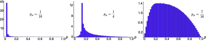
which should be compared to (36). Using this condition, we obtain the coin priors shown in Figure 10.
Appendix E An estimate of the tracking frequency
We now give an order of magnitude estimate for maximum frequency that is “smoothly” trackable by our algorithm. It is possible our algorithm can track higher frequencies but the evolution is likely to be fairly discontinuous.
Our estimate for the tracking frequency comes from sampling arguments in tracking a bias of a coin, with probability for heads. We will assume the coin’s bias changes from to where . The question is how quickly can we detect such a change, i.e. how many equally spaced in time samples does it take to notice the difference of .
We must specify an error tolerance––for our sensing protocol and a confidence interval––for our estimate of . It turns out if we use the trace distance between two coins and then . These two specifications will in turn (approximately) determine the number of samples required and therefore the bandwidth of our tracking protocol. We choose which corresponds to a level of confidence for our estimator and the maximum acceptable error . Using the standard deviation of the Bernouli distribution , we have . The largest standard deviation (worst case) is when this gives . Rearranging for gives . To obtain this many samples we must measure for a time , where is the time between measurements. Thus is effectively the time between our samples of . Naïve arguments from the Nyquist-Shannon sampling theorem imply that we can not determine frequency components of greater than , which is called the is detection frequency bandwidth. The implication is we can track, for example, .
Appendix F QInfer Tomography Tutorial
In this Appendix, we demonstrate the use of QInfer for Bayesian state and process tomography. In particular, we show how to estimate states and channels given data synthesized from a description of a true state, and discuss how to obtain region estimates, covariance superoperators and other useful functions of tomography posteriors. We then discuss how to apply these techniques in experimental systems.
The tomography implementation in QInfer is based on QuTiP and NumPy, so we start by importing everything here.
In [1]: import numpy as np import qutip as qt import qinfer as qi
As a first step, we define a basis for performing tomography; the choice of basis is largely arbitrary, but depending on the experiment, some bases may be more or less convienent. Here, we focus on the example of the single-qubit Pauli basis .
In [2]: basis = qi.tomography.pauli_basis(1) display(basis)
<TomographyBasis dims=[2] at 362504488>
We will get a lot of use out of the Pauli basis, so we also define some useful shorthand.
In [3]: I, X, Y, Z = qt.qeye(2), qt.sigmax(), qt.sigmay(), qt.sigmaz()
Basis objects are responsible for converting between QuTiP’s rich Qobj format and the unstructured model parameter representation used by QInfer.
In [4]: display(basis.state_to_modelparams(I / 2 + X / 2))
array([ 0.70710678, 0.70710678, 0. , 0. ])
In [5]: display(basis.modelparams_to_state(np.array([1, 0, 0, 1]) / np.sqrt(2)))
Quantum object: dims = [[2], [2]], shape = [2, 2], type = oper, isherm = True
Having defined a basis, we then define the core object describing a tomography experiment, the model. In QInfer, models encapsulate the likelihood function, experimental parameters and other useful metadata about the experimental properties being estimated. In our case, we use TomographyModel to describe the single-shot experiment, and BinomialModel to describe batches of the single-shot experiment.
In [6]: model = qi.BinomialModel(qi.tomography.TomographyModel(basis)) display(model)
<qinfer.derived_models.BinomialModel at 0x159b6048>
A Model defines a vector of model parameters; for a single qubit TomographyModel, this is a vector of length 4, each describing a different element of the Hermitian operator basis. Each Model also defines experiment parameters as a NumPy record array. A record then describes a single measurement of the model.
In [7]: display(model.expparams_dtype)
[(’meas’, float, 4), (’n_meas’, ’uint’)]
In this case, the experiment parameters record has two fields: meas and n_meas. The first is a vector of four floats corresponding to . The second is an unsigned integer (uint) describing how many times that measurement is performed. For instance, measuring 40 times is given by the array:
In [8]: expparams = np.array([ # Each tuple, marked with (), defines a single record. ( # Within each tuple, fields are separated by commas. # The fields follow in the order given by the model, # so the first field is meas, a length-4 vector. [1 / np.sqrt(2), 0, 0, 1 / np.sqrt(2)], # The second field is then the number of measurements. 40 ) ], # We finish building the array by passing along the right data\ # type to NumPy. This is somwhat of a QInfer idiom. dtype=model.expparams_dtype) display(expparams)
array([([0.7071067811865475, 0.0, 0.0, 0.7071067811865475], 40L)],
      dtype=[(’meas’, ’<f8’, (4,)), (’n_meas’, ’<u4’)])
The fields of a record array can be obtained by indexing. For instance, the ['meas'] field is then a array, with the first index allowing for a sequence of measurements to be described at once.
In [9]: display(expparams[’meas’])
array([[ 0.70710678, 0. , 0. , 0.70710678]])
Note that by convention, meas is normalized to .
Often, we will not construct experiments directly, but will instead rely on QInfer’s heuristics (described below). In any case, once we have a model, the next step is to create a prior. QInfer comes with several useful fiducial priors, as well as insightful priors constructed from amplitude damping channels. For instance, to create a Hilbert-Schmidt uniform prior constrained to rebits, we use the GinibreReditDistribution:
In [10]: fiducial_prior = qi.tomography.GinibreReditDistribution(basis)
In [11]: qi.tomography.plotting_tools.plot_rebit_prior(fiducial_prior, rebit_axes=[1, 3])
Here, we have told QInfer that we wish to treat and as our rebit axes using the rebit_axes=[1, 3] argument.
Insightful priors can be constructed by specifying a fiducial prior and a QuTiP Qobj representing the desired mean.
In [12]: prior_mean = (I + (2/3) * Z + (1/3) * X) / 2 display(prior_mean)
Quantum object: dims = [[2], [2]], shape = [2, 2], type = oper, isherm = True
In [13]: prior = qi.tomography.GADFLIDistribution(fiducial_prior, prior_mean)
In [14]: qi.tomography.plotting_tools.plot_rebit_prior(prior, rebit_axes=[1, 3])
Having constructed a prior and a model, we can now continue to perform Bayesian inference using SMC. We demonstrate using the true state with the prior mean .
In [15]: basis = qi.tomography.pauli_basis(1) model = qi.BinomialModel(qi.tomography.TomographyModel(basis)) true_state = basis.state_to_modelparams( I / 2 + (2 / 3) * Z / 2 )[np.newaxis, :] fiducial_prior = qi.tomography.GinibreReditDistribution(basis) prior = qi.tomography.GADFLIDistribution(fiducial_prior, I / 2 + (4 / 5) * Z / 2 + (1 / 7) * X / 2 )
In [16]: qi.tomography.plotting_tools.plot_rebit_prior(prior, true_state=true_state, rebit_axes=[1, 3])
The updater and heuristic classes track the posterior and the random-measurement experiment design, respectively.
In [17]: updater = qi.smc.SMCUpdater(model, 2000, prior) heuristic = qi.tomography.RandomPauliHeuristic(updater, other_fields={’n_meas’: 40})
We synthesize data for the true state, then feed it into the updater in order to obtain our final posterior.
In [18]: for idx_exp in xrange(50): experiment = heuristic() datum = model.simulate_experiment(true_state, experiment) updater.update(datum, experiment)
In [19]: plt.figure(figsize=(10, 10)) qi.tomography.plotting_tools.plot_rebit_posterior( updater, prior, true_state, rebit_axes=[1, 3] )
We can use our tomography basis object to read out the estimated final state as a QuTiP Qobj.
In [20]: est_mean = basis.modelparams_to_state(updater.est_mean()) display(est_mean)
Quantum object: dims = [[2], [2]], shape = [2, 2], type = oper, isherm = True
As discussed in the main text, the posterior can also be described by the covariance superoperator . We demonstrate by showing the Choi matrix .
In [21]: cov_superop = basis.covariance_mtx_to_superop(updater.est_covariance_mtx()) display(qt.to_choi(cov_superop)) display(Latex(r"$\|\Sigma\rho\|_{{\Tr}} = {:0.4f}$".format(cov_superop.norm(’tr’))))
Quantum object: dims = [[[2], [2]], [[2], [2]]], shape = [4, 4], type = super, isherm = True, superrep = choi
Here, we use the Hinton diagram plotting functionality provided by QuTiP to depict the covariance in each observable that we obtain from the posterior.
In [22]: display(qt.visualization.hinton(cov_superop))
(<matplotlib.figure.Figure at 0x18218a20>,
 <matplotlib.axes._subplots.AxesSubplot at 0x18209f98>)