A generalized fidelity amplitude for open systems

Abstract

We consider a central system which is coupled via dephasing to an open system, i.e. an intermediate system which in turn is coupled to another environment. Considering intermediate and far environment as one composite system, the coherences in the central system are given in the form of fidelity amplitudes for a certain perturbed echo dynamics in the composite environment. On the basis of the Born-Markov approximation, we derive a master equation for the reduction of that dynamics to the intermediate system alone. In distinction to an earlier paper [arXiv: 1502.04143 (2015)] where we discussed the stabilizing effect of the far environment on the decoherence in the central system, we focus here on the possibility to use the measurable coherences in the central system for probing the open quantum dynamics in the intermediate system. We illustrate our results for the case of chaotic dynamics in the near environment, where we compare random matrix simulations with our analytical result.

Keywords

Quantum Loschmidt echo, Fidelity, Open quantum system, Master equation, Random matrix theory

1 Introduction

Loss of fidelity and decoherence are the twin obstacles to successful applications of quantum information devices. Theoreticians like to consider the two separately, while in practical situations both will have destructive effects on quantum information flow. In this spirit it is important to propose a functional definition for the fidelity or better the fidelity amplitude of an open system. To achieve this we shall build on previous work. Almost 20 years ago a measurement of the fidelity amplitude in a quantum system was proposed [1], though the word itself was not mentioned. A more detailed presentation for a kicked rotor followed years later [2], simultaneously with an extensive discussion of the theoretical framework [3]. The experiment for the kicked rotor was performed successfully in Ref. [4]. The basic idea is that pure dephasing between a qubit and some system will cause the off diagonal elements or coherences of the density matrix of a pure superposition state of the qubit decay like the fidelity amplitude of the remaining system. Our proposition is to follow exactly the same reasoning in the case where the remaining system is open, and thus interpret the decaying coherences as a generalized fidelity amplitude of the intermediate system.

For this purpose we have to consider a situation discussed in a previous paper [5], where a central system coupled to two nested environments is analyzed to determine the effect of a far environment on the coherence of a central system not interacting directly with the far environment. The intermediate system or “near environment” would then be the open system we are analyzing using the qubit as a probe and as the source of the perturbation causing the fidelity decay in the absence of the far environment.

Our paper will thus fulfill a double purpose: On the one hand we shall introduce a generalized fidelity amplitude and study its behaviour in a “quantum chaotic” setting. On the other we shall deepen the understanding of the stabilizing effect on the central system of the coupling of the near environment to a far environment. Note that in a previous paper [5] we introduced pure dephasing between the central system and the near environment, as a simplifying approximation to facilitate calculations, but for the present context this is an essential feature needed in order to establish the relation to fidelity decay of a closed system.

Considering near and far environment as one closed system, the fidelity amplitude may be expressed as the expectation value of an echo operator [6], which describes the forward and backward evolution of an initial state with somewhat different Hamiltonians. In the present paper we shall derive a master equation which describes this echo dynamics reduced to the near environment alone. This master equation has the typical structure of master equations of Kosakowski-Sudarshan-Lindblad form [7, 8] (henceforth referred to as Lindblad equation) and reduce to Lindblad form when the coupling to the central system becomes zero.

We then consider the random matrix model already used in Ref. [5]. In that case, the master equation becomes very simple, and allows to obtain a closed integral equation for the generalized fidelity amplitude. We compare the solution of the integral equation with the generalized fidelity amplitude obtained from numerical simulations, and thereby show that the new integral equation applies for a very broad range of coupling strengths between near and far environment. While the random matrix model used here, is much simpler than the one used in Ref. [5], its effect on the fidelity amplitude is typically indistinguishable.

In the next section we shall fix notations and obtain the general master equation for describing the reduced echo dynamics in the near environment. At the end of this section, we derive the master equation for the random matrix model, which is largely equivalent to the model considered in [5]. In Sec. 3 we compare the generalized fidelity amplitude obtained from the new integral equation with numerical simulations, and in the last section we draw conclusions.

2 Model

In this section we describe the model in general. The full system consists of three parts, the central system, the near environment and a far environment. In the following section (Sec. 2.1) we start from a Hamiltonian formulation, and perform partial traces in order to obtain the reduced dynamics either in the central system or in the near environment. Assuming a dephasing coupling between central system and near environment, we can obtain the temporal evolution of the reduced density matrix in the central system, in terms of an asymmetric unitary evolution (perturbed echo dynamics) in the composite environment. In Sec. 2.2 we then use the standard Born-Markov approximation to trace out the far environment, and thereby arrive at a master equation for the reduced echo dynamics in the near environment alone.

2.1 Hamiltonian formulation

For the coupling between central system and near environment, we assume that it is of the dephasing type, i.e. that it is given by a single product term, where the factor acting in the central system commutes with the Hamiltonian describing the dynamics in the central system. Thus, the Hamiltonian for this part is given as

$$H_{\rm c,e}=h_{\rm c}\otimes\mathbbm{1}_{\rm e}+\mathbbm{1}_{\rm c}\otimes H_{\rm e}+v_{\rm c}\otimes V_{\rm e}\;,\quad\text{where}\quad[h_{\rm c},v_{\rm c}]=0\;.$$ (1)

This leads to the following expression for the time evolution of the reduced density matrix in the central system [1, 3]

$$\varrho_{\rm c}(t)={\rm tr}_{\rm e}\big{[}\,{\rm e}^{-{\rm i}H_{\rm c,e}t/\hbar}\,\varrho_{\rm c}(0)\otimes\varrho_{\rm e}\,{\rm e}^{{\rm i}H_{\rm c,e}t/\hbar}\,\big{]}\;,$$ (2)

which yields for its individual matrix elements (coherences)

$$\varrho^{\rm c}_{jk}(t)=\varrho^{\rm c}_{jk}(0)\;{\rm e}^{-{\rm i}(\varepsilon_{j}-\varepsilon_{k})/\hbar}\;f_{\lambda}(t)\;,\qquad f_{\lambda}(t)={\rm tr}\big{[}\,{\rm e}^{-{\rm i}H_{\lambda}t/\hbar}\,\varrho_{\rm e}\,{\rm e}^{{\rm i}H_{0}t/\hbar}\,\big{]}\;.$$ (3)

Here, we use the common eigenbasis of $h_{\rm c}$ and $v_{\rm c}$ to express $\varrho_{\rm c}(t)$, and therefore the energies $\varepsilon_{j}$ and $\varepsilon_{k}$ are simply the corresponding eigenvalues of $h_{\rm c}$. In what follows we will focus on only one such matrix element, and therefore suppress the indices $j,k$ from now on. We thus set

$$H_{\lambda}=H_{\rm e}+\lambda\;V_{\rm e}=H_{\rm e}+\nu_{j}\,V_{\rm e}\quad\text{and}\quad H_{0}=H_{\rm e}+\nu_{k}\,V_{\rm e}\;,$$ (4)

which implies that $\lambda=\nu_{j}-\nu_{k}$. This shows that under dephasing coupling, the decoherence in the central system is given by the decay of the fidelity or Lohschmidt echo in the near environment. Turning the argument the other way around, this shows that it is possible to measure fidelity amplitudes, by coupling the system of interest (i.e. the near environment) to a probe system, which at the same time provides the perturbation. Such experiments have been proposed and recently realized in different settings using atom interferometry [1, 2, 9, 4].

Including the far environment

We now extend the model to include a far environment. We assume the far environment to be as simple as possible and that it allows to be taken into account implicitly in the form of a quantum master equation. Hence, we write for the Hamiltonian of the full tripartite system:

$$H_{\lambda,\Gamma}=H_{\rm c,e}\otimes\mathbbm{1}_{\rm f}+\mathbbm{1}_{\rm c}\otimes\;\big{(}\,\mathbbm{1}_{\rm e}\otimes H_{\rm f}+\gamma\;V^{\prime}_{\rm e}\otimes V_{\rm f}\,\big{)}\;,$$ (5)

where $\Gamma=2\pi\,N_{\rm e}\,\gamma^{2}/(\hbar d_{\rm f})$. Here, $V^{\prime}_{\rm e}$ and $V_{\rm f}$ are normalized in such a way that $\gamma^{2}$ gives the magnitude squared of a typical matrix element of the coupling term between near and far environment. With $d_{\rm f}$ being the average level spacing (i.e. the inverse level density) in the spectrum of $H_{\rm f}$, we see that $\Gamma$ is just $N_{\rm e}$ times the corresponding Fermi golden rule transition rate [10, 11]. Finally, $\Gamma$ itself is related to the decoherence rate for a superposition of $N_{\rm e}$ states in the near environment. In the simplest case (see Sec. 3), $2\Gamma$ is precisely the decay rate of the purity in the intermediate system, in the case where the coupling to the central system is set to zero.

Within the Hamiltonian model described by $H_{\lambda,\Gamma}$, the coupling to the far environment requires the following modification to the expression for the fidelity amplitude given in Eq. (3):

$$f_{\lambda,\Gamma}(t)={\rm tr}_{\rm e,f}\big{[}\,{\rm e}^{-{\rm i}H_{\lambda,\Gamma}\,t/\hbar}\;\varrho_{\rm e,f}(0)\;{\rm e}^{{\rm i}H_{0,\Gamma}\,t/\hbar}\,\big{]}\;.$$ (6)

Differing from the standard formalism, the unitary operators on the left and on the right hand side of the initial state are different. This is why the trace may decrease in time, leading to the loss of coherence for superposition states in the central system [5].

2.2 Master equation for the echo dynamics

We follow the standard derivation of the Born-Markov approximation, e.g. Sec. 3.3 of Ref. [12]. However, due to the asymmetric unitary transformation implied in Eq. (6), the following derivation requires some care. Let us denote the solution in the Hilbert space of near and far environment as

$$\varrho_{\rm e,f}(t)={\rm e}^{-{\rm i}H_{\lambda,\Gamma}\,t/\hbar}\;\varrho_{\rm e,f}\;{\rm e}^{{\rm i}H_{0,\Gamma}\,t/\hbar}={\rm e}^{-{\rm i}H_{\lambda,0}\,t/\hbar}\;X(t)\;{\rm e}^{{\rm i}H_{0,0}\,t/\hbar}\;,$$ (7)

and thereby introduce $X(t)$ as the solution in the interaction picture with respect to the coupling between near and far environment. From the von Neumann equation for $\varrho_{\rm e,f}(t)$,

$${\rm i}\hbar\,\partial_{t}\,\varrho_{\rm e,f}(t)=H_{\lambda,\Gamma}\;\varrho_{\rm e,f}(t)-\varrho_{\rm e,f}(t)\;H_{0,\Gamma}\;,$$ (8)

we obtain

$${\rm i}\hbar\,\partial_{t}\,X(t)=\gamma\;\big{[}\,\tilde{V}_{\lambda}(t)\;X(t)-X(t)\;\tilde{V}_{0}(t)\,\big{]}\;,\qquad\tilde{V}_{\lambda}(t)={\rm e}^{{\rm i}H_{\lambda,0}\,t/\hbar}\;V_{\rm e}^{\prime}\otimes V_{\rm f}\;{\rm e}^{{\rm i}H_{0,0}\,t/\hbar}\;.$$ (9)

The aim of the Born-Markov approximation (to be worked out next) consists in obtaining a master equation for the reduced dynamics in the near environment alone. That is, an evolution equation for $\varrho_{\rm e}(t)={\rm tr}_{\rm f}\big{[}\varrho_{\rm e,f}(t)\,\big{]}$ which may not be considered a real quantum state, since for the reasons discussed above, $\varrho_{\rm e}(t)$ is neither Hermitian nor trace-preserving. This quasi-density operator is related to $X(t)$ as follows:

$$\varrho_{\rm e}(t) ={\rm tr}_{\rm f}\big{[}{\rm e}^{-{\rm i}H_{\lambda,0}t/\hbar}\;X(t)\;{\rm e}^{-{\rm i}H_{0,0}t/\hbar}\,\big{]}={\rm tr}_{\rm f}\big{[}U_{\lambda}(t)\otimes U_{\rm f}(t)\;X(t)\;U_{0}(t)^{\dagger}\otimes U_{\rm f}(t)^{\dagger}\,\big{]}\;,$$ (10)

where $U_{\lambda}(t)={\rm e}^{-{\rm i}H_{\lambda}t/\hbar}$ and $U_{\rm f}(t)={\rm e}^{-{\rm i}H_{\rm f}t/\hbar}$, since $H_{\lambda,0}$ and $H_{0,0}$ are both separable operators. Using the identities

$${\rm tr}_{\rm f}\big{[}A\otimes\mathbbm{1}\;X\,\big{]}=A\;{\rm tr}_{\rm f}[X\,]\;,\quad{\rm tr}_{\rm f}\big{[}X\;B\otimes\mathbbm{1}\,\big{]}={\rm tr}_{\rm f}[X\,]\;B$$

$${\rm tr}_{\rm f}\big{[}\mathbbm{1}\otimes A\;X\,\big{]}={\rm tr}_{\rm f}\big{[}X\;\mathbbm{1}\otimes A\,\big{]}\;,$$ (11)

we find

$$\varrho_{\rm e}(t)=U_{\lambda}(t)\;\tilde{\varrho}_{\rm e}(t)\;U_{0}(t)^{\dagger}\;,\qquad\tilde{\varrho}_{\rm e}(t)={\rm tr}_{\rm f}\big{[}X(t)\,\big{]}\;.$$ (12)

Born-Markov approximation

Now, we will formally integrate the differential equation for $X(t)$, Eq. (9), and plug the result back into its right hand side:

$$X(t) =\varrho_{\rm e,f}(0)-\frac{{\rm i}\gamma}{\hbar}\int_{0}^{t}{\rm d}\tau\;\big{(}\,\tilde{V}_{\lambda}(\tau)\,X(\tau)-X(\tau)\,\tilde{V}_{0}(\tau)\,\big{)}\;,$$

$${\rm i}\hbar\,\partial_{t}\,X(t) =\gamma\;\tilde{V}_{\lambda}(t)\;\Big{[}\,\varrho_{\rm e,f}(0)-\frac{{\rm i}\gamma}{\hbar}\int_{0}^{t}{\rm d}\tau\;\big{(}\,\tilde{V}_{\lambda}(\tau)\,X(\tau)-X(\tau)\,\tilde{V}_{0}(\tau)\,\big{)}\,\Big{]}$$

$$\qquad-\gamma\;\Big{[}\,\varrho_{\rm e,f}(0)-\frac{{\rm i}\gamma}{\hbar}\int_{0}^{t}{\rm d}\tau\;\big{(}\,\tilde{V}_{\lambda}(\tau)\,X(\tau)-X(\tau)\,\tilde{V}_{0}(\tau)\,\big{)}\,\Big{]}\;\tilde{V}_{0}(t)$$

$$=\gamma\;\Big{[}\,\tilde{V}_{\lambda}(t)\;\varrho_{\rm e,f}(0)-\varrho_{\rm e,f}(0)\;\tilde{V}_{0}(t)\,\big{]}-\frac{{\rm i}\gamma^{2}}{\hbar}\int_{0}^{t}{\rm d}\tau\;\big{[}\,\tilde{V}_{\lambda}(t)\;\big{(}\,\tilde{V}_{\lambda}(\tau)\,X(\tau)-X(\tau)\,\tilde{V}_{0}(\tau)\,\big{)}$$

$$\qquad\qquad\qquad-\big{(}\,\tilde{V}_{\lambda}(\tau)\,X(\tau)-X(\tau)\,\tilde{V}_{0}(\tau)\,\big{)}\;\tilde{V}_{0}(t)\;\big{]}$$ (13)

The next step consists in taking the partial trace with respect to the far environment. In doing so, we will assume that the first term, which comes before the integral over $\tau$, will not contribute, i.e. ${\rm tr}_{\rm f}[\,\tilde{V}_{\lambda}(t)\;\varrho_{\rm e,f}(0)-\varrho_{\rm e,f}(0)\;\tilde{V}_{0}(t)\,]=0$. While this is true in the random matrix model, in general it might be necessary to take this term into account. Even then it does not present any difficulty, since the term is known before hand. With $\tilde{\varrho}_{\rm e}(t)={\rm tr}_{\rm f}[X(t)\,]$, we find

$$\partial_{t}\,\tilde{\varrho}_{\rm e}(t) =-\,\frac{\gamma^{2}}{\hbar^{2}}\int_{0}^{t}{\rm d}\tau\;{\rm tr}_{\rm f}\big{[}\tilde{V}_{\lambda}(t)\;\big{(}\,\tilde{V}_{\lambda}(\tau)\,X(\tau)-X(\tau)\,\tilde{V}_{0}(\tau)\,\big{)}$$

$$\qquad\qquad\qquad-\big{(}\,\tilde{V}_{\lambda}(\tau)\,X(\tau)-X(\tau)\,\tilde{V}_{0}(\tau)\,\big{)}\;\tilde{V}_{0}(t)\;\big{]}\;.$$ (14)

Here, we perform the two crucial approximations: (i) the Born approximation, which assumes that the influence of the near environment on the state of the far environment is negligible: $X(\tau)\approx\tilde{\varrho}_{\rm e}(\tau)\otimes\varrho_{\rm f}(0)$, and (ii) the Markov approximation, that the state of the near environment $\tilde{\varrho}_{\rm e}(\tau)$ is changing slowly on the time scale of the correlation function $\tilde{V}_{\lambda}(t-s)\,\tilde{V}_{\lambda}(t)$. We finally assume that the $\tilde{V}_{\lambda}(t-s)\,\tilde{V}_{\lambda}(t)$ quickly approaches zero as $s$ increases, so that

$$\partial_{t}\,\tilde{\varrho}_{\rm e}(t)=-\,\frac{\gamma^{2}}{\hbar^{2}}\int_{0}^{t}{\rm d}\tau\;{\rm tr}_{\rm f}\big{[}\tilde{V}_{\lambda}(t)\;\big{(}\,\tilde{V}_{\lambda}(\tau)\,\tilde{\varrho}_{\rm e}(t)\otimes\varrho_{\rm f}(0)-\tilde{\varrho}_{\rm e}(t)\otimes\varrho_{\rm f}(0)\,\tilde{V}_{0}(\tau)\,\big{)}$$

$$\qquad\qquad\qquad-\big{(}\,\tilde{V}_{\lambda}(\tau)\,\tilde{\varrho}_{\rm e}(t)\otimes\varrho_{\rm f}(0)-\tilde{\varrho}_{\rm e}(t)\otimes\varrho_{\rm f}(0)\,\tilde{V}_{0}(\tau)\,\big{)}\;\tilde{V}_{0}(t)\;\big{]}$$

$$\qquad=-\,\frac{\gamma^{2}}{\hbar^{2}}\int_{0}^{\infty}{\rm d}s\;{\rm tr}_{\rm f}\big{[}\tilde{V}_{\lambda}(t)\;\big{(}\,\tilde{V}_{\lambda}(t-s)\,\tilde{\varrho}_{\rm e}(t)\otimes\varrho_{\rm f}(0)-\tilde{\varrho}_{\rm e}(t)\otimes\varrho_{\rm f}(0)\,\tilde{V}_{0}(t-s)\,\big{)}$$

$$\qquad\qquad\qquad-\big{(}\,\tilde{V}_{\lambda}(t-s)\,\tilde{\varrho}_{\rm e}(t)\otimes\varrho_{\rm f}(0)-\tilde{\varrho}_{\rm e}(t)\otimes\varrho_{\rm f}(0)\,\tilde{V}_{0}(t-s)\,\big{)}\;\tilde{V}_{0}(t)\;\big{]}\;.$$ (15)

This equation is the equivalent of the so called Redfield equation [13]. Next, we will consider each term separately and take advantage of the fact that $\tilde{V}_{\lambda}(t)$ is a tensor product operator with respect to the near and the far environment:

$$\tilde{V}_{\lambda}(t)=U_{\lambda}(t)^{\dagger}\;V_{\rm e}^{\prime}\,U_{\lambda}(t)\otimes U_{\rm f}(t)^{\dagger}\;V_{\rm f}\;U_{\rm f}(t)\;,$$

such that due to ${\rm tr}_{\rm f}[A\otimes B]=A\;{\rm tr}_{\rm f}[B]$. It is now natural to assume $\varrho_{\rm f}(0)$ to be diagonal in the eigenbasis of $H_{\rm f}$, i.e. $[\varrho_{\rm f}(0),H_{\rm f}]=0$ (such would be the case for a thermal state). Then we find

$$\partial_{t}\,\tilde{\varrho}_{\rm e}(t)=-\,\frac{\gamma^{2}}{\hbar^{2}}\int_{0}^{\infty}{\rm d}s\;C(s)\;\big{\{}\,U_{\lambda}(t)^{\dagger}\,V_{\rm e}^{\prime}\,U_{\lambda}(s)\,V_{\rm e}^{\prime}\,U_{\lambda}(t-s)\;\tilde{\varrho}_{\rm e}(t)$$

$$\qquad\qquad\qquad-\;U_{\lambda}(t)^{\dagger}\,V_{\rm e}^{\prime}\,U_{\lambda}(t)\,\tilde{\varrho}_{\rm e}(t)\,U_{0}(t-s)^{\dagger}\,V_{\rm e}^{\prime}\,U_{0}(t-s)$$

$$\qquad\qquad\qquad-\;U_{\lambda}(t-s)^{\dagger}\,V_{\rm e}^{\prime}\,U_{\lambda}(t-s)\,\tilde{\varrho}_{\rm e}(t)\,U_{0}(t)^{\dagger}\,V_{\rm e}^{\prime}\,U_{0}(t)$$

$$\qquad\qquad\qquad+\;\tilde{\varrho}_{\rm e}(t)\,U_{0}(t-s)^{\dagger}\,V_{\rm e}^{\prime}\,U_{\lambda}(s)^{\dagger}\,V_{\rm e}^{\prime}\,U_{0}(t)\,\big{\}}\;,$$ (16)

with the real function $C(s)={\rm tr}_{\rm f}\big{[}U_{\rm f}(s)^{\dagger}\,V_{\rm f}\,U_{\rm f}(s)\,V_{\rm f}\,\varrho_{\rm f}\,\big{]}$. Going back to the Schrödinger picture, we obtain

$${\rm i}\hbar\,\partial_{t}\,\varrho_{\rm e}(t)=H_{\lambda}\,\varrho_{\rm e}(t)-\varrho_{\rm e}(t)\,H_{0}$$

$$\qquad-\frac{\gamma^{2}}{\hbar^{2}}\;\big{\{}\,V_{\rm e}^{\prime}\,\Gamma_{\lambda}\,\varrho_{\rm e}(t)-V_{\rm e}^{\prime}\,\varrho_{\rm e}(t)\,\Gamma_{0}-\Gamma_{\lambda}\,\varrho_{\rm e}(t)\,V_{\rm e}^{\prime}+\varrho_{\rm e}(t)\,\Gamma_{0}\,V_{\rm e}^{\prime}\,\big{\}}\;,$$ (17)

where

$$\Gamma_{\lambda}=\int_{0}^{\infty}{\rm d}s\;C(s)\;U_{\lambda}(s)\,V_{\rm e}^{\prime}\,U_{\lambda}(s)^{\dagger}\;.$$ (18)

In the simplest case, $C(s)$ may be approximated by a delta function, such that $\Gamma_{\lambda}=C_{0}\,V_{\rm e}^{\prime}/2$, where $C_{0}$ is the area under the function $C(s)$, and the factor $1/2$ comes from the fact that the integral goes only over the positive half axis. In this case, the master equation (17) is of Lindblad form with the Hermitian Lindblad operator $\sqrt{C_{0}}\,V_{\rm e}^{\prime}$. Note however, that there are many interesting cases, where $C(s)$ has a different functional behavior, which then yields a rather unusual dissipation term.

RMT model

We here use the approach of constructing the average density matrix proposed in [14] rather then calculating properties for each member of the ensemble and averaging these properties afterwards. For details see [15, 16]. Let us assume the master equation derived above is of Lindblad form with a single Lindblad operator $V_{\rm e}^{\prime}$. Then, we may choose $C_{0}=1$ without restriction. Let us further assume that $V_{\rm e}^{\prime}$ is a fixed member of the Gaussian orthogonal (GOE) or unitary ensemble (GUE). This may be justified for an environment dominated by chaotic dynamics or disorder. The Born-Markov approximation used above implies some coarse-graining in time, i.e. averaging over a small time interval. Assuming ergodicity, this averaging may be replaced by averaging over the random matrix ensemble. In the case of the Gaussian ensembles, it is then enough to use the fact that $\langle V_{\rm e}^{\prime}{}_{ij}\,V_{\rm e}^{\prime}{}_{kl}\rangle=\delta_{jk}\,\delta_{il}$ (GUE) or $\langle V_{\rm e}^{\prime}{}_{ij}\,V_{\rm e}^{\prime}{}_{kl}\rangle=\delta_{jk}\,\delta_{il}+\delta_{ik}\,\delta_{jl}$ (GOE), to arrive at the following very simple master equation:

$${\rm i}\hbar\,\partial_{t}\,\varrho_{\rm e}(t)=H_{\lambda}\,\varrho_{\rm e}(t)-\varrho_{\rm e}(t)\,H_{0}-\Gamma\;\big{\{}\,\varrho_{\rm e}(t)-\frac{1}{N_{\rm e}}\;{\rm tr}\,\varrho_{\rm e}(t)\,\big{\}}\;.$$ (19)

The dissipation term of this equation had been obtained previously for a random matrix model where the coupling matrix is a full random matrix in the product Hilbert space of near and far environment [14]. Note that Eq. (12) implies

$$f_{\lambda,\Gamma}(t)={\rm tr}\,\varrho_{\rm e}(t)={\rm tr}_{\rm e}\big{[}\,M_{\lambda}(t)\,\tilde{\varrho}_{\rm e}(t)\,\big{]}\;,\qquad M_{\lambda}(t)=U_{0}(t)^{\dagger}\,U_{\lambda}(t)\;.$$ (20)

2.3 Evolution equation for the generalized fidelity amplitude

To solve the master equation (19), we return to the interaction picture and separate off the exponential decay from the solution:

$$\tilde{\varrho}_{\rm e}(t)={\rm e}^{-\Gamma t}\;\Omega(t)\quad:\quad\partial_{t}\,\Omega(t)=\frac{\Gamma}{N_{\rm e}}\;M_{\lambda}^{\dagger}(t)\;{\rm tr}_{\rm e}\big{[}\,M_{\lambda}(t)\,\Omega(t)\,\big{]}\;.$$ (21)

We now consider the corresponding integral equation

$$\Omega(t)=\Omega(0)+\frac{\Gamma}{N_{\rm e}}\int_{0}^{t}{\rm d}\tau\;M_{\lambda}^{\dagger}(\tau)\;{\rm tr}_{\rm e}\big{[}\,M_{\lambda}(\tau)\,\Omega(\tau)\,\big{]}\;,$$ (22)

and define

$$\phi_{\lambda,\Gamma}(t)={\rm tr}_{\rm e}\big{[}\,M_{\lambda}(t)\,\Omega(t)\,\big{]}\quad\text{such that}\quad f_{\lambda,\Gamma}(t)={\rm e}^{-\Gamma t}\;\phi_{\lambda,\Gamma}(t)\;.$$ (23)

Eventually, we are only interested in the generalized fidelity amplitude $f_{\lambda,\Gamma}(t)$. It is then convenient to derive an evolution equation for $\phi_{\lambda,\Gamma}(t)$ directly. To this end, we multiply the above integral equation with $M_{\lambda}(t)$, and take the trace. This yields

$$\phi_{\lambda,\Gamma}(t)={\rm tr}_{\rm e}\big{[}\,M_{\lambda}(t)\,\varrho_{\rm e}(0)\,\big{]}+\frac{\Gamma}{N_{\rm e}}\int_{0}^{t}{\rm d}\tau\;{\rm tr}_{\rm e}\big{[}\,M_{\lambda}(t-\tau)\,\big{]}\;\phi_{\lambda,\Gamma}(\tau)$$ (24)

The first term of the RHS is just the fidelity amplitude in the near environment without coupling to the far environment. We will denote this function as $f_{\lambda}(t)=f_{\lambda,0}(t)$. The term $N_{\rm e}^{-1}\,{\rm tr}_{\rm e}\big{[}\,M_{\lambda}(t-\tau)\,\big{]}$ is the same type of fidelity amplitude, just that here the initial state is the maximally mixed state $\mathbbm{1}/N_{\rm e}$. That function we will denote with $\bar{f}_{\lambda}(t)$. In the numerical simulations in Sec. 3 we will assume that $\varrho_{\rm e}(0)$ is the same maximally mixed state, such that $f_{\lambda}(t)=\bar{f}_{\lambda}(t)$. Thus, we may write

$$\phi_{\lambda,\Gamma}(t)=f_{\lambda}(t)+\Gamma\int_{0}^{t}{\rm d}\tau\;\bar{f}_{\lambda}(t-\tau)\;\phi_{\lambda,\Gamma}(\tau)\;.$$ (25)

Since the integral in this expression is precisely equal to the convolution of the functions $\bar{f}_{\lambda}(t)$ and $\phi_{\lambda,\Gamma}(t)$, the equation can be solved formally by a Laplace transformation [17]. It leads to

$$\phi_{\lambda,\Gamma}(t)=\frac{1}{2\pi{\rm i}}\lim_{T\to\infty}\int_{-T}^{T}{\rm d}s\;\frac{{\rm e}^{st}\,F(s)}{1-\Gamma\,\bar{F}(s)}\;,\qquad F(s)=\int_{0}^{\infty}{\rm d}t\;{\rm e}^{-st}\;f_{\lambda}(t)\;,$$ (26)

and similarly for $\bar{F}(s)$. In this expression, the ratio $F(s)\,[1-\Gamma\,\bar{F}(s)]^{-1}$ can be formally expanded into a power series in $\Gamma$, where the inverse Laplace transform of powers of $F(s)$ and $\bar{F}(s)$ yield iterated convolutions of the original fidelity amplitudes. Terminating the series at first order in $\Gamma$ leads to the approximate expression for $f_{\lambda,\Gamma}(t)$ derived in [5].

In practice, it is more convenient to solve the integral equation directly using a numerical equal-stepsize integration scheme. The theoretical curves compared to random matrix calculations in the following section, are obtained via the trapezoidal rule. We noticed that the larger $\Gamma$ the smaller the required stepsize, which does not allow a straight forward exploration of the large $\Gamma$ limit.

3 Numerical results

In this section, we verify the integral equation (25) for the generalized fidelity amplitude, when the coupling to the far environment can be described by an unitarily invariant dissipation term, see Eq. (19). We have shown that this situation occurs when the dynamics in the near environment can be described by a random matrix ensemble, for instance in the case when the quantum chaos conjecture applies.

For the numerical simulations, we use the methodology of Ref. [5], writing the evolution equation for $\varrho_{\rm e}(t)$ in super-vector and super-matrix form, and solving the resulting system of differential equations by diagonalization. Since the number of equations is of order $N_{\rm e}^{2}$, we are restricted to relatively small dimensions, $N_{\rm e}=50$. For each case, we perform three independent numerical averages over $n_{\rm run}=1000$ realizations. This allows to estimate (roughly) the statistical uncertainty of the numerical results.

To obtain a solution of the integral equation, we employ the method explained at the end of the previous section, which is, as far as precision and computer workload are concerned, equivalent to direct numerical integration. Hence, for not to large values of $\Gamma$, we can obtain highly accurate results in very short computation times. For the model considered, the fidelity amplitude $f_{\lambda}(t)$ without far environment, would be given by the universal random matrix result first derived in Ref. [18]. However, for simplicity we use the exponentiated linear response formula from Ref. [19].

Below, we consider two different strengths of the dephasing coupling. In Fig. 1 this is $\lambda=0.1$ which corresponds to the cross-over regime where the decay of $f_{\lambda}(t)$ is intermediate between exponential and Gaussian decay. In Fig. 2, $\lambda=0.02$ which corresponds to the perturbative regime where the decay of $f_{\lambda}(t)$ is dominantly Gaussian. In both figures, the time scales are chosen such that the Heisenberg time is at $t=2\pi$.

In order to compare the theoretical prediction with the numerical simulations on a finer scale, we will plot the difference between the generalized fidelity amplitude $f_{\lambda,\Gamma}(t)$ and the fidelity amplitude $f_{\lambda}(t)=f_{\lambda,0}(t)$ without coupling to the far environment.

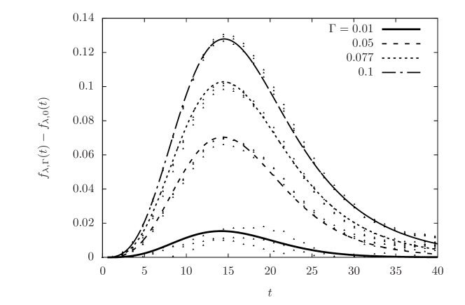
Figure 1: Generalized fidelity amplitude $f_{\lambda,\Gamma}(t)$ subtracted by $f_{\lambda}(t)$ for $\lambda=0.1$ and different values of $\Gamma$: $\Gamma=0.01$ (solid line), $0.05$ (dashed line), $0.077$ (dotted line), and $0.1$ (dashed-dotted line). The lines show the solutions of Eq.(25) and the points show the corresponding numerical simulations.

In Fig. 1 we can clearly see the influence of the coupling to the far environment, on the coherence measured in the central system. The effect scales with $\alpha=\Gamma/\lambda$, which, in this figure ranges from $\alpha=0.1$ to $\alpha=1$. Since the difference plotted is positive and increasing with $\alpha$, we confirm the effect discussed in Ref. [5], that increasing the coupling to the far environment, stabilizes the coherence in the central system. We also observe, that the theory obtained from Eq. (25) agrees very well with the numerical simulations for all values of $\alpha$ and for all times.

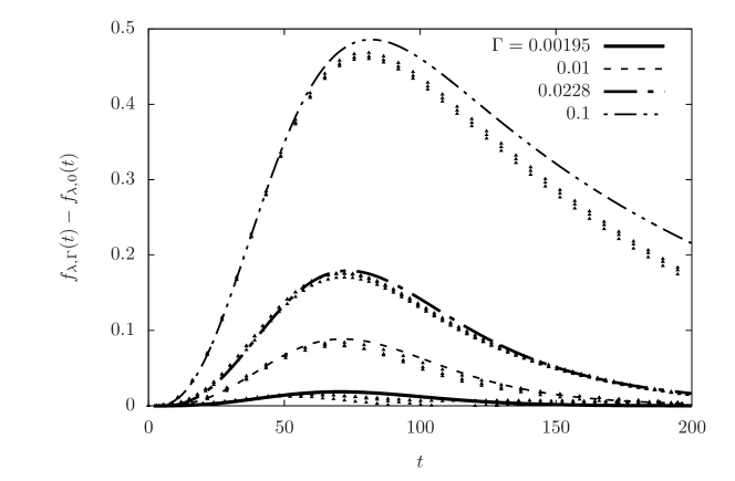
Figure 2: Generalized fidelity amplitude $f_{\lambda,\Gamma}(t)$ subtracted by $f_{\lambda}(t)$ for $\lambda=0.02$ and different values of $\Gamma$: $\Gamma=0.00195$ (solid line) $0.01$ (dashed line) $0.02285$ (dashed-dotted line) and $0.1$ (dashed-dashed-dotted-dotted line). The dashed lines show the solutions of Eq.(25) and the points show the corresponding numerical simulations.

In Fig. 2 we repeat the comparison but for the case of $\lambda=0.02$, which is well in the perturbative regime, where $f_{\lambda}(t)$ shows a Gaussian decay. Again we compare numerical simulations with the theoretical prediction from Eq. (25), for different values of $\alpha$. Here, these values range from $\alpha=0.0975$ up to $\alpha=5$. In this range, the stabilizing effect of the coupling to the far environment is even stronger. However, we also observe that the theoretical prediction systematically overestimates the effect, the larger $\alpha$ the larger the deviation. We suspect that these deviations might be a finite $N_{\rm e}$ effect.

4 Conclusions

We have presented a generalized fidelity amplitude, which starts out from the only direct measurement scheme for the fidelity amplitude [1], which uses a central system as a probe for the echo dynamics in the environment. We open the system to be probed to an additional outer environment and consider the decay of coherences of the probe. This we define to be proportional to the generalized fidelity amplitude. While this ensures that the quantity is measurable, it remains to be investigated how it relates to other generalizations of fidelity to open systems, such as the one by Josza [20].

We obtain a more general master equation, Eq. (17), which may be applied to integrable and non-integrable models for open quantum systems. The random matrix model considered here to illustrate our results, is slightly different from the model considered in [5], since there we considered the far environment to be a bath of harmonic oscillators described by the Caldeira-Leggett model of random Brownian motion [21]. Nevertheless, its effect on the near environment is equivalent and can be described by the same unique parameter $\Gamma$. We derived a new exact integral equation for the generalized fidelity amplitude, which constitutes significant progress comparing to previous work. Expanding this equation to lowest order in $\Gamma$ leads to the approximate analytical formula obtained in [5]. In Sec. 3, we find that its solution agrees with numerical simulations over a broad range of coupling strengths. This confirms the general experience, that increasing the coupling between near and far environment protects the coherence in the central system.

Acknowledgments

We thank C. Pineda and H.-J. Stöckmann for helpful discussions, and acknowledge the hospitality of the Centro Internacional de Ciencias, where these discussions took place. Finally, we acknowledge financial support from CONACyT through the grants CB-2009/129309 and 154586 as well as UNAM/DGAPA/PAPIIT IG 101113.

References

- [1] Gardiner SA, Cirac JI, Zoller P. 1997. Quantum chaos in an ion trap: the delta-kicked harmonic oscillator. Phys. Rev. Lett. 79, 4790–4793. doi:10.1103/PhysRevLett.79.4790.
- [2] Haug F, Bienert M, Schleich WP, Seligman TH, Raizen MG. 2005. Motional stability of the quantum kicked rotor: a fidelity approach. Phys. Rev. A 71, 043803. doi:10.1103/PhysRevA.71.043803.
- [3] Gorin T, Prosen T, Seligman TH, Strunz WT. 2004. Connection between decoherence and fidelity decay in echo dynamics. Phys. Rev. A 70, 042105. doi:10.1103/PhysRevA.70.042105.
- [4] Wu S, Tonyushkin A, Prentiss MG. 2009. Observation of saturation of fidelity decay with an atom interferometer. Phys. Rev. Lett. 103, 034101. doi:10.1103/PhysRevLett.103.034101.
- [5] Moreno HJ, Gorin T, Seligman TH. 2015. Improving coherence with nested environments. E-print arXiv:1502.04143v2.
- [6] Gorin T, Prosen T, Seligman TH, Žnidarič M. 2006. Dynamics of loschmidt echoes and fidelity decay. Phys. Rep. 435, 33–156. doi:10.1016/j.physrep.2006.09.003.
- [7] Gorini V, Kossakowski A, Sudarshan ECG. 1976. Completely positive dynamical semigroups of n-level systems. J. Math. Phy. 17, 821–825. doi:10.1063/1.522979.
- [8] Lindblad G. 1976. On the generators of quantum dynamical semigroups. Commun. Math. Phys. 48, 119. doi:10.1007/BF01608499.
- [9] Andersen MF, Kaplan A, Davidson N. 2003. Echo spectroscopy and quantum stability of trapped atoms. Phys. Rev. Lett. 90, 023001. doi:10.1103/PhysRevLett.90.023001.
- [10] Orear J, Fermi E. 1974. Nuclear Physics: A Course Given by Enrico Fermi at the University of Chicago. Chicago, USA: Midway reprint. University of Chicago Press.
- [11] Dirac PAM. 1927. The quantum theory of the emission and absorption of radiation. Proc. R. Soc. Lond. A, 114, 243–265. doi:10.1098/rspa.1927.0039.
- [12] Breuer H-P and Petruccione F. 2002. The Theory of Open Quantum Systems. Oxfort, UK: Oxford University Press.
- [13] Redfield AG. 1957. On the theory of relaxation processes IBM J. Res. Dev. 1, 19–31.
- [14] Gorin T, Pineda C, Kohler H, Seligman TH. 2008. A random matrix theory of decoherence. New J. Phys. 10, 115016. doi:10.1088/1367-2630/10/11/115016.
- [15] Pineda C, Gorin T, Seligman TH. 2007. Decoherence of two-qubit systems: a random matrix description. New J. Phys. 9, 106.
- [16] Kaplan L, Leyvraz F, Pineda C, Seligman TH. 2007. A trivial observation on time reversal in random matrix theory. J. Phys. A: Math. Theo. 40, F1063.
- [17] Arfken GB, Weber HJ. 2005. Mathematical methods for physicists, 6th Edition. Amsterdam, NL: Elsevier Academic Press.
- [18] Stöckmann H-J, Schäfer R. 2004. Recovery of the fidelity amplitude for the Gaussian ensembles. New J. Phys. 6, 199.
- [19] Gorin T, Prosen T, Seligman TH. 2004. A random matrix formulation of fidelity decay. New J. Phys. 6, 20.
- [20] Josza R. 1994. Fidelity for mixed quantum states. J. Mod. Opt. 41, 2315–2323.
- [21] Caldeira AO, Leggett AJ. 1983. Path integral approach to quantum brownian motion. Physica 121A, 587–616.