Gompertz - Power Series Distributions

Abstract

In this paper, we introduce the Gompertz power series (GPS) class of distributions which is obtained by compounding Gompertz and power series distributions. This distribution contains several lifetime models such as Gompertz-geometric (GG), Gompertz-Poisson (GP), Gompertz-binomial (GB), and Gompertz-logarithmic (GL) distributions as special cases. Sub-models of the GPS distribution are studied in details. The hazard rate function of the GPS distribution can be increasing, decreasing, and bathtub-shaped. We obtain several properties of the GPS distribution such as its probability density function, and failure rate function, Shannon entropy, mean residual life function, quantiles and moments. The maximum likelihood estimation procedure via a EM-algorithm is presented, and simulation studies are performed for evaluation of this estimation for complete data, and the MLE of parameters for censored data. At the end, a real example is given.

Keywords: EM algorithm; Gompertz distribution; Maximum likelihood estimation; Power series distributions.

1 Introduction

The exponential distribution is commonly used in many applied problems, particularly in lifetime data analysis. A generalization of this distribution is the Gompertz distribution. It is a lifetime distribution and is often applied to describe the distribution of adult life spans by actuaries and demographers. In some sciences such as biology, gerontology, computer, and marketing science, the Gompertz distribution is considered for the analysis of survival.

A random variable $X$ is said to have a Gompertz distribution, denoted by $X\sim G(\beta,\gamma)$, if its cumulative distribution function (cdf) is

$$G(x)=1-e^{-\frac{\beta}{\gamma}(e^{\gamma x}-1)},\;\;x\geq 0,\;\;\beta>0,\;\;\gamma>0,$$ (1.1)

and the probability density function (pdf) is

$$g(x)=\beta e^{\gamma x}e^{-\frac{\beta}{\gamma}(e^{\gamma x}-1)}.$$ (1.2)

The Gompertz distribution is a flexible distribution that can be skewed to the right and to the left. The hazard rate function of Gompertz distribution is $h_{g}(x)=\beta e^{\gamma x}$ which is a increasing function. The exponential distribution can be derived from the Gompertz distribution when $\gamma\rightarrow 0^{+}$.

Also, a discrete random variable, $N$ is a member of power series distributions (truncated at zero) if its probability mass function is given by

$$P(N=n)=\frac{a_{n}\theta^{n}}{C(\theta)},\;\;n=1,2,...,$$ (1.3)

where $a_{n}\geq 0$, $C(\theta)=\sum\limits_{n=1}^{\infty}a_{n}\theta^{n}$, and $\theta\in(0,s)$ is chosen such that $C(\theta)$ is finite and its first, second and third derivatives are defined and shown by $C^{\prime}(.)$, $C^{\prime\prime}(.)$ and $C^{\prime\prime\prime}(.)$. The term ”power series distribution” is generally credited to Noack (1950). This family of distributions includes many of the most common distributions, including the binomial, Poisson, geometric, negative binomial, logarithmic distributions. For more details of power series distributions, see Johnson et al. (2005), page 75.

In this paper, we compound the Gompertz and power series distributions and introduce a new class of distribution. This procedure follows similar way that was previously carried out by some authors: The exponential-power series distribution is introduced by Chahkandi and Ganjali (2009), which is included the exponential-geometric (Adamidis and Loukas, 1998; Adamidis et al., 2005), exponential-Poisson (Kuş, 2007), and exponential-logarithmic (Tahmasbi and Rezaei, 2008) distributions; the Weibull-power series distributions is introduced by Morais and Barreto-Souza (2011) which is a generalization of the exponential-power series distribution; the generalized exponential-power series distribution is introduced by Mahmoudi and Jafari (2012) which is included the Poisson-exponential (Cancho et al., 2011), complementary exponential-geometric (Louzada et al., 2011), and the complementary exponential-power series (Flores et al., 2011) distributions.

The remainder of our paper is organized as follows: in Section 2, we give the density and failure rate functions of the GPS distribution. Some properties such as quantiles, moments, order statistics, Shannon entropy and mean residual life are given in Section 3. Special cases of GPS distribution are given in Section 4. We discuss estimation by maximum likelihood and provide an expression for Fisher’s information matrix in Section 5. In this Section, we present the estimation based on EM-algorithm, and Section 6 contains Monte Carlo simulation results on the finite sample behavior of these estimators. In this Section, we also investigate the properties of MLE of parameters when the data are censored. An application of GPS distribution is given in the Section 7.

2 The Gompertz-power series model

The GPS model is derived as follows. Let $N$ be a random variable denoting the number of failure causes which it is a member of power series distributions (truncated at zero). For given $N$, let $X_{1},X_{2},...,X_{N}$ be independent identically distributed random variables from Gompertz distribution. If we consider $X_{(1)}=\min(X_{1},...,X_{N})$, then $X_{(1)}\mid N=n$ has Gompertz distribution with parameters $n\beta$ and $\gamma$. Therefore, the GPS class of distributions, denoted by $GPS(\beta,\gamma,\theta)$, is defined by

$$F(x)=1-\frac{C(\theta-\theta G(x))}{C(\theta)}=1-\frac{C(\theta e^{-\frac{\beta}{\gamma}(e^{\gamma x}-1)})}{C(\theta)},\ \ \ \ \ x>0.$$ (2.1)

The pdf of $GPS(\beta,\gamma,\theta)$ is given by

$$f(x)=\theta g(x)\frac{{C^{\prime}}(\theta-\theta G(x))}{C(\theta)}=\theta\beta e^{\gamma x}e^{-\frac{\beta}{\gamma}(e^{\gamma x}-1)}\frac{C^{\prime}(\theta e^{-\frac{\beta}{\gamma}(e^{\gamma x}-1)})}{C(\theta)}.$$ (2.2)

Proposition 1.

If $C(\theta)=\theta$, then the Gompertz distribution function concludes from the GPS distribution function in (2.1). Therefore, the Gompertz distribution is a special case of GPS distribution.

Proposition 2.

The limiting distribution of $GPS(\beta,\gamma,\theta)$ when $\theta\rightarrow 0^{+}$ is

$${\mathop{\lim}_{\theta\rightarrow 0^{+}}F(x)}=1-e^{\frac{-c\beta}{\gamma}(e^{\gamma x}-1)},$$

which is a $G(c\beta,\gamma)$, where $c=\min\{n\in N:a_{n}>0\}$.

Proposition 3.

The limiting distribution of $GPS(\beta,\gamma,\theta)$ when $\gamma\longrightarrow 0^{+}$ is

$${\mathop{\lim}_{\gamma\rightarrow 0^{+}}F(x)}=1-\frac{C(\theta e^{-\beta x})}{C(\theta)}.$$

In fact, it is the cdf of the exponential-power series (EPS) distribution and is introduced by Chahkandi and Ganjali (2009). This distribution contains several distributions; geometric-exponential distribution (Adamidis and Loukas, 1998; Adamidis et al., 2005), Poisson-exponential distribution (Kuş, 2007), and logarithmic-exponential distribution (Tahmasbi and Rezaei, 2008). Therefore, the GPS distribution is a generalization of EPS distribution. Note that EPS distribution is a distribution family with decreasing failure rate (hazard rate).

Proposition 4.

The densities of GPS class can be expressed as infinite linear combination of density of order distribution, i.e. it can be written as

$$f(x)=\sum\limits_{n=1}^{\infty}P(N=n)\ g_{(1)}(x;n),$$ (2.3)

where $g_{(1)}(x;n)$ is the pdf of $Y_{(1)}=\min(Y_{1},Y_{2},...,Y_{n})$, given by

$$g_{(1)}(x;n)=ng(x)[1-G(x)]^{n-1}=n\beta e^{\gamma x}e^{\frac{-n\beta}{\gamma}(e^{\gamma x}-1)},$$

i.e. Gompertz distribution with parameters $n\beta$ and $\gamma$.

Proposition 5.

The survival function and the hazard rate function of the GPS class of distributions, are given respectively by

$$S(x)=\frac{C(\theta e^{-\frac{\beta}{\gamma}(e^{\gamma x}-1)})}{C(\theta)},\ \ \ \ \ \ \ \ h(x)=\theta\beta e^{\gamma x}e^{-\frac{\beta}{\gamma}(e^{\gamma x}-1)}\frac{C^{\prime}(\theta e^{-\frac{\beta}{\gamma}(e^{\gamma x}-1)})}{C(\theta e^{-\frac{\beta}{\gamma}(e^{\gamma x}-1)})}.$$ (2.4)

Proposition 6.

For the pdf in (2.2) we have

$$\lim_{x\rightarrow 0^{+}}f(x)=\dfrac{\beta\theta C^{\prime}(\theta)}{C(\theta)}=\beta E(N),\ \ \ \ \lim_{x\rightarrow+\infty}f(x)=0.$$

Proposition 7.

For the hazard rate function, $h(x)$, in (2.4) we have

$$\lim_{x\rightarrow 0^{+}}h(x)=\lim_{x\rightarrow 0^{+}}f(x)=\dfrac{\beta\theta C^{\prime}(\theta)}{C(\theta)},\ \ \ \ \lim_{x\rightarrow+\infty}h(x)=+\infty.$$

Consider $C\left(\theta\right)=\theta+{\theta}^{20}$. Therefore, the pdf of GPS distribution is given as

$$f\left(x\right)=\beta e^{\gamma x}e^{-\frac{\beta}{\gamma}(e^{\gamma x}-1)}(1+20\theta^{19}e^{-\frac{19\beta}{\gamma}(e^{\gamma x}-1)})(1+{\theta}^{19})^{-1}.$$

The plots of this density and its hazard rate function, for some parameters are given in Figure 1. For $\beta=0.1,\gamma=3,\theta=1.0$, this density is bimodal, and the values of modes are 0.1582 and 1.1505.

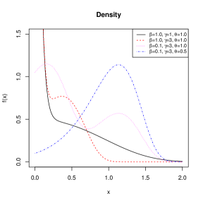
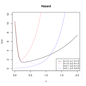
Figure 1: Plots of pdf and hazard rate functions of GPS with $C\left(\theta\right)=\theta+{\theta}^{20}$.

3 Statistical properties

In this section, some properties of the GPS distribution, such as quantiles, moments, order statistics, Shannon entropy and mean residual life are obtained.

3.1 Quantiles and Moments

The quantile $q$ of GPS distribution is given by

$$x_{q}=G^{-1}\left(1-\frac{1}{\theta}C^{-1}\left((1-q)C(\theta)\right)\right),\;\;\;\;\;0<q<1,$$

where $G^{-1}(y)=\frac{1}{\gamma}\log\left(1-\frac{\gamma}{\beta}\log(1-y)\right)$ and $C^{-1}(.)$ is the inverse function of $C(.)$. This result helps in simulating data from the GPS distribution with generating uniform distribution data.

For checking the consistency of the simulating data set form GPS distribution, the histogram for a generated data set with size 100 and the exact GPS density with $C\left(\theta\right)=\theta+{\theta}^{20}$, and parameters $\beta=0.1$, $\gamma=3$, $\theta=1.0$, are displayed in Figure 2 (left). Also, the empirical distribution function and the exact distribution function are given in Figure 2 (right).

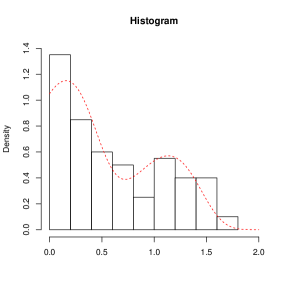
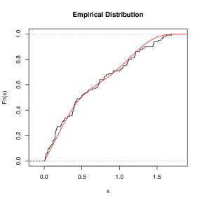
Figure 2: The histogram of a generated data set with size 100 and the exact GPS density (left) and the empirical distribution function and exact distribution function (right).

Now, we obtain the moment generating function of the GPS distribution by its Laplace transform. Consider $X\sim GPS(\beta,\gamma,\theta)$. Then, the Laplace transform of the GPS class can be expressed as

$$L(s)=E(e^{-sX})=\sum\limits_{n=1}^{\infty}P(N=n)L_{1}(s),$$ (3.1)

where

$$L_{1}(s)=\frac{n\beta}{\gamma}e^{\frac{n\beta}{\gamma}}W_{\frac{s}{\gamma}}(\frac{n\beta}{\gamma}),$$

is the Laplace transform of Gompertz distribution with parameters $n\beta$ and $\gamma$, and $W_{f}(z)=\int_{1}^{\infty}\frac{e^{-zu}}{u^{f}}du$. (see Lenart, 2012). Therefore, the moment generating function of the GPS distribution is

$$M_{X}(t)=\sum\limits_{n=1}^{\infty}P(N=n)L_{1}(-t)=\frac{\beta}{\gamma}\sum\limits_{n=1}^{\infty}\frac{a_{n}\theta^{n}}{C(\theta)}ne^{\frac{n\beta}{\gamma}}W_{\frac{-t}{\gamma}}(\frac{n\beta}{\gamma})=\frac{\beta}{\gamma}E[Ne^{\frac{N\beta}{\gamma}}W_{\frac{-t}{\gamma}}(\frac{N\beta}{\gamma})].$$ (3.2)

We can use $M_{X}(t)$ to obtain the central moment functions, $\mu_{r}=E[X^{r}]$. But from the direct calculation, we have

$$\mu_{r}=\int_{0}^{+\infty}x^{r}f(x)dx=\sum\limits_{n=1}^{\infty}P(N=n)E[Y_{(1)}^{r}],$$ (3.3)

where $E[Y_{(1)}^{r}]$ is the $r$th moment of $Y_{(1)}$, the Gompertz distribution with parameters $n\beta$ and $\gamma$, given by Lenart (2012) as

$$E[Y_{(1)}^{r}]=\frac{r!}{\gamma^{r}}e^{\frac{n\beta}{\gamma}}W_{1}^{r-1}(\frac{n\beta}{\gamma}),$$ (3.4)

where $W_{1}^{r-1}(z)=\frac{1}{(r-1)!}\int_{1}^{\infty}(\ln x)^{r-1}\frac{e^{-zx}}{x}dx$ is the generalised integro-exponential function. See Lenart (2012), for some expressions and approximations about the expected value and variance of Gompertz distribution. For example, when $\beta$ is close to $0$, an approximate result for $E[Y_{(1)}]$ is

$$E[Y_{(1)}]\approx\frac{1}{\gamma}e^{\frac{n\beta}{\gamma}}(\frac{n\beta}{\gamma}-\ln(\frac{n\beta}{\gamma})-0.57722).$$ (3.5)

3.2 Order statistic

Let $X_{1},X_{2},...,X_{n}$ be a random sample of size $n$ from $GPS(\beta,\gamma,\theta)$, then the pdf of the $i$th order statistic, say $X_{i:n}$, is given by

$$f_{i:n}(x)=\frac{n!}{(i-1)!(n-i)!}f(x)[1-\frac{C(\theta e^{-\frac{\beta}{\gamma}(e^{\gamma x}-1)})}{C(\theta)}]^{i-1}[\frac{C(\theta e^{-\frac{\beta}{\gamma}(e^{\gamma x}-1)})}{C(\theta)}]^{n-i},$$

where $f(.)$ is the pdf given by (2.2). Also, the cdf of $X_{i:n}$ is given by

$$F_{i:n}(x)=\frac{n!}{(i-1)!(n-i)!}\sum\limits_{k=0}^{n-i}\frac{(-1)^{k}\dbinom{n-i}{k}}{k+1}[1-\frac{C(\theta e^{-\frac{\beta}{\gamma}(e^{\gamma x}-1)})}{C(\theta)}]^{k+i},$$

An analytical expression for $r$th moment of order statistics $X_{i:n}$ is obtained as

$$E[X_{i:n}^{r}] = \sum\limits_{k=n-i+1}^{n}r(-1)^{k-n+i-1}\dbinom{k-1}{n-i}\dbinom{n}{k}\int_{0}^{+\infty}x^{r-1}S(x)^{k}dx$$ (3.6)

$$= \sum\limits_{k=n-i+1}^{n}\frac{r(-1)^{k-n+i-1}}{[C(\theta)]^{k}}\dbinom{k-1}{n-i}\dbinom{n}{k}\int_{0}^{+\infty}x^{r-1}[C(\theta e^{-\frac{\beta}{\gamma}(e^{\gamma x}-1)})]^{k}dx.$$

3.3 Shannon entropy and mean residual life

If $X$ is a none-negative continuous random variable with pdf $f(x)$, then Shannon’s entropy of $X$ is defined by Shannon (1948) as

$$H(f)=E[-\log f(X)]=-\int_{0}^{+\infty}f(x)\ln(f(x))dx,$$

and this is usually referred to as the continuous entropy (or differential entropy). An explicit expression of Shannon entropy for GPS distribution is obtained as

$$H(f)=-\log(\theta\beta)-\gamma\mu_{1}-\frac{\beta}{\gamma}+\frac{\beta}{\gamma}M_{X}(\gamma)+\log(C(\theta))-E_{N}[A(N,\theta)],$$ (3.7)

where $A(N,\theta)=\int_{0}^{1}Nu^{N-1}\log(C^{\prime}(\theta u))du$. Also, the mean residual life function of $X$ is given by

$$m(t)=E[X-t|X>t]=\frac{\int_{t}^{+\infty}(x-t)f(x)dx}{S(t)}=\frac{C(\theta)E_{N}[B(t,N,\beta,\gamma)]}{C(\theta e^{\frac{-\beta}{\gamma}(e^{\gamma x}-1)})}-t,$$

where $B(t,N,\beta,\gamma)=\int_{t}^{+\infty}N\beta xe^{\gamma x}e^{-\frac{N\beta}{\gamma}(e^{\gamma x}-1)}dx$.

4 Special cases of the GPS distributions

In this Section, we consider four special cases of the GPS distribution.

4.1 Gompertz - geometric distribution

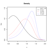
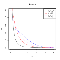
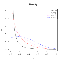
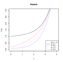
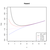
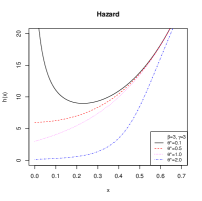
Figure 3: Plots of density and hazard rate functions of GG for different values $\beta$, $\gamma$ and $\theta^{*}$.

The geometric distribution (truncated at zero) is a special case of power series distributions with $a_{n}=1$ and $C(\theta)=\frac{\theta}{1-\theta}\ (0<\theta<1)$ . The pdf and hazard rate function of Gompertz-geometric (GG) distribution is given respectively by

$$f(x)=\frac{(1-\theta)\beta e^{\gamma x}e^{-\frac{\beta}{\gamma}(e^{\gamma x}-1)}}{(1-\theta e^{-\frac{\beta}{\gamma}(e^{\gamma x}-1)})^{2}},$$ (4.1)

and

$$h(x)=\frac{\beta e^{\gamma x}}{1-\theta e^{-\frac{\beta}{\gamma}(e^{\gamma x}-1)}}.$$ (4.2)

Remark 4.1.

When $\theta^{\ast}=1-\theta$, from (4.1) we have

$$f(x)=\frac{\theta^{*}\beta e^{\gamma x}e^{-\frac{\beta}{\gamma}(e^{\gamma x}-1)}}{(1-(1-\theta^{*})e^{-\frac{\beta}{\gamma}(e^{\gamma x}-1)})^{2}}.$$ (4.3)

Based on Marshall and Olkin (1997) $f(x)$ in (4.3) also is density for all $\theta^{*}>0$ ($\theta<1$).

Note that when $\gamma\rightarrow 0^{+}$, the pdf of extended exponential geometric (EEG) distribution (see Adamidis et al., 2005) concludes from the pdf in (4.3) with $\theta^{*}>0$. The EEG hazard function is monotonically increasing for $\theta^{*}>1$; decreasing for $0<\theta^{*}<1$ and constant for $\theta^{*}=1$.

Remark 4.2.

If $\theta^{*}=1$, then the pdf in (4.3) becomes the pdf of Gompertz distribution. Note that the hazard rate function of Gompertz distribution is increasing.

The plots of density and hazard rate function of GG distribution for different values of $\beta$, $\gamma$ and $\theta^{*}$ are given in Figure 3. We can see that the hazard rate function of GG distribution is increasing or bathtub.

4.2 Gompertz - Poisson distribution

The Poisson distribution (truncated at zero) is a special case of power series distributions with $a_{n}=\frac{1}{n!}$ and $C(\theta)=e^{\theta}-1\ (\theta>0).$ The pdf and hazard rate function of Gompertz-Poisson (GP) distribution are given respectively by

$$f(x)=\frac{\theta\beta e^{\gamma x}e^{-\frac{\beta}{\gamma}(e^{\gamma x}-1)}e^{\theta e^{-\frac{\beta}{\gamma}(e^{\gamma x}-1)}}}{e^{\theta}-1},$$ (4.4)

and

$$h(x)=\frac{\theta\beta e^{\gamma x}e^{-\frac{\beta}{\gamma}(e^{\gamma x}-1)}}{1-e^{-\theta e^{-\frac{\beta}{\gamma}(e^{\gamma x}-1)}}}.$$ (4.5)

The plots of density and hazard rate function of GP for different values of $\beta$, $\gamma$ and $\theta$ are given in Figure 4. We can see that the hazard rate function of GP distribution is increasing or bathtub.

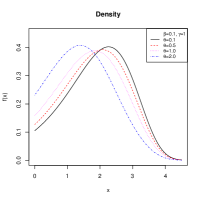
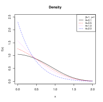
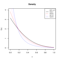
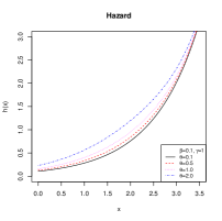
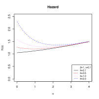
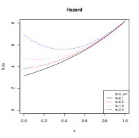
Figure 4: Plots of density and hazard rate functions of GP for different values $\beta$, $\gamma$ and $\theta$.

4.3 Gompertz - binomial distribution

The binomial distribution (truncated at zero) is a special case of power series distributions with $a_{n}=\dbinom{m}{n}$ and $C(\theta)=(\theta+1)^{m}-1\ (\theta>0),$ where $m$ $(n\leq m)$ is the number of replicas. The pdf and hazard rate function of Gompertz - binomial (GB) distribution are given respectively by

$$f(x)=\frac{m\theta\beta e^{\gamma x}e^{-\frac{\beta}{\gamma}(e^{\gamma x}-1)}(\theta e^{-\frac{\beta}{\gamma}(e^{\gamma x}-1)}+1)^{m-1}}{(\theta+1)^{m}-1},$$ (4.6)

and

$$h(x)=\frac{m\theta\beta e^{\gamma x}e^{-\frac{\beta}{\gamma}(e^{\gamma x}-1)}(\theta e^{-\frac{\beta}{\gamma}(e^{\gamma x}-1)}+1)^{m-1}}{(\theta e^{-\frac{\beta}{\gamma}(e^{\gamma x}-1)}+1)^{m}-1}.$$ (4.7)

The plots of density and hazard rate function of GB for $m=5$, and different values of $\beta$, $\gamma$ and $\theta$ are given in Figure 5. We can see that the hazard rate function of GB distribution is increasing or bathtub. We can find that the GP distribution can be obtained as limiting of GB distribution if $m\theta\longrightarrow\lambda>0$, when $m\longrightarrow\infty$.

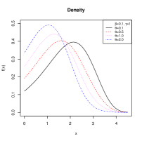
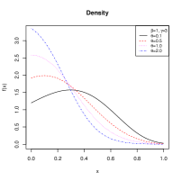
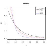
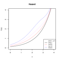
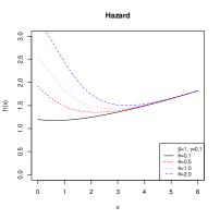
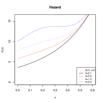
Figure 5: Plots of density and hazard rate functions of GB for $m=5$, and different values $\beta$, $\gamma$ and $\theta$.

4.4 Gompertz - logarithmic distribution

The logarithmic distribution (truncated at zero) is also a special case of power series distributions with $a_{n}=\frac{1}{n}$ and $C(\theta)=-\log(1-\theta)\ (0<\theta<1)$. The pdf and hazard rate function of Gompertz - logarithmic (GL) distribution are given respectively by

$$f(x)=\frac{\theta\beta e^{\gamma x}e^{-\frac{\beta}{\gamma}(e^{\gamma x}-1)}}{(\theta e^{-\frac{\beta}{\gamma}(e^{\gamma x}-1)}-1)\log(1-\theta)},$$ (4.8)

and

$$h(x)=\frac{\theta\beta e^{\gamma x}e^{-\frac{\beta}{\gamma}(e^{\gamma x}-1)}}{(\theta e^{-\frac{\beta}{\gamma}(e^{\gamma x}-1)}-1)\log(1-\theta e^{-\frac{\beta}{\gamma}(e^{\gamma x}-1)})}.$$ (4.9)

The plots of density and hazard rate function of GL for different values of $\beta$, $\gamma$ and $\theta$ are given in Figure 6. We can see that the hazard rate function of GL distribution is increasing or bathtub.

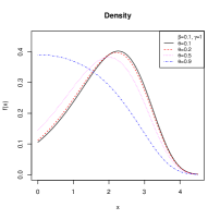
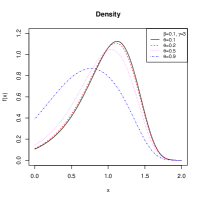
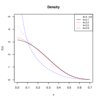
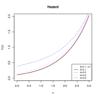
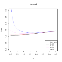
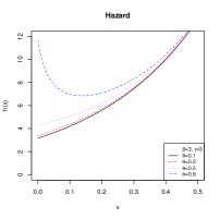
Figure 6: Plots of density and hazard rate functions of GL for different values $\beta$, $\gamma$ and $\theta$.

5 Estimation and inference

In this Section, we will derive the maximum likelihood estimators (MLE) of the unknown parameters ${\boldsymbol{\Theta}}=(\beta,\gamma,\theta)^{T}$ of the $GPS(\beta,\gamma,\theta)$. Also, asymptotic confidence intervals of these parameters will be derived based on the Fisher information. At the end, we will propose an Expectation - Maximization (EM) algorithm for estimating the parameters.

5.1 MLE for parameters

Let $X_{1},...,X_{n}$ be a random sample from $GPS(\beta,\gamma,\theta)$, and let ${\boldsymbol{x}}=(x_{1},...,x_{n})$ be the observed values of this random sample. The log-likelihood function is given by

$$l_{n}=l_{n}({\boldsymbol{\Theta}};{\boldsymbol{x}})=n\log(\theta)+n\log(\beta)+n\gamma\bar{x}+\sum\limits_{i=1}^{n}\log(t_{i})+\sum\limits_{i=1}^{n}\log(C^{\prime}(\theta t_{i}))-n\log(C(\theta)),$$

where $t_{i}=e^{-\frac{\beta}{\gamma}(e^{\gamma x_{i}}-1)}$. Therefore, the score function is given by $U({\boldsymbol{\Theta}};{\boldsymbol{x}})=(\frac{\partial l_{n}}{\partial\beta},\frac{\partial l_{n}}{\partial\gamma},\frac{\partial l_{n}}{\partial\theta})^{T}$, where

$$\frac{\partial l_{n}}{\partial\beta}=\frac{n}{\beta}+\frac{1}{\beta}\sum\limits_{i=1}^{n}\log(t_{i})+\frac{\theta}{\beta}\sum\limits_{i=1}^{n}\frac{t_{i}\log(t_{i})C^{\prime\prime}(\theta t_{i})}{C^{\prime}(\theta t_{i})},$$ (5.1)

$$\frac{\partial l_{n}}{\partial\gamma}=n\bar{x}+\sum\limits_{i=1}^{n}d_{i}+\theta\sum\limits_{i=1}^{n}\frac{b_{i}C^{\prime\prime}(\theta t_{i})}{C^{\prime}(\theta t_{i})},$$ (5.2)

$$\frac{\partial l_{n}}{\partial\theta}=\frac{n}{\theta}+\sum\limits_{i=1}^{n}\frac{t_{i}C^{\prime\prime}(\theta t_{i})}{C^{\prime}(\theta t_{i})}-\frac{nC^{\prime}(\theta)}{C(\theta)},$$ (5.3)

and $b_{i}=\frac{\partial t_{i}}{\partial\gamma}=t_{i}d_{i}$ and $d_{i}=\frac{\partial\log(t_{i})}{\partial\gamma}=\frac{1}{\gamma}(-\log(t_{i})+\gamma x_{i}\log(t_{i})-\beta x_{i})$.

The MLE of ${\boldsymbol{\Theta}}$, say $\hat{\boldsymbol{\Theta}}$, is obtained by solving the nonlinear system $U({\boldsymbol{\Theta}};{\boldsymbol{x}})={\boldsymbol{0}}$. We cannot get an explicit form for this nonlinear system of equations and they can be calculated by using a numerical method, like the Newton method or the bisection method.

For each element of the power series distributions (geometric, Poisson, logarithmic and binomial), we have the following theorems for the MLE’s:

Theorem 5.1.

Let ${\rm g_{1}}(\beta;\gamma,\theta,{\boldsymbol{x}})$ denote the function on RHS of the expression in (5.1), where $\gamma$ and $\theta$ are the true values of the parameters. Then, for a given $\gamma>0$, and $\theta>0$, the roots of ${\rm g}_{1}(\beta;\gamma,\theta,{\boldsymbol{x}})=0$, lies in the interval

$$\left(\frac{n}{\frac{\theta C^{\prime\prime}(\theta)}{C^{\prime}(\theta)}+1}{(-\sum^{n}_{i=1}\log(p_{i}))^{-1}}\ \ ,\ \ \ n{(-\sum^{n}_{i=1}\log(p_{i}))^{-1}}\right),$$

Proof.

See Appendix A.1. ∎

Theorem 5.2.

Let ${\rm g_{2}}(\gamma;\beta,\theta,x)$ denote the function on RHS of the expression in (5.2), where $\beta$ and $\theta$ are the true values of the parameters. Then, the equation ${\rm g_{2}}(\gamma;\beta,\theta,{\boldsymbol{x}})=0$ has at least one root if

$$n\bar{x}-\frac{\beta}{2}\sum^{n}_{i=1}{x^{2}_{i}(1+\frac{\theta e^{-\beta x_{i}}C^{\prime\prime}(\theta e^{-\beta x_{i}})}{C^{\prime}\left(\theta e^{-\beta x_{i}}\right)})}>0.$$

Proof.

See Appendix A.2. ∎

Theorem 5.3.

Let ${\rm g}_{3}(\theta;\beta,\gamma,{\boldsymbol{x}})$ denote the function on RHS of the expression in (5.3), where $\beta$ and $\gamma$ are the true values of the parameters.
a. The equation ${\rm g}_{3}(\theta;\beta,\gamma,{\boldsymbol{x}})=0$ has at least one root if for all GG, GP and GL distributions $\sum\limits_{i=1}^{n}t_{i}>\frac{n}{2}$.
b. If ${\rm g}_{3}(p;\beta,\gamma,{\boldsymbol{x}})=\frac{\partial l_{n}}{\partial p}$, where $p=\frac{\theta}{\theta+1}$ and $p\in(0,1)$ then the equation ${\rm g}_{3}(\theta;\beta,\gamma,{\boldsymbol{x}})=0$ has at least one root for GB distribution if $\sum\limits_{i=1}^{n}t_{i}>\frac{n}{2}$ and $\sum\limits_{i=1}^{n}\frac{1}{t_{i}}>\frac{nm}{1-m}$.

Proof.

See Appendix A.3. ∎

Theorem 5.4.

The pdf, $f(x|{\boldsymbol{\Theta}})$, of GPS distribution satisfies on the regularity condistions, i.e.

• the support of $f(x|{\boldsymbol{\Theta}})$ does not depend on ${\boldsymbol{\Theta}}$,

• $f(x|{\boldsymbol{\Theta}})$ is twice continuously differentiable with respect to ${\boldsymbol{\Theta}}$,

• the differentiation and integration are interchangeable in the sense that

$$\frac{\partial}{\partial{\boldsymbol{\Theta}}}\int_{-\infty}^{\infty}f(x|{\boldsymbol{\Theta}})dx=\int_{-\infty}^{\infty}\frac{\partial}{\partial{\boldsymbol{\Theta}}}f(x|{\boldsymbol{\Theta}})dx,\ \ \ \ \ \ \frac{\partial^{2}}{\partial{\boldsymbol{\Theta}}\partial{\boldsymbol{\Theta}}^{T}}\int_{-\infty}^{\infty}f(x|{\boldsymbol{\Theta}})dx=\int_{-\infty}^{\infty}\frac{\partial^{2}}{\partial{\boldsymbol{\Theta}}\partial{\boldsymbol{\Theta}}^{T}}f(x|{\boldsymbol{\Theta}})dx.$$

Proof.

The proof is obvious and for more details, see Casella and Berger (2001) Section 10. ∎

Now, we derive asymptotic confidence intervals for the parameters of GPS distribution. It is well-known that under regularity conditions (see Casella and Berger, 2001, Section 10), the asymptotic distribution of $\sqrt{n}(\hat{\boldsymbol{\Theta}}-{\boldsymbol{\Theta}})$ is multivariate normal with mean ${\boldsymbol{0}}$ and variance-covariance matrix $J_{n}^{-1}({\boldsymbol{\Theta}})$, where $J_{n}({\boldsymbol{\Theta}})=\lim_{n\rightarrow 0}I_{n}({\boldsymbol{\Theta}})$, and $I_{n}({\boldsymbol{\Theta}})$ is the $3\times 3$ observed information matrix, i.e.

$$I_{n}\left({\boldsymbol{\Theta}}\right)=-\left[\begin{array}[]{ccc}I_{\beta\beta}&I_{\beta\gamma}&I_{\beta\theta}\\ I_{\beta\gamma}&I_{\gamma\gamma}&I_{\gamma\theta}\\ I_{\beta\theta}&I_{\gamma\theta}&I_{\theta\theta}\end{array}\right],$$

whose elements are given in Appendix B. Therefore, an $100(1-\alpha)$ asymptotic confidence interval for each parameter, ${\boldsymbol{\Theta}}_{r}$, is given by

$$ACI_{r}=(\hat{\boldsymbol{\Theta}}_{r}-Z_{\alpha/2}\sqrt{\hat{I}_{rr}},\hat{\boldsymbol{\Theta}}_{r}+Z_{\frac{\alpha}{2}}\sqrt{\hat{I}_{rr}}),$$ (5.4)

where $\hat{I}_{rr}$ is the $(r,r)$ diagonal element of $I_{n}^{-1}(\hat{\boldsymbol{\Theta}})$ for $r=1,2,3$ and $Z_{\alpha/2}$ is the quantile $\frac{\alpha}{2}$ of the standard normal distribution.

In some cases, a censoring time $C_{i}$ is assumed in collecting the lifetime data $X_{i}$, where $C_{i}$ and $X_{i}$ are independent. Suppose that the data consist of $n$ independent observations $x_{i}=\min(X_{i},C_{i})$ and $\delta_{i}=I(X_{i}\leq C_{i})$ is such that $\delta_{i}=1$ if $X_{i}$ is a time to event and $\delta_{i}=0$ if it is right censored for $i=1,\dots,n$. The censored likelihood function is

$$L_{S}({\boldsymbol{\Theta}})\varpropto\prod_{i=1}^{n}[f(x_{i}|{\boldsymbol{\Theta}})]^{\delta_{i}}[S(x_{i}|{\boldsymbol{\Theta}})]^{1-\delta_{i}},$$ (5.5)

where $f(x_{i}|{\boldsymbol{\Theta}})$ and $S(x_{i}|{\boldsymbol{\Theta}})$ are the density function and survival function of GPS distribution. A similar procedure to the above can be used for constructing confidence interval for the parameters of the GPS model with a censoring time.

5.2 EM-algorithm

The EM algorithm is a very powerful tool in handling the incomplete data problem (see Dempster et al., 1977). It is an iterative method, and there are two steps in each iteration: Expectation step or the E-step and the Maximization step or the M-step. The EM algorithm is especially useful if the complete data set is easy to analyze. In this Section, we develop an EM-algorithm for obtaining the MLE’s for the parameters of GPS distribution.

We define a hypothetical complete-data distribution with a joint probability density function in the form

$$g(x_{i},z_{i};{\boldsymbol{\Theta}})=z_{i}\beta e^{\gamma x_{i}}e^{-\frac{z_{i}\beta}{\gamma}(e^{\gamma x_{i}}-1)}\frac{a_{z_{i}}\theta^{z_{i}}}{C(\theta)},$$

where $\beta$, $\gamma$, $\theta>0$, $x_{i}>0$ and $z_{i}\in N$. Therefore, the log-likelihood for the complete-data is

$$l^{\ast}({\boldsymbol{y}};{\boldsymbol{\Theta}})\propto n\bar{z}\log(\theta)+n\log(\beta)+n\gamma\bar{x}-\frac{\beta}{\gamma}\sum\limits_{i=1}^{n}z_{i}(e^{\gamma x_{i}}-1)-n\log(C(\theta)),$$ (5.6)

where ${\boldsymbol{y}}=(x_{1},...,x_{n},z_{1},...,z_{n})$, $\bar{z}=n^{-1}\sum\limits_{i=1}^{n}z_{i}$, and $\bar{x}=n^{-1}\sum\limits_{i=1}^{n}x_{i}$. On differentiation (5.6) with respect to parameters $\beta$, $\gamma$, and $\theta$, we obtain the components of the score function, $U({\boldsymbol{y}};{\boldsymbol{\Theta}})=(\frac{\partial l^{\ast}_{n}}{\partial\beta},\frac{\partial l^{\ast}_{n}}{\partial\gamma},\frac{\partial l^{\ast}_{n}}{\partial\theta})^{\prime}$, as

$$\frac{\partial l^{\ast}_{n}}{\partial\beta} = \frac{n}{\beta}-\frac{1}{\gamma}\sum\limits_{i=1}^{n}z_{i}(e^{\gamma x_{i}}-1),$$

$$\frac{\partial l^{\ast}_{n}}{\partial\gamma} = n\bar{x}+\frac{\beta}{\gamma^{2}}\sum\limits_{i=1}^{n}z_{i}(e^{\gamma x_{i}}-1)-\frac{\beta}{\gamma}\sum\limits_{i=1}^{n}z_{i}x_{i}e^{\gamma x_{i}},$$

$$\frac{\partial l^{\ast}_{n}}{\partial\theta} = \frac{n\bar{z}}{\theta}-n\frac{C^{\prime}(\theta)}{C(\theta)}.$$

From a nonlinear system of equations $U({\boldsymbol{y}};{\boldsymbol{\Theta}})={\boldsymbol{0}}$, we obtain the iterative procedure of the EM-algorithm as

$$\hat{\beta}^{(t+1)}=\frac{n\gamma^{(t)}}{\sum\limits_{i=1}^{n}\hat{z}_{i}^{(t)}(e^{\hat{\gamma}^{(t)}x_{i}}-1)},\qquad\hat{\theta}^{(t+1)}=\frac{C(\hat{\theta}^{(t+1)})}{nC^{\prime}(\hat{\theta}^{(t+1)})}\sum\limits_{i=1}^{n}\hat{z}_{i}^{(t)},$$

$$n\bar{x}(\hat{\gamma}^{(t+1)})^{2}+\hat{\beta}^{(t)}\sum\limits_{i=1}^{n}\hat{z}^{(t)}_{i}(e^{\hat{\gamma}^{(t+1)}x_{i}}-1)-\hat{\gamma}^{(t+1)}\hat{\beta}^{(t)}\sum\limits_{i=1}^{n}{\hat{z}}^{(t)}_{i}x_{i}e^{\hat{\gamma}^{(t+1)}x_{i}}=0,$$

where $\hat{\theta}^{(t+1)}$ and $\hat{\gamma}^{(t+1)}$ are found numerically. Here, for $i=1,2,...,n$, we have that

$$\hat{z}_{i}^{(t)}=1+\frac{\hat{\theta}^{(t)}e^{-\frac{\hat{\beta}^{(t)}}{\hat{\gamma}^{(t)}}(e^{\hat{\gamma}^{(t)}x_{i}}-1)}C^{\prime\prime}(\hat{\theta}^{(t)}e^{-\frac{\hat{\beta}^{(t)}}{\hat{\gamma}^{(t)}}(e^{\hat{\gamma}^{(t)}x_{i}}-1)})}{C^{\prime}(\hat{\theta}^{(t)}e^{-\frac{\hat{\beta}^{(t)}}{\hat{\gamma}^{(t)}}(e^{\hat{\gamma}^{(t)}x_{i}}-1)})}.$$

In this part, we use the results of Louis (1982) to obtain the standard errors of the estimators from the EM-algorithm. The elements of the $3\times 3$ observed information matrix $I_{c}({\boldsymbol{\Theta}};{\boldsymbol{y}})=-[\frac{\partial U({\boldsymbol{y}};{\boldsymbol{\Theta}})}{\partial{\boldsymbol{\Theta}}}]$ are given by

$$-\frac{\partial^{2}l^{\ast}_{n}}{\partial\beta^{2}}=\frac{n}{\beta^{2}},\quad-\frac{\partial^{2}l^{\ast}_{n}}{\partial\beta\partial\gamma}=-\frac{\partial^{2}l^{\ast}_{n}}{\partial\gamma\partial\beta}=-\frac{1}{\gamma^{2}}\sum\limits_{i=1}^{n}z_{i}(e^{\gamma x_{i}}-1)+\frac{1}{\gamma}\sum\limits_{i=1}^{n}z_{i}x_{i}e^{\gamma x_{i}},$$

$$\ \frac{\partial^{2}l^{\ast}_{n}}{\partial\beta\partial\theta}=\frac{\partial^{2}l^{\ast}_{n}}{\partial\theta\partial\beta}=\frac{\partial^{2}l^{\ast}_{n}}{\partial\theta\partial\gamma}=\frac{\partial^{2}l^{\ast}_{n}}{\partial\gamma\partial\theta}=0,\quad-\frac{\partial^{2}l^{\ast}_{n}}{\partial\theta^{2}}=\frac{n\bar{z}}{\theta^{2}}+\frac{nC^{\prime\prime}(\theta)}{C(\theta)}-\frac{n(C^{\prime}(\theta))^{2}}{(C(\theta))^{2}},$$

$$-\frac{\partial^{2}l^{\ast}_{n}}{\partial\gamma^{2}}=\frac{2\beta}{\gamma^{3}}\sum\limits_{i=1}^{n}z_{i}(e^{\gamma x_{i}}-1)-\frac{2\beta}{\gamma^{2}}\sum\limits_{i=1}^{n}z_{i}x_{i}e^{\gamma x_{i}}+\frac{\beta}{\gamma}\sum\limits_{i=1}^{n}z_{i}x_{i}^{2}e^{\gamma x_{i}}.$$

Taking the conditional expectation of $I_{c}({\boldsymbol{\Theta}};{\boldsymbol{y}})$ given ${\boldsymbol{x}}$, we obtain the $3\times 3$ matrix

$${\mathcal{I}}_{c}({\boldsymbol{\Theta}};{\boldsymbol{x}})=E(I_{c}({\boldsymbol{\Theta}};{\boldsymbol{y}})|{\boldsymbol{x}})=[c_{ij}],$$

where

$$c_{11}=\frac{n}{\beta^{2}},\quad c_{12}=c_{21}=-\frac{1}{\gamma^{2}}\sum\limits_{i=1}^{n}E(Z_{i}|x_{i})(e^{\gamma x_{i}}-1)+\frac{1}{\gamma}\sum\limits_{i=1}^{n}E(Z_{i}|x_{i})x_{i}e^{\gamma x_{i}},$$

$$c_{13}=c_{31}=c_{23}=c_{32}=0,\quad c_{33}=\frac{1}{\theta^{2}}\sum\limits_{i=1}^{n}E(Z_{i}|x_{i})+\frac{nC^{\prime\prime}(\theta)}{C(\theta)}-\frac{n(C^{\prime}(\theta))^{2}}{(C(\theta))^{2}},$$

$$c_{22}=\frac{2\beta}{\gamma^{3}}\sum\limits_{i=1}^{n}E(Z_{i}|x_{i})(e^{\gamma x_{i}}-1)-\frac{2\beta}{\gamma^{2}}\sum\limits_{i=1}^{n}E(Z_{i}|x_{i})x_{i}e^{\gamma x_{i}}+\frac{\beta}{\gamma}\sum\limits_{i=1}^{n}E(Z_{i}|x_{i})x_{i}^{2}e^{\gamma x_{i}},$$

and

$$E(Z_{i}|x_{i})=1+\frac{\theta e^{-\frac{\beta}{\gamma}(e^{\gamma x_{i}}-1)}C^{\prime\prime}(\theta e^{-\frac{\beta}{\gamma}(e^{\gamma x_{i}}-1)})}{C^{\prime}(\theta e^{-\frac{\beta}{\gamma}(e^{\gamma x_{i}}-1)})}.$$

Moving now to the computation of ${\mathcal{I}}_{m}(\Theta;\boldsymbol{x})$ as

$${\mathcal{I}}_{m}({\boldsymbol{\Theta}};{\boldsymbol{x}})=Var[U({\boldsymbol{y}};{\boldsymbol{\Theta}})|{\boldsymbol{x}}]=[v_{ij}],$$

where

$$v_{11}=\frac{1}{\gamma^{2}}\sum\limits_{i=1}^{n}(e^{\gamma x_{i}}-1)^{2}Var(Z_{i}|x_{i}),\quad v_{13}=v_{31}=-\frac{1}{\gamma\theta}\sum\limits_{i=1}^{n}(e^{\gamma x_{i}}-1)Var(Z_{i}|x_{i}),$$

$$v_{12}=v_{21}=-\frac{\beta}{\gamma^{3}}\sum\limits_{i=1}^{n}(e^{\gamma x_{i}}-1)(e^{\gamma x_{i}}-1-\gamma x_{i}e^{\gamma x_{i}})Var(Z_{i}|x),$$

$$v_{22}=\frac{\beta^{2}}{\gamma^{4}}\sum\limits_{i=1}^{n}(e^{\gamma x_{i}}-1-\gamma x_{i}e^{\gamma x_{i}})^{2}Var(Z_{i}|x_{i}),$$

$$v_{23}=v_{32}=\frac{\beta}{\theta\gamma^{2}}\sum\limits_{i=1}^{n}(e^{\gamma x_{i}}-1-\gamma x_{i}e^{\gamma x_{i}})Var(Z_{i}|x_{i}),\quad v_{33}=\frac{1}{\theta^{2}}\sum\limits_{i=1}^{n}Var(Z_{i}|x_{i}),$$

and

$$Var(Z|x) = E(Z^{2}|x)-(E(Z|x))^{2}$$

$$= \frac{1}{C^{\prime}(\theta_{\ast})}\sum\limits_{z=1}^{\infty}a_{z}z^{3}\theta_{\ast}^{z-1}-\frac{1}{[C^{\prime}(\theta_{\ast})]^{2}}[C^{\prime}(\theta_{\ast})+\theta_{\ast}C^{\prime\prime}(\theta_{\ast})]^{2}$$

$$= \frac{1}{C^{\prime}(\theta_{\ast})}[\theta_{\ast}^{2}C^{\prime\prime\prime}(\theta_{\ast})+C^{\prime}(\theta_{\ast})+3\theta_{\ast}C^{\prime\prime}(\theta_{\ast})]-\frac{1}{[C^{\prime}(\theta_{\ast})]^{2}}[C^{\prime}(\theta_{\ast})+\theta_{\ast}C^{\prime\prime}(\theta_{\ast})]^{2},$$

in which $\theta_{\ast}=\theta e^{-\frac{\beta}{\gamma}(e^{\gamma x}-1)}$. Therefore, we obtain the observed information as

$$I(\hat{{\boldsymbol{\Theta}}};{\boldsymbol{x}})=\mathcal{I}_{c}(\hat{\boldsymbol{\Theta}};{\boldsymbol{x}})-\mathcal{I}_{m}(\hat{\boldsymbol{\Theta}};{\boldsymbol{x}}).$$

The standard errors of the MLE’s of the EM-algorithm are the square root of the diagonal elements of the $I^{-1}(\hat{\boldsymbol{\Theta}};{\boldsymbol{x}})$.

6 Simulation

This section presents the results of three simulation studies. First, a simulation study is performed for evaluation of parameter estimation based on the EM algorithm. No restriction has been imposed on the maximum number of iterations and convergence is assumed when the absolute difference between successive estimates are less that $10^{-4}$.

Here, we consider the GG distribution and generate $N=1000$ random samples with different set of parameters for $n=30,50,100,200$. In each random sample, the estimation of parameters as well as the Fisher information matrix are obtained. Then, the average value of estimations (AE), mean square errors (MSE), variance of estimations (VS), the average value of inverse of Fisher information (EF) matrices, and coverage probabilities (CP) of the 95% confidence interval in (5.4) are computed. The results are given in Table 1, and we can conclude that

Table 1: The average MLE’s, mean square errors, variance of estimations, the average value of Fisher information, and coverage probability based on EM estimators for GG distribution

	Parameter			AE			MSE			VS			EF			CP
$n$	$\beta$	$\gamma$	$\theta$	$\hat{\beta}$	$\hat{\gamma}$	$\hat{\theta}$	$\hat{\beta}$	$\hat{\gamma}$	$\hat{\theta}$	$\hat{\beta}$	$\hat{\gamma}$	$\hat{\theta}$	$\hat{\beta}$	$\hat{\gamma}$	$\hat{\theta}$	${\beta}$	${\gamma}$	${\theta}$
30	0.5	2.0	0.9	0.490	2.760	0.891	0.914	4.601	0.466	0.102	1.553	0.008	1.748	6.111	0.089	0.90	0.94	0.91
50	0.5	2.0	0.9	0.458	2.582	0.903	0.939	3.538	0.460	0.092	1.084	0.005	1.593	4.836	0.076	0.92	0.94	0.91
100	0.5	2.0	0.9	0.446	2.451	0.908	1.004	2.796	0.461	0.108	0.666	0.005	0.882	2.723	0.041	0.95	0.95	0.95
200	0.5	2.0	0.9	0.470	2.283	0.904	0.941	2.170	0.454	0.112	0.442	0.005	0.679	1.716	0.027	0.95	0.95	0.96
30	0.5	2.0	0.1	0.406	2.711	0.207	1.020	4.774	0.994	0.039	0.745	0.107	1.774	5.318	5.722	0.89	0.96	0.87
50	0.5	2.0	0.1	0.427	2.587	0.187	1.004	4.149	1.004	0.039	0.531	0.102	1.143	3.119	3.222	0.90	0.94	0.88
100	0.5	2.0	0.1	0.457	2.418	0.131	0.951	3.371	1.030	0.032	0.311	0.086	1.790	5.490	6.589	0.92	0.96	0.90
200	0.5	2.0	0.1	0.485	2.300	0.192	0.914	2.948	1.036	0.027	0.211	0.076	0.835	2.103	2.602	0.92	0.95	0.92
30	1.0	2.0	0.9	0.859	3.441	0.915	0.764	8.083	0.401	0.213	3.115	0.005	4.490	14.220	0.060	0.91	0.93	0.93
50	1.0	2.0	0.9	0.911	3.123	0.913	0.924	5.636	0.399	0.466	2.097	0.006	4.339	9.036	0.051	0.91	0.94	0.92
100	1.0	2.0	0.9	0.913	2.684	0.903	1.223	3.474	0.417	0.854	1.385	0.011	3.445	5.108	0.042	0.92	0.96	0.92
200	1.0	2.0	0.9	1.033	2.378	0.893	1.234	2.369	0.420	0.964	1.024	0.011	2.393	3.437	0.027	0.92	0.95	0.93
30	1.0	2.0	0.1	0.261	2.972	0.274	0.962	5.359	1.006	0.128	0.998	0.088	6.823	10.343	6.991	0.89	0.93	0.91
50	1.0	2.0	0.1	0.214	2.814	0.228	0.912	4.528	1.057	0.133	0.759	0.089	4.393	5.565	3.258	0.89	0.92	0.91
100	1.0	2.0	0.1	0.185	2.556	0.179	0.824	3.360	1.103	0.125	0.462	0.083	2.599	3.426	2.167	0.91	0.94	0.93
200	1.0	2.0	0.1	0.155	2.411	0.117	0.771	2.829	1.173	0.107	0.336	0.076	1.841	2.406	1.618	0.92	0.93	0.93

Table 2: The average MLE’s, mean square errors, variance of estimations, the average value of Fisher information, and coverage probability based on MLE estimators for GG distribution with censored data

	Parameter			AE			MSE			VS			EF			CP
$n$	$\beta$	$\gamma$	$\theta$	$\hat{\beta}$	$\hat{\gamma}$	$\hat{\theta}$	$\hat{\beta}$	$\hat{\gamma}$	$\hat{\theta}$	$\hat{\beta}$	$\hat{\gamma}$	$\hat{\theta}$	$\hat{\beta}$	$\hat{\gamma}$	$\hat{\theta}$	${\beta}$	${\gamma}$	${\theta}$
30	0.5	2.0	0.9	1.141	2.536	0.705	1.613	2.092	0.132	1.203	1.807	0.094	16.115	14.718	5.692	0.86	0.93	0.84
50	0.5	2.0	0.9	0.898	2.300	0.778	0.866	1.431	0.071	0.709	1.342	0.056	8.758	6.669	2.715	0.88	0.94	0.87
100	0.5	2.0	0.9	0.789	2.062	0.822	0.651	0.862	0.040	0.568	0.859	0.034	7.289	5.956	2.069	0.88	0.95	0.88
200	0.5	2.0	0.9	0.670	2.042	0.856	0.326	0.633	0.018	0.297	0.632	0.016	4.143	5.705	1.008	0.91	0.95	0.90
30	0.5	2.0	0.1	0.399	2.367	0.232	0.059	0.568	0.138	0.049	0.434	0.121	4.323	8.031	6.697	0.91	0.92	0.90
50	0.5	2.0	0.1	0.389	2.343	0.260	0.061	0.485	0.154	0.049	0.368	0.128	3.002	6.738	4.966	0.91	0.92	0.91
100	0.5	2.0	0.1	0.386	2.304	0.293	0.066	0.422	0.174	0.053	0.330	0.137	3.390	4.996	4.715	0.89	0.93	0.89
200	0.5	2.0	0.1	0.377	2.316	0.307	0.063	0.363	0.179	0.048	0.263	0.136	1.195	4.790	3.744	0.89	0.95	0.90
30	1.0	2.0	0.9	1.995	2.849	0.746	4.086	3.014	0.091	3.098	2.294	0.068	16.988	18.095	3.081	0.87	0.90	0.85
50	1.0	2.0	0.9	1.667	2.594	0.799	2.727	2.201	0.052	2.284	1.851	0.042	15.772	17.097	2.365	0.86	0.91	0.84
100	1.0	2.0	0.9	1.308	2.208	0.851	1.428	1.120	0.025	1.335	1.078	0.022	13.458	15.288	1.799	0.85	0.94	0.82
200	1.0	2.0	0.9	1.191	2.064	0.871	0.902	0.552	0.013	0.866	0.548	0.012	10.675	9.313	1.069	0.88	0.93	0.87
30	1.0	2.0	0.1	0.616	2.994	0.367	0.296	2.448	0.215	0.149	1.460	0.144	8.004	9.443	6.819	0.84	0.93	0.84
50	1.0	2.0	0.1	0.628	2.882	0.389	0.308	2.110	0.232	0.170	1.333	0.148	6.905	4.961	5.584	0.80	0.95	0.81
100	1.0	2.0	0.1	0.630	2.816	0.407	0.325	1.762	0.253	0.188	1.098	0.159	5.158	4.707	4.130	0.74	0.89	0.75
200	1.0	2.0	0.1	0.631	2.723	0.413	0.326	1.331	0.260	0.190	0.809	0.162	5.089	3.507	3.174	0.73	0.91	0.74

Table 3: The number of cases that the criteria value of fitted distribution is smaller than the criteria value of fitted GG distribution

	Parameter			AIC				AICC				BIC
$n$	$\beta$	$\gamma$	$\theta$	Gompertz	GP	GB	GL	Gompertz	GP	GB	GL	Gompertz	GP	GB	GL
30	0.5	2.0	0.9	761	81	71	457	821	81	71	457	902	81	71	457
50	0.5	2.0	0.9	648	95	84	419	703	95	84	419	901	95	84	419
100	0.5	2.0	0.9	360	60	48	375	387	60	48	375	776	60	48	375
200	0.5	2.0	0.9	146	39	30	363	152	39	30	363	541	39	30	363
30	0.5	2.0	0.1	945	18	24	350	959	18	24	350	978	18	24	350
50	0.5	2.0	0.1	933	19	41	386	946	19	41	386	986	19	41	386
100	0.5	2.0	0.1	917	23	52	418	924	23	52	418	990	23	52	418
200	0.5	2.0	0.1	894	33	73	408	899	33	73	408	988	33	73	408
30	1.0	2.0	0.9	492	123	102	460	588	123	102	460	706	123	102	460
50	1.0	2.0	0.9	279	139	120	397	308	139	120	397	539	139	120	397
100	1.0	2.0	0.9	84	112	82	363	89	112	82	363	282	112	82	363
200	1.0	2.0	0.9	12	61	43	328	15	61	43	328	80	61	43	328
30	1.0	2.0	0.1	965	25	28	333	973	25	28	333	984	25	28	333
50	1.0	2.0	0.1	954	16	32	352	965	16	32	352	997	16	32	352
100	1.0	2.0	0.1	954	25	64	364	958	25	64	364	992	25	64	364
200	1.0	2.0	0.1	921	36	64	387	927	36	64	387	994	36	64	387

Table 4: The number of cases that the criteria value of fitted distribution is smaller than the criteria value of fitted Gompertz distribution

	Parameter			AIC				AICC				BIC
$n$	$\beta$	$\gamma$	$\theta$	GG	GP	GB	GL	GG	GP	GB	GL	GG	GP	GB	GL
30	0.5	2.0	0.9	54	13	6	231	34	7	5	180	16	5	1	92
50	0.5	2.0	0.9	71	39	21	173	58	25	14	156	20	3	1	68
100	0.5	2.0	0.9	59	39	34	161	53	37	32	150	12	3	4	47
200	0.5	2.0	0.9	68	68	69	145	65	64	62	141	4	3	1	25
30	0.5	2.0	0.1	47	8	1	108	28	3	0	81	12	0	0	44
50	0.5	2.0	0.1	57	6	3	122	49	5	1	110	13	0	0	42
100	0.5	2.0	0.1	97	13	21	116	86	10	15	115	13	0	1	25
200	0.5	2.0	0.1	129	35	31	95	122	35	30	95	17	1	0	20
30	1.0	2.0	0.9	52	7	3	48	39	0	0	43	18	0	0	29
50	1.0	2.0	0.9	53	20	10	37	44	10	5	34	13	0	0	17
100	1.0	2.0	0.9	74	30	40	25	68	24	32	24	10	1	0	8
200	1.0	2.0	0.9	76	42	55	7	71	37	52	7	5	2	1	3
30	1.0	2.0	0.1	34	0	1	93	20	0	0	79	5	0	0	51
50	1.0	2.0	0.1	47	3	0	88	42	2	0	73	15	0	0	26
100	1.0	2.0	0.1	65	0	1	100	61	0	1	89	8	0	0	21
200	1.0	2.0	0.1	86	4	4	91	80	4	4	86	13	0	0	8

i) convergence has been achieved in all cases and this emphasizes the numerical stability of the EM-algorithm, ii) the differences between the average estimates and the true values are almost small, iii) the MSE, variance of estimations, and variance based on Fisher information matrices decrease when the sample size increases, iv) the coverage probabilities of the confidence intervals for the parameters based on asymptotic approach are satisfactory and especially are close to the confidence coefficient, $0.95$ when the sample size large.

In the second simulation, we consider the GG distribution and generate $N=1000$ random samples with different set of parameters for $n=30,50,100,200$ and censoring percentage $p=0.3$. Using the censored likelihood function in (5.5), we obtained the MLE of parameters as well as the Fisher information matrix. Then, the AE, MSE, VS, EF matrices, and CP of the 95% confidence interval are computed. The results are given in Table 2, and conclusions are similar to the first simulation. Only, the variances based the average value of Fisher information matrix are very large.

At the end, we performed a simulation study directed to model misspecification. We consider the GG distribution and generate $N=1000$ random samples with different set of parameters for $n=30,50,100,200$. In each sample, considered distributions (Gompertz, GG, GP, GB with $m=5$, GL) were fitted. The MLE of parameters, and then AIC (Akaike Information Criterion), AICC (AIC with correction) and BIC (Bayesian Information Criterion) are calculated. Using each criteria (AIC, AICC, BIC), the preferred distribution is the one with the smaller value. We computed the cases that the Gompertz, GP, GB, and GL distributions were preferred with respect to GG distribution. The results are given in Table 3 and we can conclude that when the real model is GG distribution i) it is usually possible to discriminate between GG distribution and three subclasses of GPS (GP, GB and GL), ii) when the sample size is large and the parameter $\theta$ far from away from 0, we can discriminate between GG distribution and Gompertz distribution. In fact, when $\theta$ is close to 0, the GPS model becomes to the Gompertz distribution (See Proposition 2).

Also, we study model misspecification using generating random sample from the Gompertz distribution and computed the cases that the GG, GP, GB, and GL distributions were preferred with respect to Gompertz distribution. The results are given in Table 4 and we can conclude that it is usually possible to discriminate between Gompertz distribution and the subclasses of GPS (GG, GP, GB and GL) when the real model is Gompertz distribution.

7 A numerical example

In this Section, we consider a real data set and fit the Gompertz, GG, GP, GB (with $m=5$), and GL distributions. The data obtained from Smith and Naylor (1987) represent the strengths of 1.5 cm glass fibres, measured at the National Physical Laboratory, England. This data is also studied by Barreto-Souza et al. (2010):

0.55, 0.93, 1.25, 1.36, 1.49, 1.52, 1.58, 1.61, 1.64, 1.68, 1.73, 1.81, 2.00, 0.74, 1.04, 1.27,

1.39, 1.49, 1.53, 1.59, 1.61, 1.66, 1.68, 1.76, 1.82, 2.01, 0.77, 1.11, 1.28, 1.42, 1.50, 1.54,

1.60, 1.62, 1.66, 1.69, 1.76, 1.84, 2.24, 0.81, 1.13, 1.29, 1.48, 1.50, 1.55, 1.61, 1.62, 1.66,

1.70, 1.77, 1.84, 0.84, 1.24, 1.30, 1.48, 1.51, 1.55, 1.61, 1.63, 1.67, 1.70, 1.78, 1.89.

The MLE’s of the parameters (with standard errors) for the distributions are given in Table 5. Note that the MLE of $\theta$ for GL distribution is very close to 0. Therefore, the MLE’s of the GL and Gompertz distributions are very close. In this table, we also consider the estimation of parameters for three parameters Weibull distribution (TW) with the following density function which is considered by Smith and Naylor (1987)

$$f_{TW}(x)=\lambda\gamma(x-\theta)^{\gamma-1}\exp(-\lambda(x-\theta)^{\gamma}),\ \ \ \ x>\theta,\ \ \lambda>0,\ \ \gamma>0,\ \ \theta\in R.$$

We give the estimation of $\beta=\log(\lambda)$ for the TW distribution because the MLE of $\lambda$ is very close to 0.

To test the goodness-of-fit of the distributions, we calculated the maximized log-likelihood, the Kolmogorov-Smirnov (K-S) statistic with its respective p-value, the AIC, AICC and BIC for the six distributions. The results show that the GG distribution yields the best fit among the TW, GP, GB, GL, and Gompertz distributions. Also, the GG, GP, and GB distribution are better than Gompertz and TW distributions. The plots of the densities (together with the data histogram) and cumulative distribution functions in Figure 7 confirm this conclusion. Also, Plots of the QQ-plot of fitted distributions are given in Figure 8.

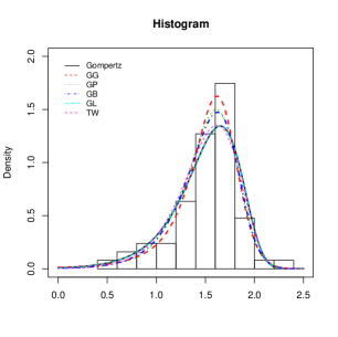
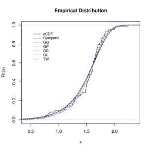
Figure 7: Plots (density and distribution) of fitted Gompertz, GG, GP, GB, GL and TW distributions for the data set.

Figure 8: QQ plots of the Gompertz, GG, GP, GB, GL and TW models.

Table 5: Parameter estimates (with std.), K-S statistic, p-value, AIC, AICC and BIC for the data set.

Dis.	Gompertz	GG	GP	GB	GL	TW
$\hat{\beta}$ (std.)	0.0088 (0.001)	0.8023 (0.772)	0.0006 (0.001)	0.0013 (0.001)	0.0088 (0.011)	-13.9192(—–)
$\hat{\gamma}$ (std.)	3.6474 (0.069)	1.3082 (0.586)	4.4611 (0.566)	4.2406 (0.404)	3.6474 (0.593)	11.8558 (9.795)
$\hat{\theta}$ (std.)	—	-58.8912 (91.83)	5.5965 (3.224)	1.8740 (1.268)	0.0001 (1.310)	-1.5934 (2.637)
$-\log(L)$	14.8081	12.2288	12.8702	13.0212	14.8067	14.2853
K-S	0.1268	0.0962	0.1207	0.1217	0.1267	0.0001
p-value	0.2636	0.6040	0.3177	0.3085	0.2636	0.9869
AIC	33.6162	30.4576	31.7404	32.0424	35.6134	34.5712
AICC	33.8162	30.8644	32.1472	32.4491	36.0202	34.9774
BIC	37.9025	36.8870	38.1698	38.4718	42.0428	40.9999

Appendix

A.

Here, we give the proof of Theorems 5.1, 5.2, and 5.3. Consider $p_{i}=\exp(-\frac{1}{\gamma}(e^{-\beta x_{i}}-1))$.

A.1

Let $w_{1}\left(\beta;\gamma,\theta,{\boldsymbol{x}}\right)=\sum^{n}_{i=1}\frac{\theta p^{\beta}_{i}\log(p_{i})C^{\prime\prime}(\theta p^{\beta}_{i})}{C^{\prime}(\theta p^{\beta}_{i})}=\frac{\partial}{\partial\beta}\sum^{n}_{i=1}\log(C^{\prime}(\theta p^{\beta}_{i}))$. Then, $w_{1}\left(\beta;\gamma,\theta,{\boldsymbol{x}}\right)$ is strictly increasing in $\beta$ and

$${\mathop{\lim}_{\beta\rightarrow 0^{+}}w_{1}}\left(\beta;\gamma,\theta,{\boldsymbol{x}}\right)=\frac{\theta C^{\prime\prime}(\theta)}{C^{\prime}(\theta)}\sum^{n}_{i=1}\log\left(p_{i}\right),\ \ \ \ \ \ \ \ \ \ {\mathop{\lim}_{\beta\rightarrow\infty}}w_{1}\left(\beta;\gamma,\theta,{\boldsymbol{x}}\right)=0.$$

Therefore,

$${\mathop{\lim}_{\beta\rightarrow 0^{+}}{{\rm g}}_{1}}\left(\beta;\gamma,\theta,{\boldsymbol{x}}\right)=\infty,\ \ \ \ \ \ \ \ {\mathop{\lim}_{\beta\rightarrow\infty}{\rm g}_{1}}\left(\beta;\gamma,\theta,{\boldsymbol{x}}\right)=\sum^{n}_{i{\rm=1}}\log\left(p_{i}\right)<0.$$

Also,

$${\rm g}_{1}\left(\beta;\gamma,\theta,{\boldsymbol{x}}\right)<\frac{n}{\beta}+\sum^{n}_{i=1}\log\left(p_{i}\right),\ \ \ \ \ \ {\rm g}_{1}\left(\beta;\gamma,\theta,{\boldsymbol{x}}\right)>\frac{n}{\beta}+\left(\frac{\theta C^{\prime\prime}\left(\theta\right)}{C^{\prime}\left(\theta\right)}+1\right)\sum^{n}_{i=1}\log\left(p_{i}\right).$$

Therefore, ${\rm g}_{1}\left(\beta;\gamma,\theta,{\boldsymbol{x}}\right)<0$ when $\frac{n}{\beta}+\sum^{n}_{i=1}\log\left(p_{i}\right)<0$, and ${\rm g}_{1}\left(\beta;\gamma,\theta,{\boldsymbol{x}}\right)>0$ when $\frac{n}{\beta}+\left(\frac{\theta C^{\prime\prime}(\theta)}{C^{\prime}(\theta)}+1\right)\sum^{n}_{i=1}\log\left(p_{i}\right)>0$. Hence, the proof is completed.

A.2

It can be easily shown that

$${\mathop{\lim}_{\gamma\rightarrow 0^{+}}{\rm g_{2}}(\gamma;\beta,\theta,{\boldsymbol{x}})}=n\bar{x}-\frac{\beta}{2}\sum^{n}_{i=1}{x^{2}_{i}\left(1+\frac{\theta e^{-\beta x_{i}}C^{\prime\prime}\left(\theta e^{-\beta x_{i}}\right)}{C^{\prime}\left(\theta e^{-\beta x_{i}}\right)}\right)},\;\ \ \ \ {\mathop{\lim}_{\gamma\rightarrow+\infty}{\rm g_{2}}(\gamma;\beta,\theta,{\boldsymbol{x}})}=-\infty.$$

Since the limits have different signs, the equation ${\rm g_{2}}(\gamma;\beta,\theta,{\boldsymbol{x}})=0$ has at least one root with respect to $\gamma$ for fixed values $\beta$ and $\theta$. The proof is completed.

A.3

(i) For GP, it is clear that

$${\mathop{\lim}_{\theta\rightarrow 0^{+}}}{\rm g}_{3}\left(\theta;\beta,\gamma,{\boldsymbol{x}}\right)=\sum\limits_{i=1}^{n}t_{i}-\frac{n}{2},\qquad\qquad{\mathop{\lim}_{\theta\rightarrow\infty}}{\rm g}_{3}\left(\theta;\beta,\gamma,{\boldsymbol{x}}\right)=-\infty.$$

Therefore, the equation ${\rm g}_{3}\left(\theta;\beta,\gamma,{\boldsymbol{x}}\right)=0$ has at least one root for $\theta>0$, if $\sum\limits_{i=1}^{n}t_{i}-\frac{n}{2}>0$ or $\sum\limits_{i=1}^{n}t_{i}>\frac{n}{2}$.
(ii) For GG, it is clear that

$${\mathop{\lim}_{\theta\rightarrow\infty}}{\rm g}_{3}\left(\theta;\beta,\gamma,{\boldsymbol{x}}\right)=-\infty,\qquad\qquad{\mathop{\lim}_{\theta\rightarrow 0^{+}}}{\rm g}_{3}\left(\theta;\beta,\gamma,{\boldsymbol{x}}\right)=-n+2\sum\limits_{i=1}^{n}t_{i}.$$

Therefore, the equation ${\rm g}_{3}\left(\theta;\beta,\gamma,{\boldsymbol{x}}\right)=0$ has at least one root for $0<\theta<1$, if $-n+2\sum\limits_{i=1}^{n}t_{i}>0$ or $\sum\limits_{i=1}^{n}t_{i}>\frac{n}{2}$.
(iii) For GL, it is clear that

$${\mathop{\lim}_{\theta\rightarrow 0^{+}}}{\rm g}_{3}\left(\theta;\beta,\gamma,{\boldsymbol{x}}\right)=\sum\limits_{i=1}^{n}t_{i}-\frac{n}{2},\qquad\qquad{\mathop{\lim}_{\theta\rightarrow 1^{-}}}{\rm g}_{3}\left(\theta;\beta,\gamma,{\boldsymbol{x}}\right)=-\infty.$$

Therefore, the equation ${\rm g}_{3}\left(\theta;\beta,\gamma,{\boldsymbol{x}}\right)=0$ has at least one root for $0<\theta<1$, if $\sum\limits_{i=1}^{n}t_{i}-\frac{n}{2}>0$ or $\sum\limits_{i=1}^{n}t_{i}>\frac{n}{2}$.
(iv) It is clear that

$${\mathop{\lim}_{p\rightarrow 0^{+}}}{\rm g}_{3}\left(p;\beta,\gamma,{\boldsymbol{x}}\right)=\sum\limits_{i=1}^{n}t_{i}(m-1)-\frac{n(m-1)}{2},\quad\quad{\mathop{\lim}_{p\rightarrow 1^{-}}}{\rm g}_{3}\left(p;\beta,\gamma,{\boldsymbol{x}}\right)=\sum\limits_{i=1}^{n}\frac{-m+1+mt_{i}}{t_{i}}.$$

Therefore, the equation ${\rm g}_{3}\left(p;\beta,\gamma,{\boldsymbol{x}}\right)=0$ has at least one root for $0<p<1$, if $\sum\limits_{i=1}^{n}t_{i}(m-1)-\frac{n(m-1)}{2}>0$ and $\sum\limits_{i=1}^{n}\frac{-m+1+mt_{i}}{t_{i}}<0$ or $\sum\limits_{i=1}^{n}t_{i}>\frac{n}{2}$ and $\sum\limits_{i=1}^{n}t_{i}^{-1}>\frac{nm}{1-m}$.

B.

Consider

$$t_{i}=e^{-\frac{\beta}{\gamma}(e^{\gamma x_{i}}-1)},\qquad b_{i}=\frac{\partial t_{i}}{\partial\gamma}=t_{i}d_{i},\qquad d_{i}=\frac{\partial\log(t_{i})}{\partial\gamma}=\frac{1}{\gamma}(-\log(t_{i})+\gamma x_{i}\log(t_{i})-\beta x_{i}),$$

$$q_{i}=\frac{\partial d_{i}}{\partial\gamma}=d_{i}(x_{i}-\frac{2}{\gamma})+\frac{x_{i}}{\gamma}\log(t_{i}),\qquad A_{2i}=\frac{C^{\prime\prime}(\theta t_{i})}{C^{\prime}(\theta t_{i})},\qquad A_{3i}=\frac{C^{\prime\prime\prime}(\theta t_{i})}{C^{\prime}(\theta t_{i})}.$$

Then, the elements of $3\times 3$ observed information matrix $I_{n}(\Theta)$ are given by

$$I_{\beta\beta} = \frac{\partial^{2}l_{n}}{\partial\beta^{2}}=-\frac{n}{\beta^{2}}+\frac{\theta}{\beta^{2}}\sum\limits_{i=1}^{n}t_{i}(\log(t_{i}))^{2}A_{2i}+\frac{\theta^{2}}{\beta^{2}}\sum\limits_{i=1}^{n}t_{i}^{2}(\log(t_{i}))^{2}A_{3i}-\frac{\theta^{2}}{\beta^{2}}\sum\limits_{i=1}^{n}t_{i}^{2}(\log(t_{i}))^{2}A_{2i}^{2},$$

$$I_{\beta\gamma} = \frac{\partial^{2}l_{n}}{\partial\beta\partial\gamma}=\frac{1}{\beta}\sum\limits_{i=1}^{n}d_{i}+\frac{\theta}{\beta}\sum\limits_{i=1}^{n}b_{i}\log(t_{i})A_{2i}+\frac{\theta}{\beta}\sum\limits_{i=1}^{n}b_{i}A_{2i}$$

$$+\frac{\theta^{2}}{\beta}\sum\limits_{i=1}^{n}b_{i}t_{i}\log(t_{i})A_{3i}-\frac{\theta^{2}}{\beta}\sum\limits_{i=1}^{n}b_{i}t_{i}\log(t_{i})A_{2i}^{2},$$

$$I_{\beta\theta} = \frac{\partial^{2}l_{n}}{\partial\beta\partial\theta}=\frac{1}{\beta}\sum\limits_{i=1}^{n}t_{i}\log(t_{i})A_{2i}+\frac{\theta}{\beta}\sum\limits_{i=1}^{n}t_{i}^{2}\log(t_{i})A_{3i}-\frac{\theta}{\beta}\sum\limits_{i=1}^{n}t_{i}^{2}\log(t_{i})A_{2i}^{2},$$

$$I_{\gamma\gamma} = \frac{\partial^{2}l_{n}}{\partial\gamma^{2}}=\sum\limits_{i=1}^{n}q_{i}+\theta\sum\limits_{i=1}^{n}(b_{i}d_{i}+t_{i}q_{i})A_{2i}+\theta^{2}\sum\limits_{i=1}^{n}b_{i}^{2}A_{3i}-\theta^{2}\sum\limits_{i=1}^{n}b_{i}^{2}A_{2i}^{2},$$

$$I_{\gamma\theta} = \frac{\partial^{2}l_{n}}{\partial\theta\partial\gamma}=\sum\limits_{i=1}^{n}b_{i}A_{2i}+\theta\sum\limits_{i=1}^{n}t_{i}b_{i}A_{3i}-\theta\sum\limits_{i=1}^{n}t_{i}b_{i}A_{2i}^{2},$$

$$I_{\theta\theta} = \frac{\partial^{2}l_{n}}{\partial\theta^{2}}=-\frac{n}{\theta^{2}}+\sum\limits_{i=1}^{n}t_{i}^{2}A_{3i}-\sum\limits_{i=1}^{n}t_{i}^{2}A_{2i}^{2}-\frac{nC^{\prime\prime}(\theta)}{C(\theta)}+\frac{n(C^{\prime}(\theta))^{2}}{(C(\theta))^{2}}.$$

References

- Adamidis et al. (2005) Adamidis, K., Dimitrakopoulou, T., and Loukas, S. (2005). On an extension of the exponential–geometric distribution. Statistics and Probability Letters, 73(3):259–269.
- Adamidis and Loukas (1998) Adamidis, K. and Loukas, S. (1998). A lifetime distribution with decreasing failure rate. Statistics and Probability Letters, 39(1):35–42.
- Barreto-Souza et al. (2010) Barreto-Souza, W., Santos, A. H. S., and Cordeiro, G. M. (2010). The beta generalized exponential distribution. Journal of Statistical Computation and Simulation, 80(2):159–172.
- Cancho et al. (2011) Cancho, V. G., Louzada-Neto, F., and Barriga, G. D. C. (2011). The Poisson–exponential lifetime distribution. Computational Statistics and Data Analysis, 55(1):677–686.
- Casella and Berger (2001) Casella, G. and Berger, R. (2001). Statistical Inference. Duxbury, Pacific Grove, California, USA.
- Chahkandi and Ganjali (2009) Chahkandi, M. and Ganjali, M. (2009). On some lifetime distributions with decreasing failure rate. Computational Statistics and Data Analysis, 53(12):4433–4440.
- Dempster et al. (1977) Dempster, A. P., Laird, N. M., and Rubin, D. B. (1977). Maximum likelihood from incomplete data via the EM algorithm. Journal of the Royal Statistical Society. Series B (Methodological), 39(1):1–38.
- Flores et al. (2011) Flores, J., Borges, P., Cancho, V. G., and Louzada, F. (2011). The complementary exponential power series distribution. Brazilian Journal of Probability and Statistics, (accepted).
- Johnson et al. (2005) Johnson, N. L., Kemp, A. W., and Kotz, S. (2005). Univariate discrete distributions. Wiley-Interscience, third edition.
- Kuş (2007) Kuş, C. (2007). A new lifetime distribution. Computational Statistics and Data Analysis, 51(9):4497–4509.
- Lenart (2012) Lenart, A. (2012). The moments of the Gompertz distribution and maximum likelihood estimation of its parameters. Scandinavian Actuarial Journal, 10.1080/03461238.2012.687697.
- Louis (1982) Louis, T. A. (1982). Finding the observed information matrix when using the EM algorithm. Journal of the Royal Statistical Society. Series B (Methodological), 44(2):226–233.
- Louzada et al. (2011) Louzada, F., Roman, M., and Cancho, V. G. (2011). The complementary exponential geometric distribution: Model, properties, and a comparison with its counterpart. Computational Statistics and Data Analysis, 55(8):2516–2524.
- Mahmoudi and Jafari (2012) Mahmoudi, E. and Jafari, A. A. (2012). Generalized exponential–power series distributions. Computational Statistics and Data Analysis, 56(12):4047–4066.
- Marshall and Olkin (1997) Marshall, A. W. and Olkin, I. (1997). A new method for adding a parameter to a family of distributions with application to the exponential and Weibull families. Biometrika, 84(3):641–652.
- Morais and Barreto-Souza (2011) Morais, A. L. and Barreto-Souza, W. (2011). A compound class of Weibull and power series distributions. Computational Statistics and Data Analysis, 55(3):1410–1425.
- Noack (1950) Noack, A. (1950). A class of random variables with discrete distributions. The Annals of Mathematical Statistics, 21(1):127–132.
- Shannon (1948) Shannon, C. (1948). A mathematical theory of communication. Bell System Technical Journal, 27:379–432.
- Smith and Naylor (1987) Smith, R. L. and Naylor, J. C. (1987). A comparison of maximum likelihood and bayesian estimators for the three-parameter Weibull distribution. Applied Statistics, 36(3):358–369.
- Tahmasbi and Rezaei (2008) Tahmasbi, R. and Rezaei, S. (2008). A two-parameter lifetime distribution with decreasing failure rate. Computational Statistics and Data Analysis, 52(8):3889–3901.