Mass-critical inverse Strichartz theorems for 1d Schrödinger operators

Abstract.

We prove inverse Strichartz theorems at $L^{2}$ regularity for a family of Schrödinger evolutions in one space dimension. Prior results rely on spacetime Fourier analysis and are limited to the translation-invariant equation $i\partial_{t}u=-\tfrac{1}{2}\Delta u$. Motivated by applications to the mass-critical Schrödinger equation with external potentials (such as the harmonic oscillator), we use a physical space approach.

1. Introduction

In this paper, we prove an inverse Strichartz theorem for certain Schrödinger evolutions on the real line with $L^{2}$ initial data. Recall that solutions to the linear Schrödinger equation

(1.1) $$i\partial_{t}u=-\tfrac{1}{2}\Delta u\quad\text{with}\quad u(0,\cdot)\in L^{2}(\mathbf{R}^{d}),$$

satisfy the Strichartz inequality

(1.2) $$\|u\|_{L^{\frac{2(d+2)}{2}}_{t,x}(\mathbf{R}\times\mathbf{R}^{d})}\leq C\|u(0,\cdot)\|_{L^{2}(\mathbf{R}^{d})}.$$

In this translation-invariant setting, it was proved that if $u$ comes close to saturating the above inequality, then the initial data $u(0)$ must exhibit some “concentration”; see [CK07, MV98, MVV99, BV07]. We seek analogues of this result when the right side of (1.1) is replaced by a more general Schrödinger operator $-\tfrac{1}{2}\Delta+V(t,x)$.

Such refinements of the Strichartz inequality have provided a key technical tool in the study of the $L^{2}$-critical nonlinear Schrödinger equation

(1.3) $$i\partial_{t}u=-\tfrac{1}{2}\Delta u\pm|u|^{\frac{4}{d}}u\quad\text{with}\quad u(0,\cdot)\in L^{2}(\mathbf{R}^{d}).$$

The term “$L^{2}$-critical” or “mass-critical” refers to the property that the rescaling

$$u(t,x)\mapsto u_{\lambda}(t,x):=\lambda^{\frac{d}{2}}u(\lambda^{2}t,\lambda x),\quad\lambda>0,$$

preserves both the class of solutions and the conserved mass $M[u]:=\|u(t)\|_{L^{2}}^{2}=\|u(0)\|_{L^{2}}^{2}.$ An inverse theorem for (1.2) begets profile decompositions that underpin the large data theory by revealing how potential blowup solutions may concentrate. The reader may consult for instance the notes [KV13] for a more detailed account of this connection. The initial-value problem (1.3) was shown to be globally wellposed in [Dod12, Dodb, Doda, Dod15, KTV09, KVZ08, TVZ07].

Characterizing near-optimizers of the inequality (1.2) involves significant technical challenges due to the presence of noncompact symmetries. Besides invariance under rescaling and translations in space and time, the inequality also possesses Galilean invariance

$$u(t,x)\mapsto u_{\xi_{0}}(t,x):=e^{i[x\xi_{0}-\frac{1}{2}t|\xi_{0}|^{2}]}u(t,x-t\xi_{0}),\quad u_{\xi_{0}}(0)=e^{ix\xi_{0}}u(0),\quad\xi_{0}\in\mathbf{R}^{d}.$$

Because of this last degeneracy, the $L^{2}$-critical setting is much more delicate compared to variants of (1.2) with higher regularity Sobolev norms on the right side, such as the energy-critical analogue

(1.4) $$\|u\|_{L^{\frac{2(d+2)}{d-2}}_{t,x}(\mathbf{R}\times\mathbf{R}^{d})}\leq C\|\nabla u(0,\cdot)\|_{L^{2}(\mathbf{R}^{d})}.$$

In particular, Littlewood-Paley theory has little use when seeking an inverse to (1.2) because $u(0)$ can concentrate anywhere in frequency space, not necessarily near the origin. The works cited above use spacetime orthogonality arguments and appeal to Fourier restriction theory, such as Tao’s bilinear estimate for paraboloids (when $d\geq 3$) [Tao03].

Ultimately, we wish to consider the large data theory for the equation

(1.5) $$i\partial_{t}u=-\frac{1}{2}\Delta u+Vu\pm|u|^{\frac{4}{d}}u,\quad u(0,\cdot)\in L^{2}(\mathbf{R}^{d}),$$

where $V(x)$ is a real-valued potential. The main example we have in mind is the harmonic oscillator $V=\sum_{j}\omega_{j}^{2}x_{j}^{2}$, which has obvious physical relevance and arises in the study of Bose-Einstein condensates [Zha00]. Although the scaling symmetry is broken, solutions initially concentrated at a point are well-approximated for short times by (possibly modulated) solutions to the genuinely scale-invariant mass-critical equation (1.3). As described in Lemma 2.5 below, the harmonic oscillator also admits a more complicated analogue of Galilean invariance. This is related to the fact that $u$ solves equation (1.3) iff its Lens transform $\mathcal{L}u$ satisfies equation (1.5) with $V=\tfrac{1}{2}|x|^{2}$, where

$$\mathcal{L}u(t,x):=\tfrac{1}{(\cos t)^{d/2}}u\Bigl{(}\tan t,\tfrac{x}{\cos t}\Bigr{)}e^{-\frac{i|x|^{2}\tan t}{2}}.$$

The energy-critical counterpart to (1.5) with $V=\tfrac{1}{2}|x|^{2}$ was recently studied by the first author [Jao16].

While the Lens transform may be inverted to deduce global wellposedness for the mass-critical harmonic oscillator when $\omega_{j}\equiv\tfrac{1}{2}$, this miraculous connection with equation (1.3) evaporates as soon as the $\omega_{j}$ are not all equal. Studying the equation in greater generality therefore requires a more robust line of attack, such as the concentration-compactness and rigidity paradigm. To implement that strategy one needs appropriate inverse $L^{2}$ Strichartz estimates. This is no small matter since the Fourier-analytic techniques underpinning the proofs of the constant-coefficient theorems—most notably, Fourier restriction estimates—are ill-adapted to large variable-coefficient perturbations.

We present a different approach to these inverse estimates in one space dimension. By eschewing Fourier analysis for physical space arguments, we can treat a family of Schrödinger operators that includes the free particle and the harmonic oscillator. Moreover, our potentials are allowed to depend on time.

1.1. The setup

Consider a (possibly time-dependent) Schrödinger operator on the real line

$$H(t)=-\tfrac{1}{2}\partial^{2}_{x}+V(t,x)\quad x\in\mathbf{R},$$

and assume $V$ is a subquadratic potential. Specifically, we require that $V$ satisfies the following hypotheses:

• For each $k\geq 2$, there exists there exists $M_{k}<\infty$ so that

  (1.6) $$\|V(t,x)\|_{L^{\infty}_{t}L^{\infty}_{x}(|x|\leq 1)}+\|\partial^{k}_{x}V(t,x)\|_{L^{\infty}_{t,x}}+\|\partial^{k}_{x}\partial_{t}V(t,x)\|_{L^{\infty}_{t,x}}\leq M_{k}.$$

• There exists some $\varepsilon>0$ so that

  (1.7) $$|\langle x\rangle^{1+\varepsilon}\partial^{3}_{x}V|+|\langle x\rangle^{1+\varepsilon}\partial^{3}_{x}\partial_{t}V|\in L^{\infty}_{t,x}.$$

  By the fundamental theorem of calculus, this implies that the second derivative $\partial^{2}_{x}V(t,x)$ converges as $x\to\pm\infty$. Here and in the sequel, we write $\langle x\rangle:=(1+|x|^{2})^{1/2}$.

Note that the potentials $V=0$ and $V=\tfrac{1}{2}x^{2}$ both fall into this class.

The first set of conditions on the space derivatives of $V$ are quite natural in view of classical Fourier integral operator constructions, from which one can deduce dispersive and Strichartz estimates; see Theorem 2.3. We also need some time regularity of solutions for our spacetime orthogonality arguments. However, the decay hypothesis on the third derivative $\partial^{3}_{x}V$ is technical; see the discussion surrounding Lemma 5.1 below.

The propagator $U(t,s)$ for such Hamiltonians is known to obey Strichartz estimates at least locally in time:

(1.8) $$\|U(t,s)f\|_{L^{6}_{t,x}(I\times\mathbf{R})}\lesssim_{I}\|f\|_{L^{2}(\mathbf{R})}$$

for any compact interval $I$ and any fixed $s\in\mathbf{R}$; see Corollary 2.4. Note that $U(t,s)=e^{-i(t-s)H}$ is a one-parameter group if one assumes that $V=V(x)$ is time-independent, but our methods do not require this assumption.

Our main result asserts that if the left side is nontrivial relative to the right side, then the evolution of initial data must contain a “bubble” of concentration. Such concentration will be detected by probing the solution with suitably scaled, translated, and modulated test functions.

For $\lambda>0$ and $(x_{0},\xi_{0})\in T^{*}\mathbf{R}\cong\mathbf{R}_{x}\times\mathbf{R}_{\xi}$, define the scaling and phase space translation operators

$$S_{\lambda}f(x)=\lambda^{-1/2}f(\lambda^{-1}x)\quad\text{and}\quad\pi(x_{0},\xi_{0})f(x)=e^{i(x-x_{0})\xi_{0}}f(x-x_{0}).$$

Let $\psi$ denote a real even Schwartz function with $\|\psi\|_{2}=(2\pi)^{-1/2}$. Its phase space translate $\pi(x_{0},\xi_{0})\psi$ is localized in space near $x_{0}$ and in frequency near $\xi_{0}$.

Theorem 1.1.

There exists $\beta>0$ such that if $0<\varepsilon\leq\|U(t,0)f\|_{L^{6}([-\frac{1}{2},\frac{1}{2}]\times\mathbf{R})}$ and $\|f\|_{L^{2}}\leq A$, then

$$\sup_{z\in T^{*}\mathbf{R},\ 0<\lambda\leq 1,\ |t|\leq 1/2}|\langle\pi(z)S_{\lambda}\psi,U(t,0)f\rangle_{L^{2}(\mathbf{R})}|\geq C\varepsilon(\tfrac{\varepsilon}{A})^{\beta}$$

for some constant $C$ depending on the seminorms in (1.6) and (1.7).

By repeatedly applying the following corollary, one can obtain a linear profile decomposition. For simplicity, we state it assuming the potential is time-independent (so that $U(t,0)=e^{-itH}$).

Corollary 1.2.

Let $\{f_{n}\}\subset L^{2}(\mathbf{R})$ be a sequence such that $0<\varepsilon\leq\|e^{-itH}f_{n}\|_{L^{6}_{t,x}([-\frac{1}{2},\frac{1}{2}]\times\mathbf{R})}$ and $\|f\|_{L^{2}}\leq A$ for some constants $A,\varepsilon>0$. Then, after passing to a subsequence, there exist a sequence of parameters

$$\{(\lambda_{n},t_{n},z_{n})\}_{n}\subset(0,1]\times[-1/2,1/2]\times T^{*}\mathbf{R}$$

and a function $0\neq\phi\in L^{2}$ such that,

$$S_{\lambda_{n}}^{-1}\pi(z_{n})^{-1}e^{-it_{n}H}f_{n}\rightharpoonup\phi\text{ in }L^{2}$$

(1.9) $$\|\phi\|_{L^{2}}\gtrsim\varepsilon(\tfrac{\varepsilon}{A})^{\beta}.$$

Further,

(1.10) $$\|f_{n}\|_{2}^{2}-\|f_{n}-e^{it_{n}H}\pi(z_{n})S_{\lambda_{n}}\phi\|_{2}^{2}-\|e^{it_{n}H}\pi(z_{n})S_{\lambda_{n}}\phi\|_{2}^{2}\to 0.$$

Proof.

By Theorem 1.1, there exist $(\lambda_{n},t_{n},z_{n})$ such that $|\langle\pi(z_{n})S_{\lambda_{n}}\psi,e^{-it_{n}H}f_{n}\rangle|\gtrsim\varepsilon(\tfrac{\varepsilon}{A})^{\beta}$. As the sequence $S_{\lambda_{n}}^{-1}\pi(z_{n})^{-1}e^{-it_{n}H}f_{n}$ is bounded in $L^{2}$, it has a weak subsequential limit $\phi\in L^{2}$. Passing to this subsequence, we have

$$\|\phi\|_{2}\gtrsim|\langle\psi,\phi\rangle|=\lim_{n\to\infty}|\langle\psi,S_{\lambda_{n}}^{-1}\pi(z_{n})^{-1}e^{-it_{n}H}f_{n}\rangle|\gtrsim\varepsilon(\tfrac{\varepsilon}{A})^{\beta}.$$

To obtain (1.10), write the left side as

$$\begin{split}2\operatorname{Re}\langle f_{n}-e^{it_{n}H}\pi(z_{n})S_{\lambda_{n}}\phi,e^{it_{n}H}\pi(z_{n})S_{\lambda_{n}}\phi\rangle=2\operatorname{Re}\langle S_{\lambda_{n}}^{-1}\pi(z_{n})^{-1}e^{-it_{n}H}f_{n}-\phi,\phi\rangle\to 0,\end{split}$$

by the definition of $\phi$. ∎

The restriction to a compact time interval in the above statements is dictated by the generality of our hypotheses. For a generic subquadratic potential, the $L^{6}_{t,x}$ norm of a solution need not be finite on $\mathbf{R}_{t}\times\mathbf{R}_{x}$. For example, solutions to the harmonic oscillator (for which $V(x)=\frac{1}{2}x^{2}$) are periodic in time. However, the conclusions may be strengthened in some cases. In particular, our methods specialize to the case $V=0$ to yield

Theorem 1.3.

If $0<\varepsilon\leq\|e^{\frac{it\Delta}{2}}f\|_{L^{6}_{t,x}(\mathbf{R}\times\mathbf{R})}\lesssim\|f\|_{L^{2}}=A$, then

$$\sup_{z\in T^{*}\mathbf{R},\ \lambda>0,\ t\in\mathbf{R}}|\langle\pi(z)S_{\lambda}\psi,e^{\frac{it\Delta}{2}}f\rangle|\gtrsim\varepsilon(\tfrac{\varepsilon}{A})^{\beta}.$$

This yields an analogue to Corollary 1.2, which can be used to derive a linear profile decomposition for the one dimensional free particle. Such a profile decomposition was obtained originally by Carles and Keraani [CK07] using different methods.

1.2. Ideas of proof

We shall assume in the sequel that the initial data $f$ is Schwartz. This assumption will justify certain applications of Fubini’s theorem and may be removed a posteriori by an approximation argument. Further, we prove the theorem with the time interval $[-\tfrac{1}{2},\tfrac{1}{2}]$ replaced by $[-\delta_{0},\delta_{0}]$, where $\delta_{0}$ is furnished by Theorem 2.3 according to the seminorms $M_{k}$ of the potential. Indeed, the interval $[-\tfrac{1}{2},\tfrac{1}{2}]$ can then be tiled by subintervals of length $\delta_{0}$.

Given these preliminary reductions, we describe the main ideas of the proof of Theorem 1.1. Our goal is to locate the parameters describing a concentration bubble in the evolution of the initial data. The relevant parameters are a length scale $\lambda_{0}$, spatial center $x_{0}$, frequency center $\xi_{0}$, and a time $t_{0}$ describing when the concentration occurs. Each parameter is associated with a noncompact symmetry or approximate symmetry of the Strichartz inequality. For instance, when $V=0$ or $V=\tfrac{1}{2}x^{2}$, both sides of (1.8) are preserved by translations $f\mapsto f(\cdot-x_{0})$ and modulations $f\mapsto e^{i(\cdot)\xi_{0}}f$ of the initial data, while more general $V$ admit an approximate Galilean invariance; see Lemma 2.5 below.

The existing approaches to inverse Strichartz inequalities for the free particle can be roughly summarized as follows. First, one uses Fourier analysis to isolate a scale $\lambda_{0}$ and frequency center $\xi_{0}$. For example, Carles-Keraani prove in their Proposition 2.1 that for some $1<p<2$,

$$\|e^{it\partial_{x}^{2}}f\|_{L^{6}_{t,x}(\mathbf{R}\times\mathbf{R})}\lesssim_{p}\Bigl{(}\sup_{J}|J|^{\frac{1}{2}-\frac{1}{p}}\|\hat{f}\|_{L^{p}(J)}\Bigr{)}^{1/3}\|f\|_{L^{2}(\mathbf{R})},$$

where $J$ ranges over all intervals and $\hat{f}$ is the Fourier transform of $f$. Then one uses a separate argument to determine $x_{0}$ and $t_{0}$. This strategy ultimately relies on the fact that the propagator for the free particle is diagonalized by the Fourier transform.

One does not enjoy that luxury with general Schrödinger operators as the momenta of particles may vary with time and in a position-dependent manner. Thus it is natural to consider the position and frequency parameters together in phase space. To this end, we use a wavepacket decomposition as a partial substitute for the Fourier transform. Unlike the Fourier transform, however, the wavepacket transform requires that one first chooses a length scale. This is not entirely trivial because the Strichartz inequality (1.8) which we are trying to invert has no intrinsic length scale; the rescaling

$$f\mapsto\lambda^{-d/2}f(\lambda^{-1}\cdot),\ 0<\lambda\ll 1$$

preserves both sides of the inequality exactly when $V=0$ and at least approximately for subquadratic potentials $V$.

We obtain the parameters in a different order. Using a direct physical space argument, we show that if $u(t,x)$ is a solution with nontrivial $L^{6}_{t,x}$ norm, then there exists a time interval $J$ such that $u$ is large in $L^{q}_{t,x}(J\times\mathbf{R})$ for some $q<6$. Unlike the $L^{6}_{t,x}$ norm, the $L^{q}_{t,x}$ is not scale-invariant, hence the interval $J$ identifies a significant time $t_{0}$ and physical scale $\lambda_{0}=\sqrt{|J|}$. By an interpolation and rescaling argument, we then reduce matters to a refined $L^{2}_{x}\to L^{4}_{t,x}$ estimate. This is then proved using a wavepacket decomposition, integration by parts, and analysis of bicharacteristics, revealing the parameters $x_{0}$ and $\xi_{0}$ simultaneously.

This paper is structured as follows. Section 2 collects some preliminary definitions and lemmas. The heart of the argument is presented in Sections 3 and 4. As the identification of a time interval works in any number of space dimensions, Section 3 is written for a general subquadratic Schrödinger operator on $\mathbf{R}^{d}$. In fact the argument there applies to any linear propagator that satisfies the dispersive estimate. In the later sections we specialize to $d=1$.

Further insights seem to be needed in two or more space dimensions. A naive attempt to extend our methods to higher dimensions would require us to prove a refined $L^{p}$ estimate for some $2<p<4$; our arguments in this paper exploit the fact that $4$ is an even integer. There is also a more conceptual barrier: while a timescale should serve as a proxy for one spatial scale, there may a priori exist more than one interesting physical scale in higher dimensions. For instance, the nonelliptic Schrödinger equation

$$i\partial_{t}u=-\partial_{x}\partial_{y}u$$

in two dimensions satisfies the Strichartz estimate (1.2) and admits the scaling symmetry $u\mapsto u(t,\lambda x,\lambda^{-1}y)$ in addition to the usual one. A refinement of the Strichartz inequality for this particular example was obtained using Fourier-analytic methods by Rogers and Vargas [RV06]. Any higher-dimensional generalization of our methods must somehow distinguish the elliptic and nonelliptic cases.

Acknowledgements

This work was partially supported by NSF grants DMS-1265868 (PI R. Killip), DMS-1161396, and DMS-1500707 (both PI M. Visan).

2. Preliminaries

2.1. Phase space transforms

We briefly recall the (continuous) wavepacket decomposition; see for instance [Fol89]. Fix a real, even Schwartz function $\psi\in\mathcal{S}(\mathbf{R}^{d})$ with $\|\psi\|_{L^{2}}=(2\pi)^{-d/2}$. For a function $f\in L^{2}(\mathbf{R}^{d})$ and a point $z=(x,\xi)\in T^{*}\mathbf{R}^{d}=\mathbf{R}^{d}_{x}\times\mathbf{R}^{d}_{\xi}$ in phase space, define

$$Tf(z)=\int_{\mathbf{R}^{d}}e^{i(x-y)\xi}\psi(x-y)f(y)\,dy=\langle f,\psi_{z}\rangle_{L^{2}(\mathbf{R}^{d})}.$$

By taking the Fourier transform in the $x$ variable, we get

$$\mathcal{F}_{x}Tf(\eta,\xi)=\int_{\mathbf{R}^{d}}e^{-iy\eta}\hat{\psi}(\eta-\xi)f(y)\,dy=\hat{\psi}(\eta-\xi)\hat{f}(\eta).$$

Thus $T$ maps $\mathcal{S}(\mathbf{R}^{d})\to\mathcal{S}(\mathbf{R}^{d}\times\mathbf{R}^{d})$ and is an isometry $L^{2}(\mathbf{R}^{d})\to L^{2}(T^{*}\mathbf{R}^{d})$. The hypothesis that $\psi$ is even implies the adjoint formula

$$T^{*}F(y)=\int_{T^{*}\mathbf{R}^{d}}F(z)\psi_{z}(y)\,dz$$

and the inversion formula

$$f=T^{*}Tf=\int_{T^{*}\mathbf{R}^{d}}\langle f,\psi_{z}\rangle_{L^{2}(\mathbf{R}^{d})}\psi_{z}\,dz.$$

2.2. Estimates for bicharacteristics

Let $V(t,x)$ satisfy $\partial_{x}^{k}V(t,\cdot)\in L^{\infty}(\mathbf{R}^{d})$ for all $k\geq 2$, uniformly in $t$. The time-dependent symbol $h(t,x,\xi)=\tfrac{1}{2}|\xi|^{2}+V(t,x)$ defines a globally Lipschitz Hamiltonian vector field $\xi\partial_{x}-(\partial_{x}V)\partial_{\xi}$ on $T^{*}\mathbf{R}^{d}$, hence the flow map $\Phi(t,s):T^{*}\mathbf{R}^{d}\to T^{*}\mathbf{R}^{d}$ is well-defined for all $s$ and $t$. For $z=(x,\xi)$, write $z^{t}=(x^{t}(z),\xi^{t}(z))=\Phi(t,0)(z)$ denote the bicharacteristic starting from $z$ at time $0$.

Fix $z_{0},z_{1}\in T^{*}\mathbf{R}^{d}$. We obtain by integration

$$\begin{split}x_{0}^{t}-x_{1}^{t}&=x_{0}^{s}-x_{1}^{s}+(t-s)(\xi_{0}^{s}-\xi_{1}^{s})-\int_{s}^{t}(t-\tau)(\partial_{x}V(\tau,x_{0}^{\tau})-\partial_{x}V(\tau,x_{1}^{\tau}))\,d\tau\\ \xi_{0}^{t}-\xi_{1}^{t}&=\xi_{0}^{s}-\xi_{1}^{s}-\int_{s}^{t}(\partial_{x}V(\tau,x_{0}^{\tau})-\partial_{x}V(\tau,x_{1}^{\tau}))\,d\tau.\end{split}$$

As $|\partial_{x}V(\tau,x_{0}^{\tau})-\partial_{x}V(\tau,x_{1}^{\tau})|\leq\|\partial^{2}_{x}V\|_{L^{\infty}}|x_{0}^{\tau}-x_{1}^{\tau}|$, we have for $|t-s|\leq 1$

(2.1) $$\begin{split}&|x_{0}^{t}-x_{1}^{t}|\leq(|x_{0}^{s}-x_{1}^{s}|+|t-s||\xi_{0}^{s}-\xi_{1}^{s}|)e^{\|\partial_{x}^{2}V\|_{L^{\infty}}},\\ &|\xi_{0}^{t}-\xi_{1}^{t}-(\xi_{0}^{s}-\xi_{1}^{s})|\leq(|t-s||x_{0}^{s}-x_{1}^{s}|+|t-s|^{2}|\xi_{0}^{s}-\xi_{1}^{s}|)\|\partial^{2}_{x}V\|_{L^{\infty}}e^{\|\partial_{x}^{2}V\|_{L^{\infty}}},\\ &|x_{0}^{t}-x_{1}^{t}-(x_{0}^{s}-x_{1}^{s})-(t-s)(\xi_{0}^{s}-\xi_{1}^{s})|\leq(|t-s|^{2}|x_{0}^{s}-x_{1}^{s}|+|t-s|^{3}|\xi_{0}^{s}-\xi_{1}^{s}|)e^{\|\partial^{2}_{x}V\|_{L^{\infty}}}.\end{split}$$

In the sequel, we shall always assume that $|t-s|\leq 1$, and all implicit constants shall depend on $\partial^{2}_{x}V$ or finitely many higher derivatives. We also remark that this time restriction may be dropped if $\partial^{2}_{x}V\equiv 0$ (as in Theorem 1.3). The preceding computations immediately yield the following dynamical consequences:

Lemma 2.1.

Assume the preceding setup.

• There exists $\delta>0$, depending on $\|\partial_{x}^{2}V\|_{L^{\infty}}$, such that $|t-s|\leq\delta$ implies

  $$|x^{t}_{0}-x_{1}^{t}-(x_{0}^{s}-x_{1}^{s})-(t-s)(\xi_{0}^{s}-\xi_{1}^{s})|\leq\frac{1}{100}(|x_{0}^{s}-x_{1}^{s}|+|t-s||\xi_{0}^{s}-\xi_{1}^{s}|).$$

  Hence if $|x_{0}^{s}-x_{1}^{s}|\leq r$ and $C\geq 2$, then $|x_{0}^{t}-x_{1}^{t}|\geq Cr$ for $\tfrac{2Cr}{|\xi_{0}^{s}-\xi_{1}^{s}|}\leq|t-s|\leq\delta$. Informally, two particles colliding with sufficiently large relative velocity will interact only once during a length $\delta$ time interval.

• With $\delta$ and $C$ as above, if $|x_{0}^{s}-x_{1}^{s}|\leq r$, then

  $$|\xi_{0}^{t}-\xi_{1}^{t}-(\xi_{0}^{s}-\xi_{1}^{s})|\leq\min\Bigl{(}\delta,\frac{2Cr}{|\xi_{0}^{s}-\xi_{1}^{s}|}\Bigr{)}Cr\|\partial^{2}_{x}V\|_{L^{\infty}}e^{\|\partial^{2}_{x}V\|_{L^{\infty}}}$$

  for all $t$ such that $|t-s|\leq\delta$ and $|x_{0}^{\tau}-x_{1}^{\tau}|\leq Cr$ for all $s\leq\tau\leq t$. That is, the relative velocity of two particles remains essentially constant during an interaction.

The following technical lemma will be used in Section 4.1.

Lemma 2.2.

There exists a constant $C>0$ so that if $Q_{\eta}=(0,\eta)+[-1,1]^{2d}$ and $r\geq 1$, then

$$\bigcup_{|t-t_{0}|\leq\min(|\eta|^{-1},1)}\Phi(t,0)^{-1}(z_{0}^{t}+rQ_{\eta})\subset\Phi(t_{0},0)^{-1}(z_{0}^{t_{0}}+CrQ_{\eta}).$$

In other words, if the bicharacteristic $z^{t}$ starting at $z\in T^{*}\mathbf{R}^{d}$ passes through the cube $z_{0}^{t}+rQ_{\eta}$ in phase space during some time window $|t-t_{0}|\leq\min(|\eta|^{-1},1)$, then it must lie in the dilate $z_{0}^{t_{0}}+CrQ_{\eta}$ at time $t_{0}$.

Proof.

If $z^{s}\in z_{0}^{s}+rQ_{\eta}$, then (2.1) and $|t-s|\leq\min(|\eta|^{-1},1)$ imply that

$$|x^{t}-x_{0}^{t}|\lesssim|x^{s}-x_{0}^{s}|+\min(|\eta|^{-1},1)(|\eta|+r)\lesssim r,$$

$$|\xi^{t}-\xi_{0}^{t}-(\xi^{s}-\xi_{0}^{s})|\lesssim r\min(|\eta|^{-1},1).$$

∎

2.3. The Schrödinger propagator

In this section we recall some facts regarding the quantum propagator for subquadratic potentials. First, we have the following oscillatory integral representation:

Theorem 2.3 (Fujiwara [Fuj79, Fuj80]).

Let $V(t,x)$ satisfy

$$M_{k}:=\|\partial^{k}_{x}V(t,x)\|_{L^{\infty}_{t,x}}+\|V(t,x)\|_{L^{\infty}_{t}L^{\infty}_{x}(|x|\leq 1)}<\infty$$

for all $k\geq 2$. There exists a constant $\delta_{0}>0$ such that for all $0<|t-s|\leq\delta_{0}$ the propagator $U(t,s)$ for $H=-\tfrac{1}{2}\Delta+V(t,x)$ has Schwartz kernel

$$U(t,s)(x,y)=\Bigl{(}\frac{1}{2\pi i(t-s)}\Bigr{)}^{d/2}a(t,s,x,y)e^{iS(t,s,x,y)},$$

where for each $m>0$ there is a constant $\gamma_{m}>0$ such that

$$\|a(t,s,x,y)-1\|_{C^{m}(\mathbf{R}^{d}_{x}\times\mathbf{R}^{d}_{y})}\leq\gamma_{m}|t-s|^{2}.$$

Moreover

$$S(t,s,x,y)=\frac{|x-y|^{2}}{2(t-s)}+(t-s)r(t,s,x,y),$$

with

$$|\partial_{x}r|+|\partial_{y}r|\leq C(M_{2})(1+|x|+|y|),$$

and for each multindex $\alpha$ with $|\alpha|\geq 2$, the quantity

$$C_{\alpha}=\|\partial^{\alpha}_{x,y}r(t,s,\cdot,\cdot)\|_{L^{\infty}}$$

is finite. The map $U(t,s):\mathcal{S}(\mathbf{R}^{d})\to\mathcal{S}(\mathbf{R}^{d})$ is a topological isomorphism, and all implicit constants depend on finitely many $M_{k}$.

Corollary 2.4 (Dispersive and Strichartz estimates).

If $V$ satisfies the hypotheses of the previous theorem, then $U(t,s)$ admits the fixed-time bounds

$$\|U(t,s)\|_{L^{1}_{x}(\mathbf{R}^{d})\to L^{\infty}_{x}(\mathbf{R}^{d})}\lesssim|t-s|^{-d/2}$$

whenever $|t-s|\leq\delta_{0}$. For any compact time interval $I$ and any exponents $(q,r)$ satisfying $2\leq q,r\leq\infty$, $\tfrac{2}{q}+\tfrac{d}{r}=\tfrac{d}{2}$, and $(q,r,d)\neq(2,\infty,2)$, we have

$$\|U(t,s)f\|_{L^{q}_{t}L^{r}_{x}(I\times\mathbf{R}^{d})}\lesssim_{I}\|f\|_{L^{2}(\mathbf{R}^{d})}.$$

Proof.

Combining Theorem 2.3 with the general machinery of Keel-Tao [KT98], we obtain

$$\|U(t,s)f\|_{L^{q}_{t}L^{r}_{x}(\{|t-s|\leq\delta_{0}\}\times\mathbf{R}^{d})}\lesssim\|f\|_{L^{2}}.$$

If $I=[T_{0},T_{1}]$ is a general time interval, partition it into subintervals $[t_{j-1},t_{j}]$ of length at most $\delta_{0}$. For each such subinterval we can write $U(t,s)=U(t,t_{j-1})U(t_{j-1},s)$, thus

$$\|U(t,s)f\|_{L^{q}_{t}L^{r}_{x}([t_{j-1},t_{j}]\times\mathbf{R}^{d})}\lesssim\|U(t_{j-1},s)f\|_{L^{2}}=\|f\|_{L^{2}}.$$

The corollary follows from summing over the subintervals. ∎

Recall that solutions to the free particle equation $i\partial_{t}u=-\tfrac{1}{2}\Delta u$ with $u(0)=\phi$ transform as follows under phase space translations of the initial data:

(2.2) $$e^{\frac{it\Delta}{2}}\pi(x_{0},\xi_{0})\phi(x)=e^{i[(x-x_{0})\xi_{0}-\frac{1}{2}t|\xi_{0}|^{2}]}(e^{\frac{it\Delta}{2}}\phi)(x-x_{0}-t\xi_{0}).$$

Physically, $\pi(x_{0},\xi_{0})\phi$ represents the state of a quantum particle with position $x_{0}$ and momentum $\xi_{0}$. The above relation states that the time evolution of $\pi(x_{0},\xi_{0})\phi$ in the absence of a potential oscillates in space and time at frequency $\xi_{0}$ and $-\tfrac{1}{2}|\xi_{0}|^{2}$, respectively, and tracks the classical trajectory $t\mapsto x_{0}+t\xi_{0}$.

In the presence of a potential, the time evolution of such modified initial data admits an analogous description:

Lemma 2.5.

If $U(t,s)$ is the propagator for $H=-\tfrac{1}{2}\Delta+V(t,x)$, then

$$\begin{split}U(t,s)\pi(z_{0}^{s})\phi(x)&=e^{i[(x-x_{0}^{t})\xi_{0}^{t}+\int_{s}^{t}\frac{1}{2}|\xi_{0}^{\tau}|^{2}-V(\tau,x_{0}^{\tau})\,d\tau]}U^{z_{0}}(t,s)\phi(x-x_{0}^{t})\\ &=e^{i\alpha(t,s,z_{0})}\pi(z_{0}^{t})[U^{z_{0}}(t,s)\phi](x),\end{split}$$

where

$$\alpha(t,s,z)=\int_{s}^{t}\frac{1}{2}|\xi_{0}^{\tau}|^{2}-V(\tau,x_{0}^{\tau})\,d\tau$$

is the classical action, $U^{z_{0}}(t,s)$ is the propagator for $H^{z_{0}}=-\tfrac{1}{2}\Delta+V^{z_{0}}(t,x)$ with

$$V^{z_{0}}(t,x)=V(t,x_{0}^{t}+x)-V(t,x_{0}^{t})-x\partial_{x}V(t,x_{0}^{t})=\langle x,Qx\rangle$$

where

$$Q(t,x)=\int_{0}^{1}(1-\theta)\partial^{2}_{x}V(t,x_{0}^{t}+\theta x)\,d\theta,$$

and $z_{0}^{t}=(x_{0}^{t},\xi_{0}^{t})$ is the trajectory of $z_{0}$ under the Hamiltonian flow of the symbol $h=\tfrac{1}{2}|\xi|^{2}+V(t,x)$. The propagator $U^{z_{0}}(t,s)$ is continuous on $\mathcal{S}(\mathbf{R}^{d})$ uniformly in $z_{0}$ and $|t-s|\leq\delta_{0}$.

Proof.

The formula for $U(t,s)\pi(z_{0}^{s})\phi$ is verified by direct computation. To obtain the last statement, we notice that $\|\partial^{k}_{x}V^{z_{0}}\|_{L^{\infty}}=\|\partial^{k}_{x}V\|_{L^{\infty}}$ for $k\geq 2$, and appeal to the last part of Theorem 2.3. ∎

Remarks.

• Lemma 2.5 reduces to (2.2) when $V=0$ and gives analogous formulas when $V$ is a polynomial of degree at most $2$. When $V=Ex$ is the potential for a constant electric field, we recover the Avron-Herbst formula by setting $z_{0}=0$ (hence $V^{z_{0}}=0$). For $V=\sum_{j}\omega_{j}x_{j}^{2}$, we get the generalized Galilean symmetry mentioned in the introduction.

• Direct computation shows that the above identity extends to semilinear equations of the form

  $$i\partial_{t}u=(-\tfrac{1}{2}\Delta+V)u\pm|u|^{p}u.$$

  That is, if $u$ is the solution with $u(0)=\pi(z_{0})\psi$, then

  $$u(t)=e^{i\int_{0}^{t}\frac{1}{2}|\xi_{0}^{\tau}|^{2}-V(\tau,x_{0}^{\tau})\,d\tau}\pi(z_{0}^{t})u_{z_{0}}(t)$$

  where $u_{z_{0}}$ solves

  $$i\partial_{t}u_{z_{0}}=\bigl{(}-\tfrac{1}{2}\Delta+V^{z_{0}}\bigr{)}u_{z_{0}}\pm|u_{z_{0}}|^{p}u_{z_{0}}\quad\text{with}\quad u_{z_{0}}(0)=\psi,$$

  where the potential $V^{z_{0}}$ is as defined in Lemma 2.5.

• One can combine this lemma with a wavepacket decomposition to represent a solution $U(t,0)f$ as a sum of wavepackets

  $$U(t,0)f=\int_{z_{0}\in T^{*}\mathbf{R}^{d}}\langle f,\psi_{z_{0}}\rangle U(t,0)(\psi_{z_{0}})\,dz_{0},$$

  where the oscillation of each wavepacket $U(t,0)(\psi_{z_{0}})$ is largely captured in the phase

  $$(x-x_{0}^{t})\xi_{0}^{t}+\int_{0}^{t}\frac{1}{2}|\xi_{0}^{\tau}|^{2}-V(\tau,x_{0}^{\tau})\,d\tau.$$

  Our arguments will make essential use of this information. Analogous wavepacket representations have been constructed by Koch and Tataru for a broad class of pseudodifferential operators; see [KT05, Theorem 4.3] and its proof.

3. Locating a length scale

The first step in the proof of Theorem 1.1 is to identify both a characteristic time scale and temporal center for our sought-after bubble of concentration. Recall that the usual $TT^{*}$ proof of the non-endpoint Strichartz inequality combines the dispersive estimate with the Hardy-Littlewood-Sobolev inequality in time. By using a refinement of the latter, one can locate a time interval on which the solution is large in a non-scale invariant spacetime norm.

Proposition 3.1.

Consider a pair $(q,r)$ in Corollary 2.4 with $2<q<\infty$, and suppose $u=U(t,0)f$ solves

$$i\partial_{t}u=\bigl{(}-\tfrac{1}{2}\Delta+V\bigr{)}u\quad\text{with}\quad u(0)=f\in L^{2}(\mathbf{R}^{d})$$

with $\|f\|_{L^{2}(\mathbf{R}^{d})}=1$ and $\|u\|_{L^{q}_{t}L^{r}_{x}([-\delta_{0},\delta_{0}]\times\mathbf{R}^{d})}\geq\varepsilon$, where $\delta_{0}$ is the constant from Theorem 2.3. Then there is a time interval $J\subset[-\delta_{0},\delta_{0}]$ such that

$$\|u\|_{L^{q-1}_{t}L^{r}_{x}(J\times\mathbf{R}^{d})}\gtrsim|J|^{\frac{1}{q(q-1)}}\varepsilon^{\frac{q}{q-2}}.$$

Remark.

That this estimate singles out a special length scale is easiest to see when $V=0$. For ease of notation, suppose $J=[0,1]$ in Proposition 3.1. As $\|u\|_{L^{q}_{t}L^{r}_{x}(\mathbf{R}\times\mathbf{R}^{d})}\lesssim\|f\|_{L^{2}}<\infty$, for each $\eta>0$ there exists $T>0$ so that (suppressing the region of integration in $x$) $\|u\|_{L^{q}_{t}L^{r}_{x}(\{|t|\geq T\})}<\eta$. With $u_{\lambda}(t,x)=\lambda^{-d/2}u(\lambda^{-2}t,\lambda^{-1}x)=e^{\frac{it\Delta}{2}}(f_{\lambda})$ where $f_{\lambda}=\lambda^{-d/2}f(\lambda^{-1})$, we have

$$\begin{split}\|u_{\lambda}\|_{L^{q-1}_{t}L^{r}_{x}([0,1])}&\leq\|u_{\lambda}\|_{L^{q-1}_{t}L^{r}_{x}([0,\lambda^{2}T])}+\|u_{\lambda}\|_{L^{q-1}_{t}L^{r}_{x}([\lambda^{2}T,1])}\\ &\leq(\lambda^{2}T)^{\frac{1}{q(q-1)}}\|u_{\lambda}\|_{L^{q}_{t}L^{r}_{x}([0,\lambda^{2}T])}+\|u_{\lambda}\|_{L^{q}_{t}L^{r}_{x}([\lambda^{2}T,1])}\\ &\leq(\lambda^{2}T)^{\frac{1}{q(q-1)}}\|u\|_{L^{q}_{t}L^{r}_{x}}+\eta,\end{split}$$

which shows that

$$\|u_{\lambda}\|_{L^{q-1}_{t}L^{r}_{x}([0,1]\times\mathbf{R}^{d})}\to 0\text{ as }\lambda\to 0.$$

Thus, Proposition 3.1 shows that concentration of the solution cannot occur at arbitrarily small scales. Similar considerations preclude $\lambda\to\infty$.

We shall need the following inverse Hardy-Littlewood-Sobolev estimate. For $0<s<d$, denote by $I_{s}f(x)=(|D|^{-s}f)(x)=c_{s,d}\int_{\mathbf{R}^{d}}\frac{f(x-y)}{|y|^{d-s}}\,dy$ the fractional integration operator.

Lemma 3.2 (Inverse HLS).

Fix $d\geq 1$, $0<\gamma<d$, and $1<p<q<\infty$ obeying $\tfrac{d}{p}=\tfrac{d}{q}+d-\gamma$. If $f\in L^{p}({\mathbb{R}}^{d})$ is such that

$$\|f\|_{L^{p}({\mathbb{R}}^{d})}\leq 1\quad\text{and}\quad\||x|^{-\gamma}*f\|_{L^{q}}\geq\varepsilon,$$

then there exists $r>0$ and $x_{0}\in{\mathbb{R}}^{d}$ so that

(3.1) $$\int_{r<|x-x_{0}|<2r}|f(x)|\,dx\gtrsim\varepsilon^{\frac{q}{q-p}}r^{\frac{d}{p^{\prime}}}.$$

Proof.

Our argument is based off the proof of the usual Hardy–Littlewood–Sobolev inequality due to Hedberg [Hed72]; see also [Ste93, §VIII.4.2].

Suppose, in contradiction to (3.1), that

(3.2) $$\sup_{x_{0},r}\ r^{-\frac{d}{p^{\prime}}}\!\int_{r<|x-x_{0}|<2r}|f(x)|\,dx\leq\eta\varepsilon^{\frac{q}{q-p}}$$

for some small $\eta=\eta(d,p,\gamma)>0$ to be chosen later.

As in the Hedberg argument, a layer-cake decomposition of $|y|^{-\gamma}$ yields the following bound in terms of the maximal function:

$$\int_{|y|\leq r}|f(x-y)||y|^{-\gamma}\,dy\lesssim r^{d-\gamma}[Mf](x).$$

On the other hand, summing (3.2) over dyadic shells yields

$$\int_{|y|\geq r}|f(x-y)||y|^{-\gamma}\,dy\lesssim\varepsilon^{\frac{q}{q-p}}\,\eta\,r^{\frac{d}{p^{\prime}}-\gamma}.$$

Combining these two estimates and optimizing in $r$ then yields

$$\biggl{|}\int_{{\mathbb{R}}^{d}}|f(x-y)||y|^{-\gamma}\,dy\biggr{|}\lesssim\varepsilon\eta^{1-\frac{p}{q}}|[Mf](x)|^{\frac{p}{q}}$$

and hence

$$\||x|^{-\gamma}*f\|_{L^{q}}\lesssim\varepsilon\eta^{1-\frac{p}{q}}\|Mf\|_{L^{p}({\mathbb{R}}^{d})}^{\frac{p}{q}}\lesssim\varepsilon\eta^{1-\frac{p}{q}}.$$

Choosing $\eta>0$ sufficiently small then yields the sought-after contradiction. ∎

Proof of Proposition 3.1.

Define the map $T:L^{2}_{x}\to L^{q}_{t}L^{r}_{x}$ by $Tf(t)=U(t,0)f$, which by Corollary 2.4 is continuous. By duality, $\varepsilon\leq\|u\|_{L^{q}_{t}L^{r}_{x}}$ implies $\varepsilon\leq\|T^{*}\phi\|_{L^{2}_{x}}$, where

$$\phi=\frac{|u|^{r-2}u}{\|u(t)\|_{L^{r}_{x}}^{r-1}}\frac{\|u(t)\|_{L^{r}_{x}}^{q-1}}{\|u\|_{L^{q}_{t}L^{r}_{x}}^{q-1}}$$

satisfies $\|\phi\|_{L^{q^{\prime}}_{t}L^{r^{\prime}}_{x}}=1$ and

$$T^{*}\phi=\int U(0,s)\phi(s)\,ds.$$

By the dispersive estimate of Corollary 2.4,

$$\varepsilon^{2} \leq\langle T^{*}\phi,T^{*}\phi\rangle_{L^{2}_{x}}=\langle\phi,TT^{*}\phi\rangle_{L^{2}_{t,x}}=\iiint\overline{\phi(t)}U(t,s)\phi(s)\,dxdsdt\lesssim\iint\frac{G(t)G(s)}{|t-s|^{2/q}}\,dsdt$$

$$\lesssim\|G\|_{L_{t}^{q^{\prime}}}\||t|^{-\frac{2}{q}}*G\|_{L_{t}^{q}},$$

where $G(t)=\|\phi(t)\|_{L^{r^{\prime}}_{x}}$. Appealing to the previous lemma with $p=q^{\prime}$, we derive

$$\sup_{J}|J|^{-\frac{1}{q}}\|G\|_{L^{1}_{t}(J)}\gtrsim\varepsilon^{\frac{2(q-1)}{q-2}},$$

which, upon rearranging, yields the claim. ∎

4. A refined $L^{4}$ estimate

Now we specialize to the one-dimensional setting $d=1$. We are particularly interested in the Strichartz exponents

$$(q_{0},r_{0})=\Bigl{(}\frac{7+\sqrt{33}}{2},\frac{5+\sqrt{33}}{2}\Bigr{)}$$

determined by the conditions $\tfrac{2}{q_{0}}+\tfrac{1}{r_{0}}=\tfrac{1}{2}$ and $q_{0}-1=r_{0}$. Note that $5<r_{0}<6$.

Suppose $\|f\|_{L^{2}}=A$ and that $u=U(t,0)f$ satisfies $\|u\|_{L^{6}_{t,x}([-\delta_{0},\delta_{0}]\times\mathbf{R})}=\varepsilon$. Using the inequality $\|u\|_{L^{6}_{t,x}}\leq\|u\|_{L^{5}_{t}L^{10}_{x}}^{1-\theta}\|u\|_{L_{t}^{q_{0}}L_{x}^{r_{0}}}^{\theta}$ for some $0<\theta<1$, estimating the first factor by Strichartz, and applying Proposition 3.1, we find a time interval $J=[t_{0}-\lambda^{2},t_{0}+\lambda^{2}]$ such that

$$\|u\|_{L^{q_{0}-1}_{t}L^{r_{0}}_{x}(J\times\mathbf{R})}\gtrsim A|J|^{\frac{1}{q_{0}(q_{0}-1)}}\bigl{(}\tfrac{\varepsilon}{A}\bigr{)}^{\frac{q_{0}}{\theta(q_{0}-2)}}.$$

Setting

$$u(t,x)=\lambda^{-1/2}u_{\lambda}(\lambda^{-2}(t-t_{0}),\lambda^{-1}x),$$

we get

$$i\partial_{t}u_{\lambda}=(-\tfrac{1}{2}\partial^{2}_{x}+V_{\lambda})u_{\lambda}=0\quad\text{with}\quad u_{\lambda}(0,x)=\lambda^{1/2}u(t_{0},\lambda x)$$

and $V_{\lambda}(t,x)=\lambda^{2}V(t_{0}+\lambda^{2}t,\lambda x)$ satisfies the hypotheses (1.6) and (1.7) for all $0<\lambda\leq 1$. By the corollary and a change of variables,

$$\|u_{\lambda}\|_{L^{q_{0}-1}_{t,x}([-1,1]\times\mathbf{R})}\gtrsim A(\tfrac{\varepsilon}{A})^{\frac{q_{0}}{\theta(q_{0}-2)}}.$$

As $4<q_{0}-1<6$, Theorem 1.1 will follow by interpolating between the $L^{2}_{x}\to L^{6}_{t,x}$ Strichartz estimate and the following $L^{2}_{x}\to L^{4}_{t,x}$ estimate. Recall that $\psi$ is the test function fixed in the introduction.

Proposition 4.1.

Let $V$ be a potential satisfying the hypotheses (1.6) and (1.7), and denote by $U_{V}(t,s)$ the linear propagator. There exists $\delta_{0}>0$ so that if $\eta\in C^{\infty}_{0}((-\delta_{0},\delta_{0}))$,

$$\|U_{V}(t,0)f\|_{L^{4}_{t,x}(\eta(t)dxdt)}\lesssim\|f\|_{2}^{1-\beta}\sup_{z}|\langle\psi_{z},f\rangle|^{\beta}$$

for some absolute constant $0<\beta<1$.

Note that this estimate is trivial if the right side is replaced by $\|f\|_{2}$ since $L^{4}_{t,x}$ is controlled by $L^{2}_{t,x}$ and $L^{6}_{t,x}$, which on a compact time interval are bounded above by $\|f\|_{2}$ by unitarity and Strichartz, respectively.

4.1. Proof of Proposition 4.1

We fix the potential $V$ and drop the subscript $V$ from the propagator. It suffices to prove the proposition for $f\in\mathcal{S}({\mathbb{R}})$. Decomposing $f$ into wavepackets $f=\int_{T^{*}\mathbf{R}}\langle f,\psi_{z}\rangle\psi_{z}\,dz$ and expanding the $L^{4}_{t,x}$ norm, we get

$$\begin{split}\|U(t,0)f\|^{4}_{L^{4}_{t,x}(\eta(t)dxdt)}\leq\int_{(T^{*}\mathbf{R})^{4}}K(z_{1},z_{2},z_{3},z_{4})\prod_{j=1}^{4}|\langle f,\psi_{z_{j}}\rangle|\,dz_{1}dz_{2}dz_{3}dz_{4},\end{split}$$

where

(4.1) $$K(z_{1},z_{2},z_{3},z_{4}):=|\langle U(t,0)(\psi_{z_{1}})U(t,0)(\psi_{z_{2}}),U(t,0)(\psi_{z_{3}})U(t,0)(\psi_{z_{4}})\rangle_{L^{2}_{t,x}(\eta(t)dxdt)}|.$$

There is no difficulty with interchanging the order of integration as $f$ was assumed to be Schwartz. We claim

Proposition 4.2.

For some $0<\theta<1$ the kernel

$$K(z_{1},z_{2},z_{3},z_{4})\max(\langle z_{1}-z_{2}\rangle^{\theta},\langle z_{3}-z_{4}\rangle^{\theta})$$

is bounded as a map on $L^{2}(T^{*}\mathbf{R}\times T^{*}\mathbf{R})$.

Let us first see how this proposition implies the previous one. Writing $a_{z}=|\langle f,\psi_{z}\rangle|$, we have

$$\begin{split}\|U(t,0)f\|_{L^{4}_{t,x}(\eta(t)dxdt)}^{4}&\lesssim\Bigl{(}\int_{(T^{*}\mathbf{R})^{2}}a_{z_{1}}^{2}a_{z_{2}}^{2}\langle z_{1}-z_{2}\rangle^{-2\theta}\,dz_{1}dz_{2}\Bigr{)}^{1/2}\Bigl{(}\int_{(T^{*}\mathbf{R})^{2}}a_{z_{3}}^{2}a_{z_{4}}^{2}\,dz_{3}dz_{4}\Bigr{)}^{1/2}\\ &\lesssim\|f\|_{L^{2}}^{2}\Bigl{(}\int_{(T^{*}\mathbf{R})^{2}}a_{z_{1}}^{2}a_{z_{2}}^{2}\langle z_{1}-z_{2}\rangle^{-2\theta}\,dz_{1}dz_{2}\Bigr{)}^{1/2}.\end{split}$$

By Young’s inequality, the convolution kernel $k(z_{1},z_{2})=\langle z_{1}-z_{2}\rangle^{-2\theta}$ is bounded from $L^{p}_{z}$ to $L^{p^{\prime}}_{z}$ for some $p\in(1,2)$, and the integral on the right is bounded by

$$\Bigl{(}\int_{T^{*}\mathbf{R}}a_{z}^{2p}\,dz\Bigr{)}^{2/p}\leq\|f\|_{L^{2}}^{4/p}\sup_{z}a_{z}^{4/p^{\prime}}.$$

This yields

$$\|U(t,0)f\|_{L^{4}_{t,x}(\eta(t)dxdt)}\lesssim\|f\|_{L^{2}}^{\frac{1}{2}+\frac{1}{2p}}\sup_{z}a_{z}^{\frac{1}{2p^{\prime}}},$$

which settles Proposition 4.1 with $\beta=\frac{1}{2p^{\prime}}$.

It remains to prove Proposition 4.2. Lemma 2.5 implies that $U(t,0)(\psi_{z_{j}})(x)=e^{i\alpha_{j}}[U_{j}(t,0)\psi](x-x_{j}^{t})$, where

$$\alpha_{j}(t,x)=(x-x_{j}^{t})\xi_{j}^{t}+\int_{0}^{t}\frac{1}{2}|\xi_{j}^{\tau}|^{2}-V(\tau,x_{j}^{\tau})\,d\tau$$

and $U_{j}$ is the propagator for $H_{j}=-\tfrac{1}{2}\partial_{x}^{2}+V_{j}(t,x)$ with

(4.2) $$V_{j}(t,x)=x^{2}\int_{0}^{1}(1-s)\partial^{2}_{x}V(t,x_{j}^{t}+sx)\,ds.$$

The envelopes $[U_{j}(t,0)\psi](x-x_{j}^{t})$ concentrate along the classical trajectories $t\mapsto x_{j}^{t}$:

(4.3) $$|\partial_{x}^{k}[U_{j}(t,0)\psi](x-x_{j}^{t})|\lesssim_{k,N}\langle x-x_{j}^{t}\rangle^{-N}.$$

The kernel $K$ therefore admits the crude bound

$$K(\vec{z})\lesssim_{N}\int\prod_{j=1}^{4}\langle x-x_{j}^{t}\rangle^{-N}\,\eta(t)dxdt\lesssim\max(\langle z_{1}-z_{2}\rangle,\langle z_{3}-z_{4}\rangle)^{-1},$$

and Proposition 4.2 will follow from

Proposition 4.3.

For $\delta>0$ sufficiently small, the operator with kernel $K^{1-\delta}$ is bounded on $L^{2}(T^{*}\mathbf{R}\times T^{*}\mathbf{R})$.

Proof.

We partition the 4-particle phase space $(T^{*}\mathbf{R})^{4}$ according to the degree of interaction between the particles. Define

$$\begin{split}E_{0}&=\{\vec{z}\in(T^{*}\mathbf{R})^{4}:\min_{|t|\leq\delta_{0}}\max_{k,k^{\prime}}|x_{k}^{t}-x_{k^{\prime}}^{t}|\leq 1\}\\ E_{m}&=\{\vec{z}\in(T^{*}\mathbf{R})^{4}:2^{m-1}<\min_{|t|\leq\delta_{0}}\max_{k,k^{\prime}}|x_{k}^{t}-x_{k^{\prime}}^{t}|\leq 2^{m}\},\ m\geq 1,\end{split}$$

and decompose

$$K=K\mathrm{1}_{E_{0}}+\sum_{m\geq 1}K\mathrm{1}_{E_{m}}=K_{0}+\sum_{m\geq 1}K_{m}.$$

Then

$$K^{1-\delta}=K_{0}^{1-\delta}+\sum_{m\geq 1}K_{m}^{1-\delta}.$$

The $K_{0}$ term heuristically corresponds to the 4-tuples of wavepackets that all collide at some time $t\in[-\delta_{0},\delta_{0}]$ and will be the dominant term thanks to the decay in (4.3). We will show that for any $m\geq 0$ and any $N>0$,

(4.4) $$\|K_{m}^{1-\delta}\|_{L^{2}\to L^{2}}\lesssim_{N}2^{-mN},$$

which immediately implies the proposition upon summing. In turn, this will be a consequence of the following pointwise bound:

Lemma 4.4.

For each $m\geq 0$ and $\vec{z}\in E_{m}$, let $t(\vec{z})$ be a time witnessing the minimum in the definition of $E_{m}$. Then for any $N_{1},N_{2}\geq 0$,

$$\begin{split}&|K_{m}(\vec{z})|\lesssim_{N_{1},N_{2}}2^{-mN_{1}}\min\biggl{[}\frac{|\xi^{t(\vec{z})}_{1}+\xi^{t(\vec{z})}_{2}-\xi^{t(\vec{z})}_{3}-\xi^{t(\vec{z})}_{4}|^{-N_{2}}}{1+|\xi^{t(\vec{z})}_{1}-\xi^{t(\vec{z})}_{2}|+|\xi^{t(\vec{z})}_{3}-\xi^{t(\vec{z})}_{4}|},\frac{1+|\xi^{t(\vec{z})}_{1}-\xi^{t(\vec{z})}_{2}|+|\xi^{t(\vec{z})}_{3}-\xi^{t(\vec{z})}_{4}|}{\bigl{|}(\xi^{t(\vec{z})}_{1}-\xi^{t(\vec{z})}_{2})^{2}-(\xi^{t(\vec{z})}_{3}-\xi^{t(\vec{z})}_{4})^{2}\bigr{|}^{2}}\biggr{]}.\end{split}$$

Deferring the proof for the moment, let us see how Lemma 4.4 implies (4.4). By Schur’s test and symmetry, it suffices to show that

(4.5) $$\sup_{z_{3},z_{4}}\int K_{m}(z_{1},z_{2},z_{3},z_{4})^{1-\delta}\,dz_{1}dz_{2}\lesssim_{N}2^{-mN},$$

where the supremum is taken over all $(z_{3},z_{4})$ in the image of the projection $E_{m}\subset(T^{*}\mathbf{R})^{4}\to T^{*}\mathbf{R}_{z_{3}}\times T^{*}\mathbf{R}_{z_{4}}$. Fix such a pair $(z_{3},z_{4})$ and let

$$E_{m}(z_{3},z_{4})=\{(z_{1},z_{2})\in(T^{*}\mathbf{R})^{2}:(z_{1},z_{2},z_{3},z_{4})\in E_{m}\}.$$

Choose $t_{1}\in[-\delta_{0},\delta_{0}]$ minimizing $|x_{3}^{t_{1}}-x_{4}^{t_{1}}|$; the definition of $E_{m}$ implies that $|x_{3}^{t_{1}}-x_{4}^{t_{1}}|\leq 2^{m}$.

Suppose $(z_{1},z_{2})\in E_{m}(z_{3},z_{4})$. By Lemma 2.1, any “collision time” $t(z_{1},z_{2},z_{3},z_{4})$ must belong to the interval

$$I=\bigl{\{}t\in[-\delta_{0},\delta_{0}]:|t-t_{1}|\lesssim\min\Bigl{(}1,\frac{2^{m}}{|\xi_{3}^{t_{1}}-\xi_{4}^{t_{1}}|}\Bigr{)}\bigr{\}},$$

and for such $t$ one has

$$\begin{split}|x_{3}^{t}-x_{4}^{t}|\lesssim 2^{m},\quad|\xi_{3}^{t}-\xi_{4}^{t}-(\xi_{3}^{t_{1}}-\xi_{4}^{t_{1}})|\lesssim\min\Bigl{(}2^{m},\frac{2^{2m}}{|\xi_{3}^{t_{1}}-\xi_{4}^{t_{1}}|}\Bigr{)}.\end{split}$$

The contribution of each $(z_{1},z_{2})\in E_{m}(z_{3},z_{4})$ to the integral (4.5) will depend on their relative momenta at the collision time. We organize the integration domain $E_{m}(z_{1},z_{2})$ accordingly.

Write $Q_{\xi}=(0,\xi)+[-1,1]^{2}\subset T^{*}\mathbf{R}$, and denote by $\Phi(t,s)$ the classical propagator for the Hamiltonian

$$h=\tfrac{1}{2}|\xi|^{2}+V(t,x).$$

Using the shorthand $z^{t}=\Phi(t,0)(z)$, for $\mu_{1},\mu_{2}\in{\mathbb{R}}$ we define

$$Z_{\mu_{1},\mu_{2}}=\bigcup_{t\in I}(\Phi(t,0)\otimes\Phi(t,0))^{-1}\Bigl{(}\frac{z_{3}^{t}+z_{4}^{t}}{2}+2^{m}Q_{\mu_{1}}\Bigr{)}\times\Bigl{(}\frac{z_{3}^{t}+z_{4}^{t}}{2}+2^{m}Q_{\mu_{2}}\Bigr{)},$$

where $\Phi(t,0)\otimes\Phi(t,0)(z_{1},z_{2})=(z_{1}^{t},z_{2}^{t})$ is the product flow on $T^{*}\mathbf{R}\times T^{*}\mathbf{R}$. This set is depicted schematically in Figure 1 when $m=0$. This corresponds to the pairs of wavepackets $(z_{1},z_{2})$ with momenta $(\mu_{1},\mu_{2})$ relative to the wavepackets $(z_{3},z_{4})$, when all four wavepackets interact. We have

$$E_{m}(z_{3},z_{4})\subset\bigcup_{\mu_{1},\mu_{2}\in\mathbf{Z}}Z_{\mu_{1},\mu_{2}}.$$

Figure 1. $Z_{\mu_{1},\mu_{2}}$ comprises all $(z_{1},z_{2})$ such that $z_{1}^{t}$ and $z_{2}^{t}$ belong to the depicted phase space boxes for $t$ in the interval I.

Lemma 4.5.

$|Z_{\mu_{1},\mu_{2}}|\lesssim 2^{4m}\max(1,|\mu_{1}|,|\mu_{2}|)|I|$, where $|\cdot|$ on the left denotes Lebesgue measure on $(T^{*}\mathbf{R})^{2}$.

Proof.

Without loss assume $|\mu_{1}|\geq|\mu_{2}|$. Partition the interval $I$ into subintervals of length $|\mu_{1}|^{-1}$ if $\mu_{1}\neq 0$ and in subintervals of length $1$ if $\mu_{1}=0$. For each $t^{\prime}$ in the partition, Lemma 2.2 implies that for some constant $C>0$ we have

$$\begin{split}\bigcup_{|t-t^{\prime}|\leq\min(1,|\mu_{1}|^{-1})}\Phi(t,0)^{-1}\Bigl{(}\frac{z_{3}^{t}+z_{4}^{t}}{2}+2^{m}Q_{\mu_{1}}\Bigr{)}&\subset\Phi(t^{\prime},0)^{-1}\Bigl{(}\frac{z_{3}^{t^{\prime}}+z_{4}^{t^{\prime}}}{2}+C2^{m}Q_{\mu_{1}}\Bigr{)}\\ \bigcup_{|t-t^{\prime}|\leq\min(1,|\mu_{1}|^{-1})}\Phi(t,0)^{-1}\Bigl{(}\frac{z_{3}^{t}+z_{4}^{t}}{2}+2^{m}Q_{\mu_{2}}\Bigr{)}&\subset\Phi(t^{\prime},0)^{-1}\Bigl{(}\frac{z_{3}^{t^{\prime}}+z_{4}^{t^{\prime}}}{2}+C2^{m}Q_{\mu_{2}}\Bigr{)},\end{split}$$

and so

$$\begin{split}&\bigcup_{|t-t^{\prime}|\leq\min(1,|\mu_{1}|^{-1})}(\Phi(t,0)\otimes\Phi(t,0))^{-1}\Bigl{(}\frac{z_{3}^{t}+z_{4}^{t}}{2}+2^{m}Q_{\mu_{1}}\Bigr{)}\times\Bigl{(}\frac{z_{3}^{t}+z_{4}^{t}}{2}+2^{m}Q_{\mu_{2}}\Bigr{)}\\ &\subset(\Phi(t^{\prime},0)\otimes\Phi(t^{\prime},0))^{-1}\Bigl{(}\frac{z_{3}^{t^{\prime}}+z_{4}^{t^{\prime}}}{2}+C2^{m}Q_{\mu_{1}}\Bigr{)}\times\Bigl{(}\frac{z_{3}^{t^{\prime}}+z_{4}^{t^{\prime}}}{2}+C2^{m}Q_{\mu_{2}}\Bigr{)}.\end{split}$$

By Liouville’s theorem, the right side has measure $O(2^{4m})$ in $(T^{*}\mathbf{R})^{2}$. The claim follows by summing over the partition. ∎

For each $(z_{1},z_{2})\in E_{m}(z_{3},z_{4})\cap Z_{\mu_{1},\mu_{2}}$, suppose that $z_{j}^{t}\in\tfrac{z_{3}^{t}+z_{4}^{t}}{2}+2^{m}Q_{\mu_{j}}$ for some $t\in I$. As

$$\xi_{j}^{t}=\frac{\xi_{3}^{t}+\xi_{4}^{t}}{2}+\mu_{j}+O(2^{m}),\ j=1,2,$$

the second assertion of Lemma 2.1 implies that

$$\xi_{1}^{t(\vec{z})}+\xi_{2}^{t(\vec{z})}-\xi_{3}^{t(\vec{z})}-\xi_{4}^{t(\vec{z})}=\mu_{1}+\mu_{2}+O(2^{m})$$

$$\xi_{1}^{t(\vec{z})}-\xi_{2}^{t(\vec{z})}=\mu_{1}-\mu_{2}+O(2^{m}).$$

Hence by Lemma 4.4,

$$\begin{split}|K_{m}|&\lesssim_{N}2^{-3mN}\min\biggl{[}\frac{\langle\mu_{1}+\mu_{2}+O(2^{m})\rangle^{-N}}{1+\bigl{|}|\mu_{1}-\mu_{2}|+|\xi^{t_{1}}_{3}-\xi^{t_{1}}_{4}|+O(2^{m})\bigr{|}},\frac{1+|\mu_{1}-\mu_{2}|+|\xi^{t_{1}}_{3}-\xi^{t_{1}}_{4}|+O(2^{m})}{\bigl{|}(\mu_{1}-\mu_{2})^{2}-(\xi^{t_{1}}_{3}-\xi^{t_{1}}_{4})^{2}+O(2^{2m})\bigr{|}^{2}}\biggr{]}\\ &\lesssim_{N}2^{(5-2N)m}\min\biggl{[}\frac{\langle\mu_{1}+\mu_{2}\rangle^{-N}}{1+|\mu_{1}-\mu_{2}|+|\xi_{3}^{t_{1}}-\xi_{4}^{t_{1}}|},\frac{1+|\mu_{1}-\mu_{2}|+|\xi_{3}^{t_{1}}-\xi_{4}^{t_{1}}|}{\bigl{|}(\mu_{1}-\mu_{2})^{2}-(\xi_{3}^{t_{1}}-\xi_{4}^{t_{1}})^{2}\bigr{|}^{2}}\biggr{]}.\end{split}$$

Applying Lemma 4.5, writing $\max(|\mu_{1}|,|\mu_{2}|)\leq|\mu_{1}+\mu_{2}|+|\mu_{1}-\mu_{2}|$, and absorbing $|\mu_{1}+\mu_{2}|$ into the factor $\langle\mu_{1}+\mu_{2}\rangle^{-N}$ by adjusting $\delta$,

$$\begin{split}&\int K_{m}(z_{1},z_{2},z_{3},z_{4})^{1-\delta}\,dz_{1}dz_{2}\leq\sum_{\mu_{1},\mu_{2}\in\mathbf{Z}}\int K_{m}(z_{1},z_{2},z_{3},z_{4})^{1-\delta}\mathrm{1}_{Z_{\mu_{1},\mu_{2}}}(z_{1},z_{2})\,dz_{1}dz_{2}\\ &\lesssim\sum_{\mu_{1},\mu_{2}\in\mathbf{Z}}2^{-mN}\min\Bigl{(}\frac{\langle\mu_{1}+\mu_{2}\rangle^{-N}}{1+|\mu_{1}-\mu_{2}|+|\xi_{3}^{t_{1}}-\xi_{4}^{t_{1}}|},\frac{1+|\mu_{1}-\mu_{2}|+|\xi_{3}^{t_{1}}-\xi_{4}^{t_{1}}|}{\bigl{|}(\mu_{1}-\mu_{2})^{2}-(\xi_{3}^{t_{1}}-\xi_{4}^{t_{1}})^{2}\bigr{|}^{2}}\Bigr{)}^{1-\delta}\frac{1+|\mu_{1}-\mu_{2}|}{1+|\xi_{3}^{t_{1}}-\xi_{4}^{t_{1}}|}.\end{split}$$

When $|\mu_{1}-\mu_{2}|\leq 1$, we choose the first term in the minimum to see that the sum is of size $2^{-mN}$. If $|\mu_{1}-\mu_{2}|\geq\max(1,2|\xi_{3}^{t_{1}}-\xi_{4}^{t_{1}}|)$, the above expression is bounded by

$$\sum_{\mu_{1},\mu_{2}\in\mathbf{Z}}2^{-mN}\min\Bigl{(}\frac{\langle\mu_{1}+\mu_{2}\rangle^{-N}}{\langle\mu_{1}-\mu_{2}\rangle},\frac{1}{\langle\mu_{1}-\mu_{2}\rangle^{3}}\Bigr{)}^{1-\delta}\langle\mu_{1}-\mu_{2}\rangle\lesssim_{N}2^{-mN}.$$

If instead $1\leq|\mu_{1}-\mu_{2}|\leq 2|\xi_{3}^{t_{1}}-\xi_{4}^{t_{1}}|$, we obtain the bound

$$\sum_{\mu_{1},\mu_{2}\in\mathbf{Z}}2^{-mN}\min\Bigl{(}\frac{\langle\mu_{1}+\mu_{2}\rangle^{-N}}{\langle|\xi_{3}^{t_{1}}-\xi_{4}^{t_{1}}|\rangle},\frac{1}{\bigl{[}|\mu_{1}-\mu_{2}|-|\xi_{3}^{t_{1}}-\xi_{4}^{t_{1}}|\bigr{]}^{2}}\Bigr{)}^{1-\delta}\lesssim_{N}2^{-mN}.$$

Therefore

$$\int K_{m}(z_{1},z_{2},z_{3},z_{4})^{1-\delta}dz_{1}dz_{2}\lesssim_{N}2^{-mN},$$

which gives (4.5). Modulo Lemma 4.4, this completes the proof of Proposition 4.3. ∎

5. Proof of Lemma 4.4

The spatial localization and the definition of $E_{m}$ immediately imply the cheap bound

$$|K_{m}(\vec{z})|\lesssim_{N}2^{-mN}.$$

However, we can often do better by exploiting oscillation in space and time. As the argument is essentially the same for all $m$, we shall for simplicity take $m=0$ in the sequel. We shall also assume that $t(\vec{z})=0$ as the general case involves little more than replacing all instances of $\xi$ in the sequel by $\xi^{t(\vec{z})}$.

By Lemma 2.5,

$$K_{0}(\vec{z})=\Bigl{|}\iint e^{i\Phi}\prod_{j=1}^{4}U_{j}(t,0)\psi(x-x_{j}^{t})\,\eta(t)dxdt\Bigr{|},$$

where

$$\Phi=\sum_{j}\sigma_{j}\Bigl{[}(x-x_{j}^{t})\xi_{j}^{t}+\int_{0}^{t}\frac{1}{2}|\xi_{j}^{\tau}|^{2}-V(\tau,x_{j}^{\tau})\,d\tau\Bigr{]}$$

with $\sigma=(+,+,-,-)$ and $\prod_{j=1}^{4}c_{j}:=c_{1}c_{2}\overline{c}_{3}\overline{c}_{4}$. To save space we abbreviate $U_{j}(t,0)$ as $U_{j}$.

Let $1=\sum_{\ell\geq 0}\theta_{\ell}$ be a partition of unity such that $\theta_{0}$ is supported in the unit ball and $\theta_{\ell}$ is supported in the annulus $\{2^{\ell-1}<|x|<2^{\ell+1}\}$. Also choose $\chi\in C^{\infty}_{0}$ equal to $1$ on $|x|\leq 8$. Further bound $K_{0}\leq\sum_{\vec{\ell}}K_{0}^{\vec{\ell}}$, where

$$K_{0}^{\vec{\ell}}(\vec{z})=\Bigl{|}\iint e^{i\Phi}\prod_{j}U_{j}\psi(x-x_{j}^{t})\theta_{\ell_{j}}(x-x_{j}^{t})\,\eta(t)dxdt\Bigr{|}.$$

Fix $\vec{\ell}$ and write $\ell^{*}=\max\ell_{j}$. By Lemma 2.1, the integrand is nonzero only in the spacetime region

(5.1) $$\{(t,x):|t|\lesssim\min(1,\tfrac{2^{\ell^{*}}}{\max|\xi_{j}-\xi_{k}|})\quad\text{and}\quad|x-x_{j}^{t}|\lesssim 2^{\ell_{j}}\},$$

and for all $t$ subject to the above restriction we have

(5.2) $$|x_{j}^{t}-x_{k}^{t}|\lesssim 2^{\ell^{*}}\quad\text{and}\quad|\xi_{j}^{t}-\xi_{k}^{t}-(\xi_{j}-\xi_{k})|\lesssim\min\bigl{(}2^{\ell^{*}},\tfrac{2^{2\ell^{*}}}{\max|\xi_{j}-\xi_{k}|}\bigr{)}.$$

We estimate $K_{0}^{\vec{\ell}}$ using integration by parts. The relevant derivatives of the phase function are

(5.3) $$\partial_{x}\Phi=\sum_{j}\sigma_{j}\xi_{j}^{t},\qquad\partial^{2}_{x}\Phi=0,\qquad-\partial_{t}\Phi=\sum_{j}\sigma_{j}h(t,z_{j}^{t})+\sum_{j}\sigma_{j}(x-x_{j}^{t})\partial_{x}V(t,x_{j}^{t}).$$

Integrating by parts repeatedly in $x$ and using (4.3), for any $N\geq 0$, we get

(5.4) $$\begin{split}|K_{0}^{\vec{\ell}}(\vec{z})|&\lesssim_{N}\int|\xi_{1}^{t}+\xi_{2}^{t}-\xi_{3}^{t}-\xi_{4}^{t}|^{-N}\bigl{|}\partial_{x}^{N}\prod U_{j}\psi(x-x_{j}^{t})\theta_{\ell_{j}}(x-x_{j}^{t})\bigr{|}\,\eta(t)dxdt\\ &\lesssim_{N}\frac{2^{-\ell^{*}N}\langle\xi_{1}+\xi_{2}-\xi_{3}-\xi_{4}\rangle^{-N}}{1+|\xi_{1}-\xi_{2}|+|\xi_{3}-\xi_{4}|},\end{split}$$

where we have used (5.2) to replace $\xi_{1}^{t}+\xi_{2}^{t}-\xi_{3}^{t}-\xi_{4}^{t}$ with $\xi_{1}+\xi_{2}-\xi_{3}-\xi_{4}+O(2^{\ell^{*}})$.

We can also exhibit gains from oscillation in time. Naively, one might integrate by parts using the differential operator $\partial_{t}$, but better decay can be obtained by accounting for the bulk motion of the wavepackets in addition to the phase. If one pretends that the envelope $U_{j}\psi(x-x_{j}^{t})``\approx"\phi(x-x_{j}^{t})$ is simply transported along the classical trajectory, then

$$(\partial_{t}+\xi_{j}^{t}\partial_{x})U_{j}\psi(x-x_{j}^{j})``\approx"(-\xi_{j}^{t}+\xi_{j}^{t})\phi^{\prime}(x-x_{j}^{t})=0.$$

Motivated by this heuristic, we introduce a vector field adapted to the average bicharacteristic for the four wavepackets. This will have the greatest effect when the wavepackets all follow nearby bicharacteristics; when they are far apart in phase space, we can exploit the strong spatial localization and the fact that two wavepackets widely separated in momentum will interact only for a short time.

Define

$$\overline{x^{t}}=\tfrac{1}{4}\sum_{j}x_{j}^{t},\qquad\overline{\xi^{t}}=\tfrac{1}{4}\sum_{j}\xi_{j}^{t},\qquad x_{j}^{t}=\overline{x^{t}}+\overline{x^{t}}_{j},\qquad\xi_{j}^{t}=\overline{\xi^{t}}+\overline{\xi^{t}}_{j}.$$

The variables $(\overline{x^{t}}_{j},\overline{\xi^{t}}_{j})$ describe the location of the $j$th wavepacket in phase space relative to the average $(\overline{x^{t}},\overline{\xi^{t}})$; see Figure 2.

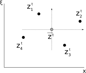
Figure 2. Phase space coordinates relative to the “center of mass”.

We have

(5.5) $$\begin{split}\frac{d}{dt}\overline{x^{t}}_{j}&=\overline{\xi^{t}}_{j}=O(\max_{j,k}|\xi_{j}^{t}-\xi_{k}^{t}|)=O\Bigl{(}|\xi_{j}-\xi_{k}|+\min\bigl{(}2^{\ell^{*}},\tfrac{2^{2\ell^{*}}}{\max|\xi_{j}-\xi_{k}|}\bigr{)}\Bigr{)}\\ \frac{d}{dt}\overline{\xi^{t}}_{j}&=\tfrac{1}{4}\sum_{k}\partial_{x}V(t,x^{t}_{k})-\partial_{x}V(t,x^{t}_{j})\\ &=\tfrac{1}{4}\sum_{k}(x^{t}_{k}-x^{t}_{j})\int_{0}^{1}\partial^{2}_{x}V(t,(1-\theta)x_{j}^{t}+\theta x_{k}^{t})\,d\theta\\ &=O(2^{\ell^{*}}).\end{split}$$

Note that

(5.6) $$\max_{j}|\overline{x^{t}}_{j}|\sim\max_{j,k}|x^{t}_{j}-x^{t}_{k}|,\quad\max_{j}|\overline{\xi^{t}}_{j}|\sim\max_{j,k}|\xi^{t}_{j}-\xi^{t}_{k}|.$$

Consider the operator

$$D=\partial_{t}+\overline{\xi^{t}}\partial_{x}.$$

We compute

$$\begin{split}-D\Phi&=\sum\sigma_{j}h(t,z_{j}^{t})+\sum\sigma_{j}[(x-x_{j}^{t})\partial_{x}V(t,x_{j}^{t})-\overline{\xi^{t}}\xi_{j}^{t}]\\ &=\tfrac{1}{2}\sum\sigma_{j}|\overline{\xi^{t}}_{j}|^{2}+\sum\sigma_{j}\bigl{[}V(t,x_{j}^{t})+(x-x_{j}^{t})\partial_{x}V(t,x_{j}^{t})\bigr{]}.\end{split}$$

This is more transparent when expressed in the relative variables $\overline{x^{t}}_{j}$ and $\overline{\xi^{t}}_{j}$. Each term in the second sum can be written as

$$V(t,\overline{x^{t}} +\overline{x^{t}}_{j})+(x-x_{j}^{t})\partial_{x}V(t,\overline{x^{t}}+\overline{x^{t}}_{j})$$

$$=V(t,\overline{x^{t}}+\overline{x^{t}}_{j})-V(t,\overline{x^{t}})-\overline{x^{t}}_{j}\partial_{x}V(t,\overline{x^{t}})+V(t,\overline{x^{t}})+\overline{x^{t}}_{j}\partial_{x}V(t,\overline{x^{t}})+(x-x_{j}^{t})\partial_{x}V(t,\overline{x^{t}})$$

$$\quad+(x-x_{j}^{t})(\partial_{x}V(t,\overline{x^{t}}+\overline{x^{t}}_{j})-\partial_{x}V(t,\overline{x^{t}}))$$

$$=V^{\overline{z}}(t,\overline{x^{t}}_{j})+V(t,\overline{x^{t}})+(x-x_{j}^{t})[\partial_{x}V^{\overline{z}}](t,\overline{x^{t}}_{j})+(x-\overline{x^{t}})\partial_{x}V(t,\overline{x^{t}}),$$

where

(5.7) $$V^{\overline{z}}(t,x)=V(t,\overline{x^{t}}+x)-V(t,\overline{x^{t}})-x\partial_{x}V(t,\overline{x^{t}})=x^{2}\int_{0}^{1}(1-s)\partial^{2}_{x}V(t,\overline{x^{t}}+sx)\,ds.$$

The terms without the subscript $j$ cancel upon summing, and we obtain

(5.8) $$-D\Phi=\tfrac{1}{2}\sum\sigma_{j}|\overline{\xi^{t}}_{j}|^{2}+\sum\sigma_{j}[V^{\bar{z}}(t,\overline{x^{t}}_{j})+(x-x_{j}^{t})[\partial_{x}V^{\overline{z}}](t,\overline{x^{t}}_{j})].$$

Therefore the contribution to $D\Phi$ from $V$ depends essentially only on the differences $x^{t}_{j}-x^{t}_{k}$. Invoking (5.1), (5.2), and (5.6), we see that the second sum is at most $O(2^{2\ell^{*}})$.

Note also that

$$(\overline{\xi^{t}}_{j})^{2}=(\overline{\xi}_{j})^{2}+O(2^{2\ell^{*}}),$$

as can be seen via (5.5), the fundamental theorem of calculus, and the time restriction (5.1). It follows that if

(5.9) $$\Bigl{|}\sum_{j}\sigma_{j}(\overline{\xi}_{j})^{2}\Bigr{|}\geq C\cdot 2^{2\ell^{*}}$$

for some large constant $C>0$, then on the support of the integrand

(5.10) $$\begin{split}|D\Phi|\gtrsim\Bigl{|}\sum_{j}\sigma_{j}(\overline{\xi}_{j})^{2}\Bigr{|}&=\tfrac{1}{2}\bigl{|}(\overline{\xi}_{1}+\overline{\xi}_{2})^{2}-(\overline{\xi}_{3}+\overline{\xi}_{4})^{2}+(\overline{\xi}_{1}-\overline{\xi}_{2})^{2}-(\overline{\xi}_{3}-\overline{\xi}_{4})^{2}\bigr{|}\\ &=\tfrac{1}{2}\bigl{|}|\xi_{1}-\xi_{2}|^{2}-|\xi_{3}-\xi_{4}|^{2}\bigr{|},\end{split}$$

where the last inequality follows from the fact that $\overline{\xi}_{1}+\overline{\xi}_{2}+\overline{\xi}_{3}+\overline{\xi}_{4}=0$.

The second derivative of the phase is

$$\begin{split}-D^{2}\Phi&=\sum\sigma_{j}\overline{\xi^{t}}_{j}\bigl{[}\tfrac{1}{4}\sum_{k}\partial_{x}V(t,x_{k}^{t})-\partial_{x}V(t,x_{j}^{t})\bigr{]}+\sum_{j}\sigma_{j}(x-x_{j}^{t})\xi_{j}^{t}\partial^{2}_{x}V(t,x_{j}^{t})\\ &\quad+\overline{\xi^{t}}\sum\sigma_{j}\partial_{x}V(t,x_{j}^{t})+\sum\sigma_{j}[\partial_{t}V(t,x_{j}^{t})+(x-x_{j}^{t})\partial_{t}\partial_{x}V(t,x_{j}^{t})]\\ &=\sum\sigma_{j}\overline{\xi^{t}}_{j}\bigl{[}\tfrac{1}{4}\sum_{k}\partial_{x}V(t,x_{k}^{t})-\partial_{x}V(t,x_{j}^{t})\bigr{]}+\sum\sigma_{j}(x-x_{j}^{t})\overline{\xi^{t}}_{j}\partial_{x}^{2}V(t,x_{j}^{t})\\ &\quad+\sum\sigma_{j}[\partial_{t}V(t,x_{j}^{t})+(x-x_{j}^{t})\partial_{t}\partial_{x}V(t,x_{j}^{t})]+\overline{\xi^{t}}\sum\sigma_{j}[\partial_{x}V(t,x_{j}^{t})+(x-x_{j}^{t})\partial^{2}_{x}V(t,x_{j}^{t})].\end{split}$$

We rewrite the last two sums as before to obtain

(5.11) $$\begin{split}-D^{2}\Phi&=\sum\sigma_{j}\overline{\xi^{t}}_{j}\bigl{[}\tfrac{1}{4}\sum_{k}\partial_{x}V(t,x_{k}^{t})-\partial_{x}V(t,x_{j}^{t})\bigr{]}+\sum\sigma_{j}(x-x_{j}^{t})\overline{\xi^{t}}_{j}\partial_{x}^{2}V(t,x_{j}^{t})\\ &\quad+\sum\sigma_{j}[(\partial_{t}V)^{\overline{z}}(t,\overline{x^{t}}_{j})+(x-x_{j}^{t})\partial_{x}(\partial_{t}V)^{\overline{z}}(t,\overline{x^{t}}_{j})]\\ &\quad+\overline{\xi^{t}}\sum\sigma_{j}[(\partial_{x}V)^{\overline{z}}(t,\overline{x^{t}}_{j})+(x-x_{j}^{t})\partial_{x}(\partial_{x}V)^{\overline{z}}(t,\overline{x^{t}}_{j})],\end{split}$$

where

$$\begin{split}(\partial_{t}V)^{\overline{z}}(t,x)&=x^{2}\int_{0}^{1}(1-s)\partial^{2}_{x}\partial_{t}V(t,\overline{x^{t}}+sx)\,ds\\ (\partial_{x}V)^{\overline{z}}(t,x)&=x^{2}\int_{0}^{1}(1-s)\partial^{3}_{x}V(t,\overline{x^{t}}+sx)\,ds.\end{split}$$

Assume that (5.9) holds. Write $e^{i\Phi}=\frac{D\Phi}{i|D\Phi|^{2}}\cdot De^{i\Phi}$ and integrate by parts to get

$$\begin{split}K^{\vec{\ell}}_{0}(\vec{z})&\lesssim\Bigl{|}\int e^{i\Phi}\frac{D^{2}\Phi}{(D\Phi)^{2}}\prod U_{j}\psi(x-x_{j}^{t})\theta_{\ell_{j}}(x-x_{j}^{t})\,\eta(t)dxdt\Bigr{|}\\ &+\Bigl{|}\int e^{i\Phi}\frac{1}{(D\Phi)}D\prod U_{j}\psi(x-x_{j}^{t})\theta_{\ell_{j}}(x-x_{j}^{t})\,\eta(t)dxdt\Bigr{|}\\ &\lesssim\Bigl{|}\int e^{i\Phi}\frac{D^{2}\Phi}{(D\Phi)^{2}}\prod U_{j}\psi(x-x_{j}^{t})\theta_{\ell_{j}}(x-x_{j}^{t})\,\eta(t)dxdt\Bigr{|}\\ &+\Bigl{|}\int e^{i\Phi}\frac{2D^{2}\Phi}{(D\Phi)^{3}}D\prod U_{j}\psi(x-x_{j}^{t})\theta_{\ell_{j}}(x-x_{j}^{t})\,\eta(t)dxdt\Bigr{|}\\ &+\Bigl{|}\int e^{i\Phi}\frac{1}{(D\Phi)^{2}}D^{2}\prod U_{j}\psi(x-x_{j}^{t})\theta_{\ell_{j}}(x-x_{j}^{t})\,\eta(t)dxdt\Bigr{|}\\ &=I+II+III.\end{split}$$

Note that after the first integration by parts, we only repeat the procedure for the second term. The point of this is to avoid higher derivatives of $\Phi$, which may be unacceptably large due to factors of $\overline{\xi^{t}}$.

Consider first the contribution from $I$. Write $I\leq I_{a}+I_{b}+I_{c}$, where $I_{a}$, $I_{b}$, $I_{c}$ correspond respectively to the first, second, and third lines in the expression (5.11) for $D^{2}\Phi$.

In view of (4.3), (5.2), (5.5), and (5.10), we have

$$\begin{split}I_{a}&\lesssim_{N}\int\frac{2^{\ell^{*}}\sum_{j}|\overline{\xi^{t}}_{j}|}{|D\Phi|^{2}}\prod_{j}2^{-\ell_{j}N}\chi\Bigl{(}\frac{x-x_{j}^{t}}{2^{\ell_{j}}}\Bigr{)}\,\eta(t)dxdt\\ &\lesssim_{N}\frac{2^{2\ell^{*}}(1+\sum|\overline{\xi}_{j}|)}{\bigl{|}(\xi_{1}-\xi_{2})^{2}-(\xi_{3}-\xi_{4})^{2}\bigr{|}^{2}}\cdot\int\prod_{j}2^{-\ell_{j}N}\chi\Bigl{(}\frac{x-x_{j}^{t}}{2^{\ell_{j}}}\Bigr{)}\,\eta(t)dxdt\\ &\lesssim_{N}2^{-\ell^{*}N}\cdot\frac{\langle\xi_{1}+\xi_{2}-\xi_{3}-\xi_{4}\rangle+|\xi_{1}-\xi_{2}|+|\xi_{3}-\xi_{4}|}{\bigl{|}(\xi_{1}-\xi_{2})^{2}-(\xi_{3}-\xi_{4})^{2}\bigr{|}^{2}}\cdot\frac{1}{1+|\xi_{1}-\xi_{2}|+|\xi_{3}-\xi_{4}|},\end{split}$$

where we have observed that

$$\begin{split}\sum_{j}|\overline{\xi}_{j}|&\sim\bigl{(}\sum_{j}|\overline{\xi}_{j}|^{2}\bigr{)}^{1/2}\sim\bigl{(}|\overline{\xi}_{1}+\overline{\xi}_{2}|^{2}+|\overline{\xi}_{1}-\overline{\xi}_{2}|^{2}+|\overline{\xi}_{3}+\overline{\xi}_{4}|^{2}+|\overline{\xi}_{3}-\overline{\xi}_{4}|^{2}\bigr{)}^{1/2}\\ &\lesssim|\xi_{1}+\xi_{2}-\xi_{3}-\xi_{4}|+|\xi_{1}-\xi_{2}|+|\xi_{3}-\xi_{4}|.\end{split}$$

Similarly,

$$\begin{split}I_{b}&\lesssim_{N}\int\frac{2^{2\ell^{*}}}{|D\Phi|^{2}}\prod_{j}2^{-\ell_{j}N}\chi\Bigl{(}\frac{x-x_{j}^{t}}{2^{\ell_{j}}}\Bigr{)}\,\eta(t)dxdt\\ &\lesssim_{N}\frac{2^{-\ell^{*}N}}{\bigl{|}(\xi_{1}-\xi_{2})^{2}-(\xi_{3}-\xi_{4})^{2}\bigr{|}^{2}}\cdot\frac{1}{1+|\xi_{1}-\xi_{2}|+|\xi_{3}-\xi_{4}|}.\end{split}$$

To estimate $I_{c}$, use the decay hypothesis $|\partial_{x}^{3}V|\lesssim\langle x\rangle^{-1-\varepsilon}$ to obtain

$$\begin{split}I_{c}&\lesssim_{N}\int\frac{2^{2\ell^{*}}|\overline{\xi^{t}}|}{|D\Phi|^{2}}\Bigl{(}\int_{0}^{1}\sum_{j}\langle\overline{x^{t}}+s\overline{x^{t}}_{j}\rangle^{-1-\varepsilon}\,ds\Bigr{)}\prod_{j}2^{-\ell_{j}N}\chi\Bigl{(}\frac{x-x_{j}^{t}}{2^{\ell_{j}}}\Bigr{)}\,\eta(t)dxdt\\ &\lesssim_{N}\frac{2^{-\ell^{*}N}}{|(\xi_{1}-\xi_{2})^{2}-(\xi_{3}-\xi_{4})^{2}|^{2}}\int_{0}^{1}\sum_{j}\int_{|t|\leq\delta_{0}}|\overline{\xi^{t}}|\langle\overline{x^{t}}+s\overline{x^{t}}_{j}\rangle^{-1-\varepsilon}\,dtds.\end{split}$$

The integral on the right is estimated in the following technical lemma.

Lemma 5.1.

$$\int_{0}^{1}\sum_{j}\int_{|t|\leq\delta_{0}}|\overline{\xi^{t}}|\langle\overline{x^{t}}+s\overline{x^{t}}_{j}\rangle^{-1-\varepsilon}\,dtds=O(2^{(2+\varepsilon)\ell^{*}}).$$

Proof.

It will be convenient to replace the average bicharacteristic $(\overline{x^{t}},\overline{\xi^{t}})$ with the ray $(\overline{x}^{t},\overline{\xi}^{t})$ starting from the average initial data. We claim that

$$|\overline{x^{t}}-\overline{x}^{t}|+|\overline{\xi^{t}}-\overline{\xi}^{t}|=O(2^{\ell^{*}})$$

during the relevant $t$, for Hamilton’s equations imply that

$$\begin{split}\overline{x^{t}}-\overline{x}^{t}&=-\int_{0}^{t}(t-\tau)\Bigl{(}\frac{1}{4}\sum_{k}\partial_{x}V(\tau,x_{k}^{\tau})-\partial_{x}V(\tau,\overline{x}^{\tau})\Bigr{)}\,d\tau\\ &=-\int_{0}^{t}(t-\tau)\Bigl{(}\frac{1}{4}\sum_{k}(\overline{x^{\tau}}_{k}+\overline{x^{\tau}}-\overline{x}^{\tau})\int_{0}^{1}\partial^{2}_{x}V(\tau,\overline{x}^{\tau}+s(x_{k}^{\tau}-\overline{x}^{\tau}))\,ds\Bigr{)}\,d\tau\\ &=-\int_{0}^{t}(t-\tau)(\overline{x^{\tau}}-\overline{x}^{\tau})\Bigl{[}\int_{0}^{1}\frac{1}{4}\sum_{k}\partial^{2}_{x}V(\tau,\overline{x}^{\tau}+s(x_{k}^{\tau}-\overline{x}^{\tau}))\,ds\Bigr{]}\,d\tau+O(2^{\ell^{*}}t^{2}),\end{split}$$

and we can invoke Gronwall. Similar considerations yield the bound for $|\overline{\xi^{t}}-\overline{\xi}^{t}|$. As also $\overline{x^{t}}_{j}=O(2^{\ell^{*}})$, we are reduced to showing

(5.12) $$\int_{|t|\leq\delta_{0}}|\overline{\xi}^{t}|\langle\overline{x}^{t}\rangle^{-1-\varepsilon}\,dt=O(1).$$

Integrating the ODE

$$\tfrac{d}{dt}\overline{x}^{t}=\overline{\xi}^{t}\quad\text{and}\quad\tfrac{d}{dt}\overline{\xi}^{t}=-\partial_{x}V(t,\overline{x}^{t})$$

yields the estimates

$$\begin{split}|\overline{x}^{t}-\overline{x}^{s}-(t-s)\overline{\xi}^{s}|&\leq C|t-s|^{2}(|\overline{x}^{s}|+|(t-s)\overline{\xi}^{s}|)\\ |\overline{\xi}^{t}-\bar{\xi}^{s}|&\leq C|t-s|(|\overline{x}^{s}|+|(t-s)\overline{\xi}^{s}|)\end{split}$$

for some constant $C$ depending on $\|\partial_{x}^{2}V\|_{L^{\infty}}$. By subdividing the time interval $[-\delta_{0},\delta_{0}]$ if necessary, we may assume in (5.12) that $(1+C)|t|\leq 1/10$.

Consider separately the cases $|\overline{x}|\leq|\overline{\xi}|$ and $|\overline{x}|\geq|\overline{\xi}|$. When $|\overline{x}|\leq|\overline{\xi}|$ we have

$$2|\overline{\xi}|\geq|\overline{\xi}^{t}|\geq|\overline{\xi}|-\tfrac{1}{5}|\overline{\xi}|\geq\tfrac{1}{2}|\overline{\xi}|$$

(assuming, as we may, that $|\overline{\xi}|\geq 1$) and the bound (5.12) follows from the change of variables $y=\bar{x}^{t}$. If instead $|\overline{x}|\geq|\overline{\xi}|$, then $|\overline{x}^{t}|\geq\tfrac{1}{2}|\overline{x}|$ and $|\overline{\xi}^{t}|\leq 2|\overline{x}|$, which also yields the desired bound. ∎

Returning to $I_{c}$, we conclude that

$$I_{c}\lesssim_{N}\frac{2^{-\ell^{*}N}}{|(\xi_{1}-\xi_{2})^{2}-(\xi_{3}-\xi_{4})^{2}|^{2}}.$$

Overall,

$$\begin{split}I&\leq I_{a}+I_{b}+I_{c}\lesssim_{N}2^{-\ell^{*}N}\frac{\langle\xi_{1}+\xi_{2}-\xi_{3}-\xi_{4}\rangle}{|(\xi_{1}-\xi_{2})^{2}-(\xi_{3}-\xi_{4})^{2}|^{2}}.\end{split}$$

For $II$, we have

(5.13) $$D[U_{j}\psi(x-x_{j}^{t})]=-iH_{j}U_{j}\psi(x-x_{j}^{t})-\overline{\xi^{t}}_{j}\partial_{x}U_{j}\psi(x-x_{j}^{t})$$

and estimating as for $I$ we get

$$\begin{split}II&\lesssim_{N}\frac{1+\sum_{j}|\overline{\xi}_{j}|}{|(\xi_{1}-\xi_{2})^{2}-(\xi_{3}-\xi_{4})^{2}|}\int\frac{|D^{2}\Phi|}{|D\Phi|^{2}}\prod 2^{-\ell_{j}N}\chi\Bigl{(}\frac{x-x_{j}^{t}}{2^{\ell_{j}}}\Bigr{)}\,\eta dxdt\\ &\lesssim_{N}2^{-\ell^{*}N}\Bigl{(}\frac{\langle\xi_{1}+\xi_{2}-\xi_{3}-\xi_{4}\rangle+|\xi_{1}-\xi_{2}|+|\xi_{3}-\xi_{4}|}{|(\xi_{1}-\xi_{2})^{2}-(\xi_{3}-\xi_{4})^{2}|}\Bigr{)}\frac{\langle\xi_{1}+\xi_{2}-\xi_{3}-\xi_{4}\rangle}{|(\xi_{1}-\xi_{2})^{2}-(\xi_{3}-\xi_{4})^{2}|^{2}}.\end{split}$$

It remains to consider $III$. The derivatives can distribute in various ways:

(5.14) $$\begin{split}III&\lesssim\frac{1}{|(\xi_{1}-\xi_{2})^{2}-(\xi_{3}-\xi_{4})^{2}|^{2}}\Bigl{\{}\int|D^{2}[U_{1}\psi(x-x_{1}^{t})]\prod_{j=2}^{4}U_{j}\psi(x-x^{t}_{j})\prod_{k=1}^{4}\theta_{\ell_{k}}(x-x_{k}^{t})\eta|\,dxdt\\ &\quad+\int\Bigl{|}D[U_{1}\psi(x-x_{1}^{t})]D[U_{2}\psi(x-x_{2}^{t})]\prod_{j=3}^{4}U_{j}\psi(x-x^{t}_{j})\prod_{k=1}^{4}\theta_{\ell_{k}}(x-x_{k}^{t})\eta\Bigr{|}\,dxdt\\ &\quad+\int\Bigl{|}D\prod_{j}U_{j}\psi(x-x^{t}_{j})D\prod_{k}\theta_{\ell_{k}}(x-x_{k}^{t})\eta\Bigr{|}\,dxdt\\ &\quad+\int\Bigl{|}\prod_{j}U_{j}\psi(x-x^{t}_{j})D^{2}\prod_{k}\theta_{\ell_{k}}(x-x_{k}^{t})\eta\Bigr{|}\,dxdt\Bigr{\}},\end{split}$$

where the first two terms represent sums over the appropriate permutations of indices.

We focus on the terms involving double derivatives of $U_{j}$ as the other terms can be dealt with as in the estimate for $II$. From (5.13),

(5.15) $$\begin{split}D^{2}[U_{j}\psi(x-x_{j}^{t})]&=-i\partial_{t}V_{j}(t,x-x_{j}^{t})U_{j}\psi(x-x_{j}^{t})-(H_{j})^{2}U_{j}\psi(x-x_{j}^{t})\\ &+2i\overline{\xi^{t}}_{j}\partial_{x}H_{j}U_{j}\psi(x-x_{j}^{t})-\Bigl{[}\tfrac{1}{4}\sum_{k}\partial_{x}V(t,x_{k}^{t})-\partial_{x}V(t,x_{j}^{t})\Bigr{]}\partial_{x}U_{j}\psi(x-x_{j}^{t})\\ &+(\overline{\xi^{t}}_{j})^{2}\partial^{2}_{x}U_{j}\psi(x-x_{j}^{t}).\end{split}$$

Recalling from (4.2) that

$$\partial_{t}V_{j}(t,x)=x^{2}\Bigl{[}\xi_{j}^{t}\int_{0}^{1}(1-s)\partial_{x}^{3}V(t,x_{j}^{t}+sx)ds+\int_{0}^{1}(1-s)\partial_{t}\partial^{2}_{x}V(t,x_{j}^{t}+sx)\,ds\Bigr{]},$$

it follows that

$$\begin{split}\int\Bigl{|}\partial_{t}V_{1}(t,x-x_{1}^{t})&U_{1}\psi(x-x_{1}^{t})\prod_{j=2}^{4}U_{j}\psi(x-x_{j}^{t})\prod_{k=1}^{4}\theta_{\ell_{k}}(x-x_{k}^{t})\Bigr{|}\,\eta(t)dxdt\\ &\lesssim 2^{2\ell_{1}}\int\Bigl{[}\int_{0}^{1}|\xi_{1}^{t}\partial^{3}V_{x}(t,x_{1}^{t}+s(x-x_{1}^{t}))|\,ds\\ &\quad+\int_{0}^{1}|\partial_{t}\partial^{2}_{x}V(t,x_{j}^{t}+s(x-x_{j}^{t}))\,ds\Bigr{]}\prod_{j}2^{-\ell_{j}N}\chi\Bigl{(}\frac{x-x_{j}^{t}}{2^{\ell_{j}}}\Bigr{)}\,\eta dxdt\\ &\lesssim_{N}2^{-\ell^{*}N},\end{split}$$

where the terms involving $\partial^{3}_{x}V$ are handled as in $I_{c}$ above. Also, from (4.3) and (5.2),

$$\begin{split}&\int\Bigl{|}(\overline{\xi}_{1}^{t})^{2}\partial_{x}^{2}U_{1}\psi(x-x_{1}^{t})\prod_{j=2}^{4}U_{j}\psi(x-x_{j}^{t})\prod_{k=1}^{4}\theta_{\ell_{k}}(x-x_{k}^{t})\Bigr{|}\,\eta(t)dxdt\lesssim_{N}\frac{2^{-\ell^{*}N}(1+|\overline{\xi}_{1}|^{2})}{1+|\xi_{1}-\xi_{2}|+|\xi_{3}-\xi_{4}|}.\end{split}$$

The intermediate terms in (5.15) and the other terms in the the expansion (5.14) yield similar upper bounds. We conclude overall that

$$\begin{split}III&\lesssim_{N}2^{-\ell^{*}N}\Bigl{(}\frac{1}{|(\xi_{1}-\xi_{2})^{2}-(\xi_{3}-\xi_{4})^{2}|^{2}}+\frac{(1+\sum_{j}|\overline{\xi}_{j}|)^{2}}{|(\xi_{1}-\xi_{2})^{2}-(\xi_{3}-\xi_{4})^{2}|^{2}\cdot(1+|\xi_{1}-\xi_{2}|+|\xi_{3}-\xi_{4}|)}\Bigr{)}\\ &\lesssim_{N}2^{-\ell^{*}N}\Bigl{(}\frac{1}{|(\xi_{1}-\xi_{2})^{2}-(\xi_{3}-\xi_{4})^{2}|^{2}}+\frac{\langle\xi_{1}+\xi_{2}-\xi_{3}-\xi_{4}\rangle^{2}+(|\xi_{1}-\xi_{2}|+|\xi_{3}-\xi_{4}|)^{2}}{\bigl{|}|\xi_{1}-\xi_{2}|^{2}-|\xi_{3}-\xi_{4}|^{2}\bigr{|}^{2}\cdot(1+|\xi_{1}-\xi_{2}|+|\xi_{3}-\xi_{4}|)}\Bigr{)}\\ &\lesssim_{N}2^{-\ell^{*}N}\frac{\langle\xi_{1}+\xi_{2}-\xi_{3}-\xi_{4}\rangle^{2}+|\xi_{1}-\xi_{2}|+|\xi_{3}-\xi_{4}|}{|(\xi_{1}-\xi_{2})^{2}-(\xi_{3}-\xi_{4})^{2}|^{2}}.\end{split}$$

Note also that in each of the integrals $I$, $II$, and $III$ we may integrate by parts in $x$ to obtain arbitrarily many factors of $|\xi_{1}+\xi_{2}-\xi_{3}-\xi_{4}|^{-1}$. All instances of $\langle\xi_{1}+\xi_{2}-\xi_{3}-\xi_{4}\rangle$ in the above estimates may therefore be replaced by $1$.

Combining $I$, $II$, and $III$, under the hypothesis (5.9) we obtain

$$\begin{split}|K^{\vec{\ell}}_{0}(\vec{z})|\lesssim_{N}2^{-\ell^{*}N}\frac{1+|\xi_{1}-\xi_{2}|+|\xi_{3}-\xi_{4}|}{\bigl{|}(\xi_{1}-\xi_{2})^{2}-(\xi_{3}-\xi_{4})^{2}\bigr{|}^{2}}.\end{split}$$

Combining this with (5.4), we get

(5.16) $$\begin{split}|K^{\vec{\ell}}_{0}(\vec{z})|&\lesssim_{N_{1},N_{2}}2^{-\ell^{*}N_{1}}\min\Bigl{(}\frac{\langle\xi_{1}+\xi_{2}-\xi_{3}-\xi_{4}\rangle^{-N_{2}}}{1+|\xi_{1}-\xi_{2}|+|\xi_{3}-\xi_{4}|},\frac{1+|\xi_{1}-\xi_{2}|+|\xi_{3}-\xi_{4}|}{\bigl{|}(\xi_{1}-\xi_{2})^{2}-(\xi_{3}-\xi_{4})^{2}\bigr{|}^{2}}\Bigr{)}\end{split}$$

for any $N_{1},N_{2}>0$. Lemma 4.4 now follows from summing in $\vec{\ell}$.