Deterministic global optimization using space-filling curves and multiple estimates of Lipschitz and Hölder constants
Abstract
In this paper, the global optimization problem with being a hyperinterval in and satisfying the Lipschitz condition with an unknown Lipschitz constant is considered. It is supposed that the function can be multiextremal, non-differentiable, and given as a ‘black-box’. To attack the problem, a new global optimization algorithm based on the following two ideas is proposed and studied both theoretically and numerically. First, the new algorithm uses numerical approximations to space-filling curves to reduce the original Lipschitz multi-dimensional problem to a univariate one satisfying the Hölder condition. Second, the algorithm at each iteration applies a new geometric technique working with a number of possible Hölder constants chosen from a set of values varying from zero to infinity showing so that ideas introduced in a popular DIRECT method can be used in the Hölder global optimization. Convergence conditions of the resulting deterministic global optimization method are established. Numerical experiments carried out on several hundreds of test functions show quite a promising performance of the new algorithm in comparison with its direct competitors.
Key Words. Global optimization, Lipschitz functions, space-filling curves, Hölder functions, deterministic numerical algorithms, DIRECT, classes of test functions.
1 Introduction
Let us consider the following global optimization problem
| (1.1) |
where is a hyperinterval in . It is supposed that the objective function can be multiextremal, possibly non-differentiable and it satisfies the Lipschitz condition
| (1.2) |
with an unknown constant , in the Euclidean norm. This statement can very frequently be met in applications where each evaluation of can be very expensive from the computational point of view (see, e.g., [3, 5, 10, 19, 28, 35, 40, 42], etc.). Due to this reason, in the literature there exist numerous methods dedicated to the problem (1.1), (1.2) (together with references indicated above we can mention such recent publications as [2, 4, 5, 17, 18, 26, 27, 43, 44]). It should be also mentioned that methods for problems where the gradient of the objective function satisfies the Lipschitz condition were also studied (see, e.g., [4, 13, 20, 24, 34, 35, 37], etc.).
One of the main issues regarding the problem (1.1), (1.2) is related to the treatment of the Lipschitz constant . In the literature, there exist several approaches for acquiring the Lipschitz information that can be distinguished with respect to the way the Lipschitz constant is estimated during the process of optimization. For instance, there exist algorithms (see, e.g., [4, 10, 11, 27, 29]) that use an a priori given estimate of (it should be mentioned that usually in practice it is difficult to obtain valid estimates) or an adaptive estimate that is recalculated at each iteration of the method (see, e.g., [28, 37, 38, 40]).
It is well known that estimates of the Lipschitz constant have a significant influence on the convergence and the speed of the global optimization algorithms (see [37, 38, 40]). Namely, tight estimates can accelerate the search, overestimates can slow it down, and underestimates can lead to losing the global solution. Algorithms that use in their work a global estimate or an a priori given estimate do not take into account any local information about the behavior of the objective function over small subregions of the domain . It has been shown in [16, 21, 25, 32, 34, 38, 40] that a smart usage of local estimates of the local Lipschitz constants over subregions allows one to significantly accelerate the global search. Naturally, a balancing between the local and global information must be performed in an appropriate way in order to avoid missing the global solution. Another interesting approach that has been introduced in [15] uses at each iteration several estimates of the Lipschitz constant . This algorithm works by partioning the hyperinterval in subintervals (called hereinafter also subboxes) and due to this reason it has been called by its authors DIRECT (DIviding RECTangles).
We can see therefore that in the literature there exist four practical strategies to obtain a Lipschitz information for its subsequent usage in numerical methods: a) to consider the real constant , if it is given, or to use its overestimate when it is possible; b) to calculate dynamically a global a global (i.e., the same for the whole search region) adaptive estimate of ; c) to consider estimates of local Lipschitz constants related to subintervals of the search region ; d) to take into consideration a set of estimates of selected among all possible values varying from zero to infinity. In this paper, our attention will be dedicated to this fourth alternative.
As was mentioned above, in the literature there exists a variety of numerical methods dedicated to the problem (1.1), (1.2). One of non trivial views on the problem consists of the reduction of the dimension of (1.1), (1.2) with the help of space-filling curves. These curves, first introduced by Peano (1890) and Hilbert (1891) (see [1, 31, 38, 39, 40, 41]), emerge as the limit objects generated by an iterative process. They are fractals constructed using the principle of self-similarity. Peano-Hilbert curves fill in the hypercube , i.e., they pass through every point of , and this gave rise to the term space-filling curves. Examples of construction of these curves in two dimensions are given in Fig. 1.
It has been shown (see [1],[39],[40]) that, by using space filling curves, the multidimensional global minimization problem (1.1), (1.2) can be turned into a one-dimensional problem. In particular, Strongin has proved in [39] that finding the global minimum of the Lipschitz function over a hypercube is equivalent to determining the global minimum of the function in an interval, i.e., it follows
| (1.3) |
where is the Peano curve. Moreover, the Hölder condition
| (1.4) |
holds (see [40]) for the function with the constant
| (1.5) |
where is the Lipschitz constant of the original multidimensional function from (1.1), (1.2).
Thus, one can try to solve the problem (1.1), (1.2) by using algorithms proposed for minimizing Hölderian functions (1.3), (1.4) in one dimension. To do this in practice, three main steps should be executed if one wishes to use methods that partition the search region and try to obtain and to use a Lipschitz/Hölder information (see [28, 33, 37] for a general description of this kind of methods, their convergence properties, etc.). First, in order to realize the passage from the multi-dimensional problem to the one-dimensional one, computable approximations to the Peano curve should be employed in the numerical algorithms. Second, the Hölder constant from (1.4) should be estimated. Finally, a partition strategy of the search region should be chosen.
We have already seen above that in the Lipschitz global optimization there exist at least four ways to obtain estimates of the Lipschitz constant. When we move to the Hölder global optimization the situation is different. In the literature (see [12, 21, 22, 23, 24, 38]), there exist methods that use strategies a), b), and c) discussed above. However, inventing for the Hölder global optimization a strategy similar to the technique d) was an open problem since 1993 when the article [15] showing how to use simultaneously several estimates of has been published. In this paper, we close this gap and propose an algorithm that uses several estimates of the Hölder constant at each iteration employing space-filling curves, central point based partition strategies, and Hölderian minorants.
The rest of the paper has the following structure. In Section 2, difficulties regarding the usage of the strategy d) in the Hölderian framework and the proposed solution are presented. In Section 3, a new algorithm for solving the problem (1.1), (1.2) and its convergence properties are described. The new method uses numerical approximations to Peano space-filling curves and the scheme of representation of intervals with Hölderian minorants from Section 2. Section 4 presents results of numerical experiments that compare the new method with its competitors on 800 test functions randomly generated by the GKLS-generator from [9]. Finally, Section 5 contains a brief conclusion.
2 Lipschitz and Hölder minorants in one dimension
Let us consider a one-dimensional function satisfying the Lipschitz condition with a constant over the interval . Then it follows from the Lipschitz condition that
| (2.1) |
| (2.2) |
where is (see Fig. 2, left) a piece-wise linear discontinuous minorant (called often also support function) for over each subinterval , and
| (2.3) |
The values , called characteristics and being lower bounds for the function over each interval , can easily be calculated. In fact, if we suppose that an overestimate of the Lipschitz constant is given, then it follows
| (2.4) |
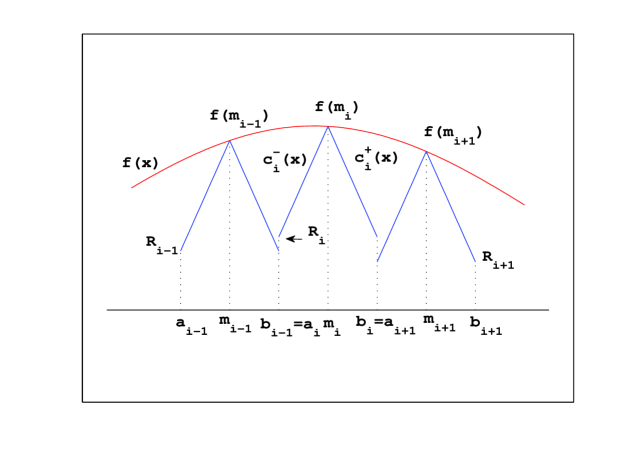
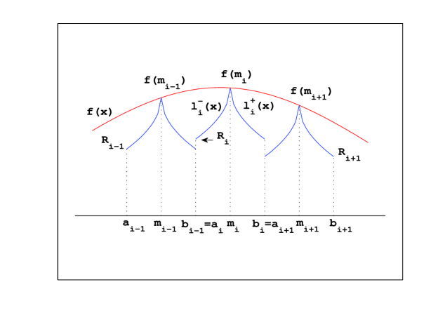
However, in order to solve the multidimensional problem (1.1), (1.2) by using space-filling curves, instead of working with Lipschitz functions, we should focus our attention on the one-dimensional Hölderian function from (1.3). It follows from (1.4) that, for all we have
| (2.5) |
If a point is fixed, then the function
is a minorant for over . Then, analogously to (2.1)–(2.3), we obtain that the function
| (2.6) |
| (2.7) |
is a discontinuous nonlinear minorant for (see Fig. 2, right). The values , are lower bounds for the function over each interval , and can be calculated as follows if an overestimate of the Hölder constant is given
| (2.8) |
As it was discussed above, the DIRECT algorithm works simultaneously with several estimates of the Lipschitz constant at each iteration. One of the key features that allow it to do this is a smart representation of intervals , in the two-dimensional diagram shown in Fig. 3. In this Figure, we have intervals , , , , and that are represented by the dots , , , , and , respectively. The horizontal coordinate of each dot is equal to , i.e., half of the length of the respective interval , and the vertical coordinate is equal to where is from (2.3) (see, e.g., the dot and its coordinates). Let us consider now the intersection of the vertical coordinate axis with the line having the slope and passing through each dot representing subintervals in the diagram shown in Fig. 3. It is possible to see that this intersection gives us exactly the characteristic from (2.4), i.e., the lower bound for over the corresponding subinterval if (note that the points on the vertical axis () do not represent any subinterval).
It can immediately be seen that the diagram allows one to determine very easily an interval with the minimal characteristic (in Fig. 3 this interval is represented by the dot , its characteristic is ). In the Lipschitz global optimization (see, e.g., [28, 33, 37, 38, 40]), the operation of finding an interval with the minimal characteristic (that can be calculated in different ways in different algorithms) is an important one. It is executed at each iteration, the found interval is then subdivided and is evaluated at new points belonging to this interval. Moreover, since we do not know the exact value of the real Lipschitz constant , the scheme presented in Fig. 3 allows one (see [15]) to take into consideration all possible values of from zero to infinity111In fact, it is easy to see that if we connect the points and by a line and indicate its slope by then for all constants the interval will have the minimal characteristic and, therefore it should be subdivided. Analogously, for all constants the interval will have the minimal characteristic. Then, if we subdivide both intervals, and , then the interval corresponding to the real constant will be subdivided even though we are not know this value . Thus, the diagram really allows one to consider all possible values of the Lipschitz constant from zero to infinity and to choose a small group of intervals for the subsequent subdivision ensuring that the interval corresponding to the correct Lipschitz constant belongs to this group. and to choose a set of promising intervals for partitioning (this issue will be discussed in detail later).
Let us try now to construct a similar diagram in the framework of the Hölder optimization where the nonlinear support functions from (2.7) shown in Fig. 2, right, are built over each subinterval. In Fig. 4, intervals , , , , and are again represented by dots , , , , and , respectively. If we take an estimate of the Hölder constant , then characteristic of the interval represented by the dot is given by the vertical coordinate of the intersection point of the auxiliary curve (2.7) passed through the point and the vertical coordinate axis.
We can see in Fig. 4 that the curves constructed using the estimate and representing the nonlinear support function (2.7) can intersect each other in different ways. The procedure of the selection of subintervals for producing new trials (trial is an evaluation of at a point that is called trial point) is based on estimates of the lower bounds of the objective function over current subboxes. Subintervals for the further subdivision are chosen taking into account all possible values of the Hölder constant . Due to numerous possible intersections of the curves at the representation shown in Fig. 4, it becomes unclear how to select, for all possible values of , the set of promising intervals that must be partitioned at each iteration .
This difficulty that seemed unsolvable since 1993 did not allow people to construct global optimization algorithms working in the framework of the Hölder global optimization with all possible Hölder constants. This problem is solved in the next section that proposes an algorithm that uses, on the one hand, Peano space-filling curves to reduce the multi-dimensional problem (1.1), (1.2) to one dimension and, on the other hand, multiple estimates of the Hölder (Lipschitz) constant. The algorithm for solving one-dimensional Hölder global optimization problems in the spirit of the DIRECT method is a part of it.
3 The new algorithm
In order to construct a procedure allowing one to select, at each iteration of the algorithm, a set of intervals to be partitioned with respect to all possible values of the constant we proceed as follows. First, we introduce a new graphical representation of subintervals by using instead of Euclidean metric the Hölderian one. Namely, we propose to represent each interval by a dot with coordinates , where is the current partition of the one-dimensional search interval during the th iteration and coordinates of the point are calculated as follows
| (3.1) |
| (3.2) |
where is from (2.3), i.e., is the central point of the interval .
The introduction of the Hölderian metric allows us (see Fig. 5) to avoid the non-linearity and the intersection of minorants giving as a result a diagram similar to that from Fig. 3. In Fig. 5 we can see the representation of the same intervals considered in Fig. 4. Notice that in Fig. 5 the values in the horizontal axis are calculated in the Hölderian metric, while the vertical axis values coincide with those of Fig. 4. In this new representation, the intersection of the line with the slope passing through any dot representing an interval in the diagram of Fig. 5 and the vertical coordinate axis gives us exactly the characteristic (2.8) of the corresponding interval.
We can proceed now with the development of the new one-dimensional global optimization method following the spirit of the DIRECT algorithm and keeping in mind that we deal with the Hölderian metric. Each subinterval of a current partition is characterized by a lower bound of the objective function over . An interval is selected for a further partitioning if for some value of the possible Hölder constant it has the smallest lower bound for with respect to the other intervals present at this iteration. By changing the value of from zero to infinity, at each iteration , we select a set of intervals that will be partitioned.
Let us consider how this set of intervals is chosen during each iteration . The following definitions state a relation of domination between every two subintervals of the current partition of .
Definition 3.1
Given an estimate of the Hölder constant from (1.4), an interval dominates the interval with respect to if
Definition 3.2
An interval is said to be nondominated with respect to if for the chosen value there is no other interval in which dominates .
In order to be sure to subdivide the nondominated interval corresponding to the real constant , we can select the set of nondominated intervals with respect to all possible estimates . By using the new graphical representation shown in Fig. 5 it is easy to determine whether an interval dominates, with respect to an estimate of the Hölder constant , some other interval from the partition . For example, in Fig. 5 we can see that for the estimate we have
so, the interval dominates both intervals and with respect to . Furthermore, , i.e., the interval dominates the interval . Finally, the characteristic is the smallest one, and the interval dominates all others intervals with respect to , i.e., it is nondominated with respect to (see Fig. 5).
If a different value of the Hölder constant is considered (see Fig. 5), the interval still dominates the interval with respect to , because , but is dominated by the interval , since . Moreover, we have that , thus, for the chosen estimate the unique nondominated interval is . As we can see from this example, some intervals (, , and in Fig. 5) are always dominated by other intervals, independently on the chosen estimate of the Hölder constant. Other intervals ( and in Fig. 5) can be nondominated for one value and dominated for another one. The following definition will be very useful hereinafter.
Definition 3.3
An interval is called nondominated if there exists an estimate of the Hölder constant such that is nondominated with respect to .
In other words, nondominated intervals are intervals over which the objective function has the smallest lower bound from (2.8) for some particular estimate of the Hölder constant . Note that in the two-dimensional diagram , where and are from (3.1), (3.2), the nondominated intervals are located at the bottom of each group of points with the same horizontal coordinate. For example in Fig. 6 these points are designated as , , , , , , and . Not all of these intervals are nondominated: in fact, in Figure 6 the interval is dominated either by the interval (for example, with respect to , where corresponds to the slope of the line passed through the points and ), or by the interval (with respect to ). The interval is dominated by and , with respect to any positive estimate of the constant . The interval is dominated by . In Figure 6, dots , , , and represent nondominated intervals. The following theorem allow us to easily identify the set of nondominated intervals.
Theorem 3.1
In practice, nondominated intervals can be found by applying algorithms for identifying the convex hull of the dots (see, e.g., the algorithm called Jarvis march, or gift wrapping, see [30]).
We describe now the partition strategy adopted by the new algorithm for dividing subintervals in order to produce new trial points. When, at the generic iteration , we identify the set of nondominated intervals, we proceed with the subdivision of each of these intervals only if a significant improvement on the function values with respect to the current minimal value is expected. Once an interval becomes nondominated, it can be subdivided only if the following condition is satisfied:
| (3.3) |
where the lower bound is from (2.8). This condition prevents the algorithm from subdividing already well-explored small subintervals.
Let us suppose now that at the current iteration of the new algorithm a subinterval , represented in the two-dimensional diagram of Fig. 6 by the dot from (3.1), (3.2), has been chosen for partitioning. The subdivision of this interval is performed in such a way that three new equal subintervals of the length are created, i.e.,
| (3.4) |
| (3.5) |
The interval is removed from the two-dimensional diagram representing the current partition of the search interval, and the three newly generated subintervals are introduced both into and the diagram. Finally, two new trials and are performed at the points and of the intervals and , respectively, i.e.,
| (3.6) |
The central interval inherits the point at which the objective function has been evaluated when the original interval has been created.
Until now we have described the strategies assuming to work with a function in one dimension. As was stated above, Strongin has shown that multidimensional optimization problems can be solved by using modified algorithms proposed for minimizing functions in one dimension, and therefore in order to solve the global optimization problem in dimensions (1.1), (1.2) we can use the above developed one-dimensional global optimization method together with the space-filling curves. For an effective use of the Peano curve in our algorithm we need computable approximations of the curve (see [38, 40] for a detailed discussion and a code allowing one to implement such approximations). Hereinafter we denote by the approximation of level of the Peano curve. In Fig. 1 we can see examples of Peano curve approximations of the levels in dimension .
Suppose now that a global optimization method uses an approximation of the Peano curve to solve the multidimensional problem and provides a lower bound for the corresponding one-dimensional function . Then the value will be a lower bound for the function in dimension only along the curve . The following theorem establishes a lower bound for the function over the entire multidimensional search region given the value .
Theorem 3.2
Let be a lower bound along the space-filling curve for a multidimensional function , , satisfying Lipschitz condition with constant , i.e.,
Then the value
is a lower bound for over the entire region .
By using the space-filling curves we are able to work with a one-dimensional function in the interval . The level of the approximation of the Peano curve , is crucial for a good performance of the method. If is too small, the domain in dimensions may not be well “filled” and we risk losing the global solution. When grows, the reduced function in one dimension becomes more and more oscillating and the number of local minima increases when increases (see [23] for a detailed discussion on this topic). Then, due to the facts that we are in and that we use the metric of Hölder, it happens that the width of the nondominated interval to be partitioned at a generic iteration can become very small. When the dimension increases, the width of the subintervals can reach the computer precision. In order to avoid this situation another condition in addition to (3.3) is required. Namely, when an interval becomes nondominated, it can be subdivided only if the following condition is satisfied:
| (3.7) |
where is a parameter of the method.
Now, let us present the new algorithm called (ultidimensional lobal optimization lgorithm working with a et of estimates of the Hölder constant).
Algorithm MGAS
- Step 0.
-
(Initialization). Set the current iteration number .
Split the initial interval in three equal parts and set , , and compute the values of the function , , where is the -approximation of the Peano curve.
Set the current partition of the search interval .
Set the current number of intervals and the current number of trials .
Set , and .
After executing iterations, the iteration consists of the following steps.
- Step 1.
- Step 2.
-
(Subdivision of nondominated intervals) Set , and perform the following Steps 2.1-2.3:
- Step 2.1
(Interval selection). Select a new interval from such that
- Step 2.2
(Subdivision and sampling). Subdivide interval in three new equal subintervals, named , , , of the length , following (3.4), (3.5), and produce two new trial points accordingly to (3.6).
Eliminate the interval from , i.e., set , and update with the insertion of the three new intervals, i.e.,Increase both the current number of intervals , and the current number of trials .
Update the current record and the current record point if necessary. Step 2.3 (Next interval). Eliminate the interval from , i.e., set and . If , then go to Step 2.1. Otherwise go to Step 3. - Step 2.1
- Step 3.
-
(End of the current iteration). Increase the iteration counter . Go to Step 1 and start the next iteration.
Different stopping criteria can be used in the algorithm introduced above. One of them will be introduced in the next section presenting numerical experiments.
We proceed now to the study of convergence properties of the algorithm. Theorem 3.2 linking the multidimensional global optimization problem (1.1), (1.2) to the one-dimensional problem (1.3), (1.4) allows us to concentrate our attention on the convergence properties of the one-dimensional method. We shall study properties of an infinite sequence of trial points generated by the algorithm MGAS when we suppose that the number of iteration goes to infinity (i.e., in this case the algorithm does not stop). The following theorem establishes the so-called everywhere dense convergence of the method, i.e., convergence of the infinite sequence of trial points to any point of the one-dimensional search domain.
Theorem 3.3
If in (3.7), then for any point and any there exist an iteration number and a point , , such that .
Proof. The interval partition scheme (3.4), (3.5) used for each subdivision of intervals produces three new subintervals of the length equal to a third of the length of the subdivided interval. Since , to prove the Theorem it is sufficient to prove that for a fixed value , after a finite number of iterations , the largest subinterval of the current partition of the domain will have the length smaller than . In such a case, in the -neighborhood of any point of there will exist at least one trial point generated by the algorithm.
To see this, let us fix an iteration number and consider the group of the largest intervals of the partition having the horizontal coordinate (in the diagram of Fig. 6 this group consists of two points: the dot and the dot above it). As can be seen from the scheme of the algorithm MGAS, for any this group is always taken into account when nondominated intervals are looked for. In particular, an interval from this group, having the smallest value , must be partitioned at each iteration of the algorithm. This happens because there always exists a sufficiently large estimate of the Hölder constant for the function such that the interval is the nondominated interval with respect to and condition (3.3) is satisfied for the lower bound .
Three new subintervals having the length equal to a third of the length of are then inserted into the group with a horizontal coordinate . Since each group contains a finite number of intervals, after a sufficiently large number of iterations all the intervals of the group will be divided and the group will become empty. As a consequence, the group of the largest intervals will now be identified by , where the difference is finite. The same procedure will be repeated with this new group of the largest intervals, and the next new group, etc.
This means that there exists a finite iteration number such that after performing iterations of the algorithm MGAS, the length of the largest interval of the current partition is smaller than and, therefore, in the -neighborhood of any point of the search region there will exist at least one trial point generated by the algorithm.
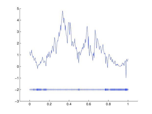
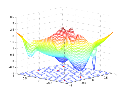
In Fig. 7, an example of convergence of the sequence of trial points generated by the algorithm MGAS in dimension using the approximation of the level to the Peano curve is given. The zone with the high density of the trial points corresponds to the global minimizer.
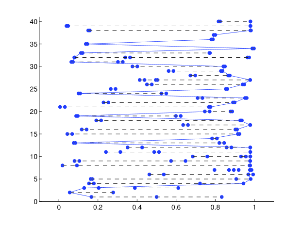
Fig. 8 shows how this problem was solved in the one-dimensional space. In the upper part of Fig. 8, the one-dimensional function corresponding to the curve shown in Fig. 7 and the respective trial points produced by the MGAS at the interval are presented. The lower part of the Figure shows the dynamics (from bottom to top) of 40 iterations executed by the MGAS. It can be seen that each iteration contains more than one trial. The piece-wise line connects points with the best function value obtained during that iteration.
In order to conclude this section it should be noticed that Theorem 3.3 establishes convergence conditions of infinite sequences of trial points generated by the algorithm MGAS to any point of the domain and therefore to the global minimum points of the one-dimensional function . The Peano curves used for reduction of dimensionality establish a correspondence between subintervals of the curve and the -dimensional subcubes of the domain . Every point on the curve approximates an -neighborhood in , i.e., the points in the -dimensional domain may be approximated differently by the points on the curve in dependence on the mutual disposition between the curve and the point in to be approximated (see [38, 40]). Here by approximation of a point we mean the set of points (called images) on the curve minimizing the Euclidean distance from . It was shown in [38, 40] that the number of the images ranges between and . These images can be located on the curve very far from each other despite their proximity in the -dimensional space. Thus, by using the space-filling Peano curve , the global minimizer in the -dimensional space can have up to images on the curve, i.e., it is approximated by , , points such that
where is defined by the space-filling curve. Obviously, in the limiting case, when and the iteration number , all global minimizers will be found. But in practice we work with a finite and , i.e., with a finite trial sequence, then to obtain an -approximation of the solution it is sufficient to find only one of the images on the curve. This effect may result in a serious acceleration of the search (see [40] for a detailed discussion).
4 Numerical experiments
In this section, we present results of numerical experiments performed to compare the new algorithm MGAS with the original DIRECT algorithm proposed in [15] and its locally biased modification LBDirect introduced in [7, 8]. These methods have been chosen for comparison because they, just as the MGAS method, do not require the knowledge of the objective function gradient and work with several Lipschitz constants simultaneously. The Fortran implementation of the two methods described in [7] and downloadable from [6] have been used in both methods.
To execute numerical experiments with the algorithm MGAS, we should define its parameter from (3.3). In DIRECT (see [15]), where a similar parameter is used, the value is related to the current minimal function value and is fixed as follows:
| (4.1) |
The choice of between and has demonstrated good results for DIRECT on a set of test functions (see [15]). Since the value has produced the most robust results for DIRECT (see, e.g., [7, 8, 15]), exactly this value was used in (4.1) for DIRECT in our experiments. The same formula (4.1) and the same value were used in the new algorithm, too.
The series of experiments involves a total of 800 test functions in
the dimensions generated by the GKLS-generator described
in [9] and downloadable from
http://wwwinfo.deis.unical.it/yaro/GKLS.html. More precisely,
eight classes of 100 functions have been considered.
The generator allows one to construct classes of randomly
generated
multidimensional and multiextremal test functions with
known values of local and global minima and their
locations. Each test class
contains 100 functions and only the following five parameters should be defined by the user:
– problem dimension;
– number of local minima;
– value of the global minima;
– radius of the attraction region of the
global minimizer;
– distance from the global minimizer to the
vertex of the paraboloid.
The generator works by constructing in a convex quadratic function, i.e., a paraboloid, systematically distorted by polynomials. In our numerical experiments we have considered classes of continuously differentiable test functions with local minima. The global minimum value has been fixed equal to for all classes. An example of a function generated by the GKLS can be seen in Fig. 9.
By changing the user-defined parameters, classes with different properties can be created. For example, a more difficult test class can be obtained either by decreasing the radius of the attraction region of the global minimizer or by increasing the distance, , from the global minimizer to the paraboloid vertex. In this paper, for each dimension , two test classes where considered: a simple one and a difficult one, see Table 1 that describes the classes used in the experiments. Since the GKLS-generator provides functions with known locations of global minima, the experiments have been carried out by using the following stopping criteria.
| Class | Difficulty | N | m | |||
|---|---|---|---|---|---|---|
| 1 | Simple | 2 | 10 | -1.0 | 0.90 | 0.20 |
| 2 | Hard | 2 | 10 | -1.0 | 0.90 | 0.10 |
| 3 | Simple | 3 | 10 | -1.0 | 0.66 | 0.20 |
| 4 | Hard | 3 | 10 | -1.0 | 0.90 | 0.20 |
| 5 | Simple | 4 | 10 | -1.0 | 0.66 | 0.20 |
| 6 | Hard | 4 | 10 | -1.0 | 0.90 | 0.20 |
| 7 | Simple | 5 | 10 | -1.0 | 0.90 | 0.40 |
| 8 | Hard | 5 | 10 | -1.0 | 0.90 | 0.30 |
Stopping criteria. If denotes the global minimizer of the -th function of the test class, , then the search terminates either when the maximal number of trials , equal to , was reached or when a trial point falls in a ball having a radius and the center at the global minimizer of the -th function of the class, i.e.,
| (4.2) |
All the methods under comparison can execute trials in the course of each -th iteration, therefore, when condition (4.2) is satisfied at an iteration the number of trials executed to solve the problem is calculated as . The radius from (4.2) in the stopping rule was fixed equal to for classes 1–6 and for classes 7 and 8.
| Class 1 | Class 5 | ||||
|---|---|---|---|---|---|
| Average | Maximal | Average | Maximal | ||
| 174.24 | 565 | 12174.20 | 171561 | ||
| 227.60 | 889 | 10674.30 | 95467 | ||
| 268.98 | 1279 | 15145.12 | 143075 | ||
In order to show the influence of the parameter introduced in (3.7) on the search, a sensitivity analysis has been performed. Two different classes of test functions have been considered: class 1 in and class 5 in (see Table 1). Three different values of the parameter were used for each class. In Table 2, the average and the maximal number of function evaluations calculated in order to satisfy the stopping rule for all 100 functions of each class are reported. Notice that the best results (shown in bold) were obtained for for the class 1, and for for the class 5. In the case of dimension , values of smaller than produce an intensification of the search in subintervals already well-explored. Conversely, when the dimension increases the reduced function in one dimension becomes more oscillating and it is necessary to reduce the value of the parameter . In general, if a too small value of the parameter is applied, the algorithm continues the search in parts of the domain that were already well-explored during the previous iterations. Obviously, if a too large value of is used it happens that from a certain iteration onward, no interval is selected for the subdivision and the global solution can be lost.
Taking into account results of the sensitivity analysis, the following values have been chosen: for classes 1 and 2, for the class 3, for the class 4 and for the classes 5–8.
In the algorithm MGAS, an -approximation of the Peano curve has been considered. In particular the level of the curve must be chosen taking in mind the constraint , where is the dimension of the problem and is the number of digits in the mantissa depending on the computer that is used for the implementation (see [34] for more details). In our experiments we had , thus the value has been used for all the classes of test functions.
Results of numerical experiments with the eight GKLS test classes from Table 1 are shown in Table 3. The columns “Average number of trials” in Table 3 report the average number of trials performed during minimization of the 100 functions from each GKLS class. The simbol “” reflects the situations when not all functions of a class were successfully minimized by the method under consideration: that is the method stopped when 1000000 trials had been executed during minimizations of several functions of this particular test class. In these cases, the value 1000000 was used in calculations of the average value, providing in such a way a lower estimate of the average. The columns “Maximal number of trials” report the maximal number of trials required for satisfying the stopping rule for all 100 functions of the class. The notation “1000000 ()” means that after 1000000 function evaluations the method under consideration was not able to solve problems.
| Class | Average number of trials | Maximal number of trials | ||||
|---|---|---|---|---|---|---|
| DIRECT | LBDirect | MGAS | DIRECT | LBDirect | MGAS | |
| 1 | 208.54 | 304.28 | 174.24 | 1159 | 2665 | 565 |
| 2 | 1081.42 | 1291.70 | 622.60 | 3201 | 4245 | 1749 |
| 3 | 1140.68 | 1893.02 | 1153.64 | 13369 | 20779 | 5267 |
| 4 | 42334.36 | 5245.72 | 2077.60 | 1000000(4) | 32603 | 9809 |
| 5 | 47768.28 | 21932.94 | 9961.70 | 1000000(4) | 179383 | 95467 |
| 6 | 95908.99 | 74193.53 | 21687.76 | 1000000(7) | 372633 | 319493 |
| 7 | 33878.09 | 31955.06 | 7306.04 | 1000000(3) | 146623 | 36819 |
| 8 | 149578.61 | 93876.77 | 23460.00 | 1000000(13) | 1000000(1) | 96287 |
Table 4 reports the ratio between the maximal (and average) number of trials performed by DIRECT and LBDirect with respect to the corresponding number of trials performed by the new algorithm MGAS. It can be seen from Table 4 that the algorithm MGAS outperforms both competitors significantly on the given test classes.
| Class | Average number of trials | Maximal number of trials | ||
|---|---|---|---|---|
| DIRECT/MGAS | LBDirect/MGAS | DIRECT/MGAS | LBDirect/MGAS | |
| 1 | 1.20 | 1.75 | 2.05 | 4.72 |
| 2 | 1.74 | 2.07 | 1.83 | 2.43 |
| 3 | 0.99 | 1.64 | 2.54 | 3.95 |
| 4 | 20.38 | 2.52 | 101.95 | 3.32 |
| 5 | 4.80 | 2.20 | 10.47 | 1.88 |
| 6 | 4.42 | 3.42 | 3.13 | 1.17 |
| 7 | 4.64 | 4.37 | 27.16 | 6.82 |
| 8 | 6.38 | 4.00 | 10.39 | 10.39 |
classes 1,3,5,7
classes 2,4,6,8
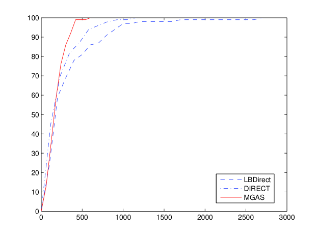
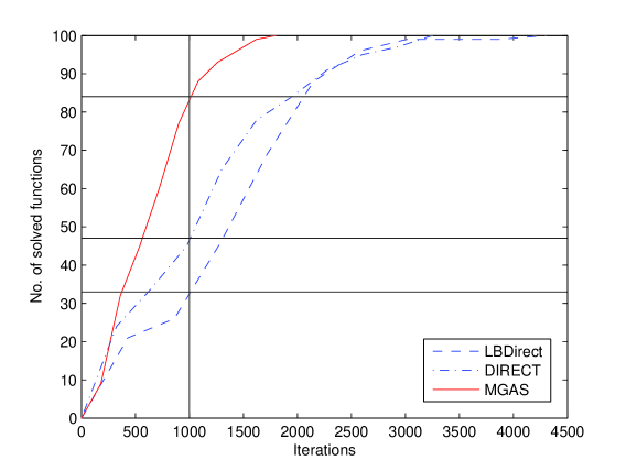
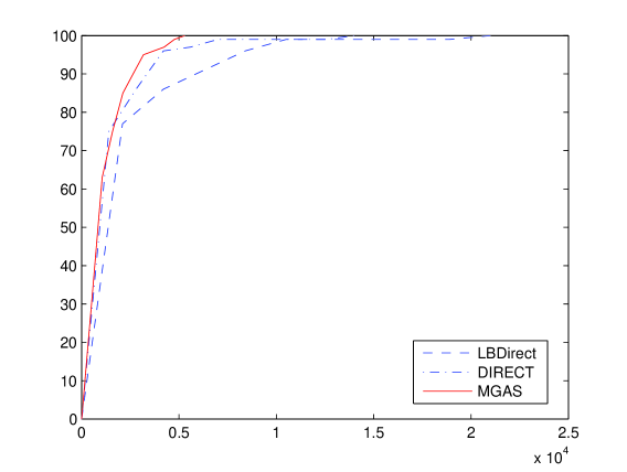
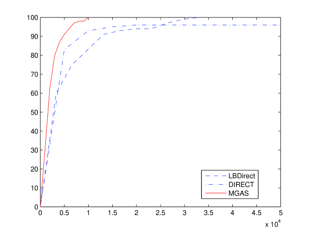
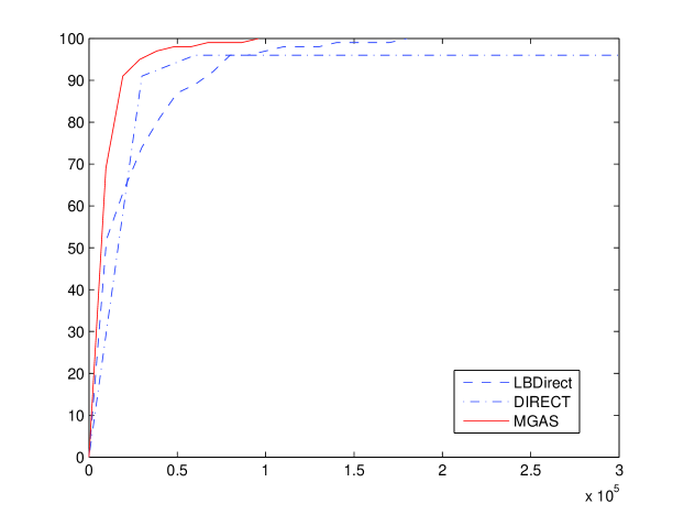
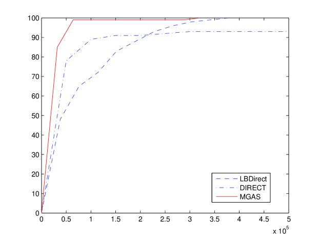
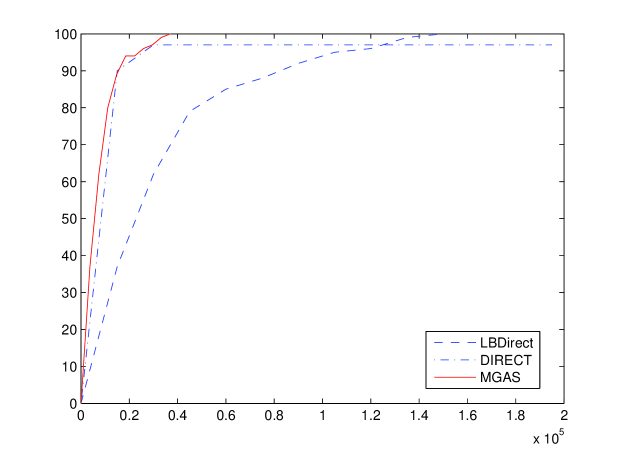
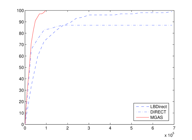
Figure 10 shows a comparison of the three methods using the so called operating characteristics introduced in 1978 in [14] (see, e.g., [40] for their English-language description). These characteristics show very well the performance of algorithms under the comparison for each class of test functions. On the horizontal axis we have the number of function evaluations and the vertical coordinate of each curve shows how many problems have been solved by one or another method after executing the number of function evaluations corresponding to the horizontal coordinate. For instance, the first graph in the right-hand column (, class 2) shows that after 1000 function evaluations the LBDirect has found the global solution at 33 problems, DIRECT at 47 problems, and the MGAS at 84 problems. Thus, the behavior of an algorithm is better if its characteristic is higher than characteristics of its competitors. In Figure 10, the left-hand column of characteristics, the behavior of algorithms MGAS, DIRECT, and LBDirect on the classes 1, 3, 5, and 7 is shown. The right-hand column presents the situation when the more difficult classes 2, 4, 6, and 8 have been used.
5 A brief conclusion
The global optimization problem of a multi-dimensional, non-differentiable, and multiextremal function has been considered in this paper. It was supposed that the objective function can be given as a ‘black-box’ and the only available information is that it satisfies the Lipschitz condition with an unknown Lipschitz constant over the search region being a hyperinterval in .
A new deterministic global optimization algorithm called MGAS has been proposed. It uses the following two ideas: the MGAS applies numerical approximations to space-filling curves to reduce the original Lipschitz multi-dimensional problem to a univariate one satisfying the Hölder condition; the MGAS at each iteration uses a new geometric technique working with a number of possible Hölder constants chosen from a set of values varying from zero to infinity evolving so ideas of the popular DIRECT method to the field of Hölder global optimization. Convergence conditions of the MGAS have been established. Numerical experiments carried out on 800 of test functions generated randomly have been executed.
It can be seen from the numerical experiments that the new algorithm shows quite a promising performance in comparison with its competitors. Moreover, the advantage of the new technique becomes more pronounced for harder problems.
References
- [1] Butz A.R., Space filling curves and mathematical programming, Information and Control, 12(4), 313–330 (1968).
- [2] Calvin J. and Žilinskas A., One-dimensional P-algorithm with convergence rate for smooth functions, J. of Optimization Theory and Applications, 106(2), 297–307 (2000).
- [3] Casado L.G., García I., and Sergeyev Ya.D., Interval algorithms for finding the minimal root in a set of multiextremal non-differentiable one-dimensional functions, SIAM J. on Scientific Computing, 24(2), 359–376 (2002).
- [4] Evtushenko Yu.G. and Posypkin M., A deterministic approach to global box-constrained optimization, Optimization Letters, 7(4), 819–829 (2013).
- [5] Famularo, D., Pugliese, P., and Sergeyev, Ya.D., A global optimization technique for checking parametric robustness, Automatica, 35, 1605-1611, (1999).
- [6] Gablonsky M.J., DIRECT v2.04 FORTRAN code with documentation, 2001, http://www4.ncsu.edu/ ctk/SOFTWARE/DIRECTv204.tar.gz.
- [7] Gablonsky M.J., Modifications of the DIRECT Algorithm, Ph.D thesis, North Carolina State University, Raleigh, NC, 2001.
- [8] Gablonsky M.J. and Kelley C.T., A locally-biased form of the DIRECT Algorithm, J. of Global Optimization, 21, 27–37 (2001).
- [9] Gaviano M., Kvasov D.E., Lera D., and Sergeyev Ya.D., Software for generation of classes of test functions with known local and global minima for global optimization, ACM TOMS, 29(4), 469–480 (2003).
- [10] Horst R. and Pardalos P.M., Handbook of Global Optimization, Kluwer, Doordrecht (1995).
- [11] Horst R. and Tuy H., Global Optimization: Deterministic Approaches, Springer, Berlin, (1996).
- [12] Gourdin E., Jaumard B., and Ellaia R., Global optimization of Hölder functions, J. of Global Optimization, 8, 323-348 (1996).
- [13] Gergel V.P., Sergeyev Ya.D. Sequential and parallel global optimization algorithms using derivatives, Computers Mathematics with Applications, 37(4-5), 163–180 (1999).
- [14] Grishagin V.A., Operating characteristics of some global search algorithms, Problems of Stochastic Search, Zinatne, Riga, 7, 198–206 (1978), (In Russian).
- [15] Jones D.R., Perttunen C.D., and Stuckman B.E., Lipschitzian optimization without the Lipschitz constant, J. of Optimization Theory and Applications, 79, 157–181 (1993).
- [16] Kvasov D.E., Pizzuti C., and Sergeyev Ya.D., Local tuning and partition strategies for diagonal GO methods, Numerische Mathematik, 94(1), 93–106 (2003).
- [17] Kvasov D.E. and Sergeyev Ya.D., A univariate global search working with a set of Lipschitz constants for the first derivative, Optim. Letters, 3, 303–318 (2009).
- [18] Kvasov D.E. and Sergeyev Ya.D., Lipschitz gradients for global optimization in a one-point-based partitioning scheme, J. of Computational and Applied Mathematics, 236(16), 4042–4054 (2012).
- [19] Kvasov D.E. and Sergeyev Ya.D., Lipschitz global optimization methods in control problems, Automation and Remote Control, 74(9), 1435–1448 (2013).
- [20] Kvasov D.E. and Sergeyev Ya.D., A deterministic global optimization using smooth diagonal auxiliary functions, Communications in Nonlinear Science and Numerical Simulation, (to appear).
- [21] Lera D. and Sergeyev Ya.D., Global minimization algorithms for Hölder functions, BIT, 42(1), 119–133 (2002).
- [22] Lera D. and Sergeyev Ya.D., An information global minimization algorithm using the local improvement technique, J. of Global Optimization, 48, 99–112 (2010).
- [23] Lera D. and Sergeyev Ya.D., Lipschitz and Hölder global optimization using space-filling curves, Appl. Numer. Maths., 60, 115–129 (2010).
- [24] Lera D. and Sergeyev Ya.D., Acceleration of univariate global optimization algorithms working with Lipschitz functions and Lipschitz first derivatives, SIAM J. Optim., 23(1), 508–529 (2013).
- [25] Martínez J.A., Casado L.G., García I., Sergeyev Ya.D., Toth B. On an efficient use of gradient information for accelerating interval global optimization algorithms, Numerical Algorithms, 37, 61–69 (2004).
- [26] Paulavičius R., Sergeyev Ya.D., Kvasov D.E. and Žilinskas J. Globally-biased Disimpl algorithm for expensive global optimization, J. of Global Optimization, 59(2-3), 545–567 (2014).
- [27] Paulavičius R. and Žilinskas J., Simplicial Global Optimization, Springer, New York (2014).
- [28] Pintér J.D., Global Optimization in Action, Kluwer, Dordrecht (1996).
- [29] Piyavskii S.A., An algorithm for finding the absolute extremum of a function, USSR Comput. Math. and Math. Phys., 12, 57–67 (1972).
- [30] Preparata F.P. and Shamos M.I., Computational Geometry: An Introduction, Springer–Verlag, New York (1993).
- [31] Sagan H., Space-Filling Curves, Springer, New York (1994).
- [32] Sergeyev Ya.D., An information global optimization algorithm with local tuning, SIAM J. Optim., 5, 858–870 (1995).
- [33] Sergeyev Ya.D., On convergence of “Divide the Best” global optimization algorithms, Optimization, 44(3), 303–325 (1998).
- [34] Sergeyev Ya.D., Global one-dimensional optimization using smooth auxiliary functions, Mathematical Programming, 81(1), 127–146 (1998).
- [35] Sergeyev Ya.D., Daponte P., Grimaldi D., and Molinaro A., Two methods for solving optimization problems arising in electronic measurements and electrical engineering, SIAM J. Optim., 10(1), 1–21 (1999).
- [36] Sergeyev Ya.D. and Kvasov D.E. Global search based on efficient diagonal partitions and a set of Lipschitz constants, SIAM J. Optim. 16(3), 910–937 (2006).
- [37] Sergeyev Ya.D. and Kvasov D.E., Diagonal global optimization methods, Fizmatlit, Moscow (2008), (in Russian).
- [38] Sergeyev Ya.D., Strongin R.G., and Lera D., Introduction to Global Optimization Exploiting Space-Filling Curves, Springer, New York (2013).
- [39] Strongin R.G., Numerical Methods in Multiextremal Problems: Information-Statistical Algorithms, Nauka, Moscow (1978), (In Russian).
- [40] Strongin R.G. and Sergeyev Ya.D., Global Optimization with Non-convex Constraints: Sequential and Parallel Algorithms, Kluwer, Dordrecht (2000).
- [41] Strongin R.G. and Sergeyev Ya.D., Global optimization: fractal approach and non-redundant parallelism, J. of Global Optimization, 27(1), 25–50 (2003).
- [42] Zhigljavsky A.A. and Žilinskas A., Stochastic Global Optimization, Springer, New York, 2008.
- [43] Žilinskas, A. On similarities between two models of global optimization: statistical models and radial basis functions, J. of Global Optimization, 48(1), 173–182 (2010).
- [44] Žilinskas, A. and Žilinskas J. Interval Arithmetic Based Optimization in Nonlinear Regression, Informatica, 21(1), 149–158 (2010).