Computational Analysis of Amoeboid Swimming at Low Reynolds Number

Abstract

Recent experimental work has shown that eukaryotic cells can swim in a fluid as well as crawl on a substrate. We investigate the swimming behavior of Dictyostelium discoideum  amoebae who swim by initiating traveling protrusions at the front that propagate rearward. In our model we prescribe the velocity at the surface of the swimming cell, and use techniques of complex analysis to develop $2$D models that enable us to study the fluid-cell interaction. Shapes that approximate the protrusions used by Dictyostelium discoideum  can be generated via the Schwarz-Christoffel transformation, and the boundary-value problem that results for swimmers in the Stokes flow regime is then reduced to an integral equation on the boundary of the unit disk. We analyze the swimming characteristics of several varieties of swimming Dictyostelium discoideum  amoebae, and discuss how the slenderness of the cell body and the shapes of the protrusion effect the swimming of these cells. The results may provide guidance in designing low Reynolds number swimming models.

1 Introduction

Cell locomotion is essential throughout the development and adult forms of uni- and multi-cellular organisms. It is beneficial in various types of taxis, in morphogenetic movements during development, and in the immune response and wound healing in adults, but it plays a deleterious role in cancer metastasis. When movement is in response to extracellular signals, it involves the detection and transduction of those signals, which can be biochemical, mechanical or of other types, the integration of the signals into an intracellular signal, and the spatio-temporal control of the intracellular biochemical and mechanical responses that lead to force generation, morphological changes and directed movement (Sheetz et al., 1999). Many single-celled organisms use flagella or cilia to swim, and many mathematical models of swimming in such organisms have been developed (Lauga & Powers, 2009). The movements of eukaryotic cells that lack such structures fall into two broad categories: mesenchymal and amoeboid (Binamé et al., 2010). The former can be characterized as ‘crawling’ in fibroblasts or ‘gliding’ in keratocytes, and involves the extension of either pseudopodia and/or lamellipodia driven by actin polymerization at the leading edge. This mode dominates in cells such as fibroblasts when moving on a 2D substrate. On flat surfaces the predominant protrusions are lamellipodia and these processes suffice, but in the extracellular matrix (ECM) the protrusions and cell body are more rounded, and the cells may also secrete matrix-degrading proteases (MMPs) and ‘tunnel’ their way through the ECM (Martins & Kolega, 2006, Mantzaris et al., 2004).

In the amoeboid mode cells are more rounded, and move through the ECM by avoiding obstacles when possible, rather than removing them. Thus they rely less on attachment to the ECM and degradation of it, and instead exploit variations in the ECM to move through it by shape changes. In this mode force transmission to the extracellular matrix (ECM) depends on shape changes driven by localized remodeling of the cytoskeleton (CSK) and myosin contraction (Insall & Machesky, 2009). Cells such as leukocytes, which normally use the mesenchymal mode in the ECM, can migrate in vivo in the absence of integrins, using a ’flowing and squeezing’ mechanism (Lämmermann et al., 2008). The human parasite Entamoeba histolytica uses an extreme form of amoeboid movement called blebbing, in which the membrane detaches from the CSK (Maugis et al., 2010), whereas zebrafish primordial germ cells and Dictyostelium discoideum  (Dd) cells move using a combination of blebbing and protrusion by spatio-temporal control of the membrane attachment to the CSK (Blaser et al., 2006, Diz-Muñoz et al., 2010, Yoshida & Soldati, 2006, Zatulovskiy et al., 2014). Cells using this mode can move up to forty times faster than those using strong adhesion (Renkawitz & Sixt, 2010). Recent experiments have shown that numerous cell types display enormous plasticity in locomotion in that they sense the mechanical properties of their environment and adjust the balance between the modes by altering the balance between parallel signal transduction pathways (Renkawitz et al., 2009, Renkawitz & Sixt, 2010). Thus crawling and swimming are the extremes on a continuum of locomotion strategies, but many cells sense their environment and use the most efficient strategy in a given context.

Heretofore mathematical modeling has focused primarily on either the mesenchymal mode, in which cells crawl via attachments to a substrate (Danuser et al., 2013), or on microorganisms that swim using flagella or cilia (Suarez & Pacey, 2006, Berg & Anderson, 1973, Lowe et al., 1987, Gibbons, 1981, Sleigh et al., 1988, Ishimoto & Gaffney, 2014). Here we analyze swimming of larger cells, motivated by recent experiments which show that both neutrophils and Dd can swim – in the strict sense of propelling themselves through a fluid using only fluid-cell interactions – in response to chemotactic gradients (Barry & Bretscher, 2010, Bae & Bodenschatz, 2010, Van Haastert, 2011). A basic question that arises is what pattern of shape changes are effective in propelling a cell. It has been reported (Salbreux et al., 2007) that freely suspended Swiss-3T3 fibroblast cells without cell-substrate adhesion can exhibit oscillatory shape dynamics, and some of them may also exhibit periodic bleb dynamics correlating with the oscillations, where blebs are hemispherical membrane blisters induced by cortical contraction (Fackler & Grosse, 2008, Paluch et al., 2005). The combination of both dynamics may result in a random oscillation of the cell in space. In comparison with such random motion, Dictyostelium and neutrophils can utilize the amoeboid swimming mode in which the cell body is elongated and small protrusions that provide the momentum transfer needed for motion are propagated from front to rear (Barry & Bretscher, 2010, Bae & Bodenschatz, 2010, Van Haastert, 2011).

In the following section we formulate the basic problem of swimming by shape deformations in 2D at low Reynolds number, which is the relevant regime for single cell movement. In 2D one can introduce a stream function, which leads to a biharmonic equation, and the general solution of the Stokes problem is expressed in terms of two analytic functions – the Goursat functions – that are determined by the motion of the boundary of the swimmer (Bouffanais et al., 2013, Chambrion & Munnier, 2011, Cherman et al., 2000). This in turn leads to an integral equation for one of these functions, and the second function can then be expressed in terms of the first. In Section 4 we study the motion of Dd in 2D, and approximate the shape changes using polygonal approximations. Using the Schwarz-Christoffel transformation, we reduce the problem to the solution of a linear system of equations for basis functions on the boundary of the unit disk. We show that realistic propagating shapes can produce propulsion at speeds in the range observed experimentally using realistic choices of the parameters.

Since cell movement, whether on a solid substrate, in a fluid, or in a complex medium such as the ECM, involves the interplay between biochemical and mechanical processes, dissecting the roles of each is a first step toward an integrated description of movement. A major objective of our work is to answer a question posed by experimentalists, which is ‘How does deformation of the cell body translate into locomotion?’ (Renkawitz & Sixt, 2010). A longer-range goal is to produce a unified description for swimming that integrates signaling and mechanics in viscous and viscoelastic environments similar to the extracellular tissue environment. As one experimentalist stated ’the complexity of cell motility and its regulation, combined with our increasing molecular insight into mechanisms, cries out for a more inclusive and holistic approach, using systems biology or computational modeling, to connect the pathways to overall cell behavior’ (Insall & Machesky, 2009).

2 Low Reynolds Number Swimming Problems

2.1 General description of swimming mechanics at low Reynolds numbers

Recent interest in the motion of biological organisms in a viscous fluid was re-kindled by Purcell’s 1977 description of life at low Reynolds number (LRN) (Purcell, 1977), and a wide variety of applications have been analyzed since then. A review of some of these is given elsewhere (Lauga & Powers, 2009), and we only describe the relevant background. We consider motion in an incompressible Newtonian fluid of density $\rho$, viscosity $\mu$, and velocity ${\bm{u}}$, for which the governing equations are

$$\rho\dfrac{\partial{\bm{u}}}{\partial t}+\rho({\bm{u}}\cdot\nabla){\bm{u}} =\nabla\cdot\mbox{$\mathbb{T}$}+{\mbox{\bm{$f$}}}=-\nabla p+\mu\Delta{\bm{u}}+{\mbox{\bm{$f$}}},$$ (2.1)

$$\nabla\cdot{\bm{u}} =0$$ (2.2)

where $\mbox{$\mathbb{T}$}=-p{\mbox{\bm{$\delta$}}}+\mu(\nabla{\bm{u}}+(\nabla{\bm{u}})^{T})$ is the viscous stress tensor. ${\bf f}$ is the external force field, which we assume to be zero or include it in the pressure hereafter. This is appropriate for the experimental configuration described in (Barry & Bretscher, 2010), since the fluid had a variable density that allowed cells to find a point of neutral buoyancy. The Reynolds number based on a characteristic length scale $L$ and speed scale $U$ is Re = $\rho LU/\mu$, and when converted to dimensionless form and the symbols re-defined, the equations read

$$Re\cdot\!Sl\dfrac{\partial{\bm{u}}}{\partial t}+Re({\bm{u}}\cdot\nabla){\bm{u}} = -\nabla p+\Delta{\bm{u}}$$ (2.3)

$$\nabla\cdot{\bm{u}} = 0.$$

Here $Sl=\omega L/U$ is the Strouhal number and $\omega$ is a characteristic frequency of the shape changes. When Re$\,\ll 1$ the convective momentum term in (2.3) can be neglected, but the time variation requires that $Re\cdot\!Sl\equiv\omega L^{2}/\nu\ll 1$. This is not always true, even for small swimmers (Ishimoto, 2013, Wang & Ardekani, 2012), but as we show next, it applies here.

The small size and slow speed of cells considered here leads to LRN flows, and in this regime cells move by exploiting the viscous resistance of the fluid. For example, Dd amoebae have a typical length $L\sim 25\mu\textrm{m}$ and can swim at $U\sim 3\mu\textrm{m}/\textrm{min}$ (Van Haastert, 2011). Assuming the medium is water $(\rho\sim 10^{3}\textrm{kg}\ \textrm{m}^{-3},\ \mu\sim 10^{-3}\,\textrm{Pa-s})$, and the deformation frequency $\omega\sim 1/s$, $Re\sim{\mathcal{O}}(10^{-6})$ and $Sl\sim{\mathcal{O}}(10^{-4})$. In fact the experiments are done in oil that is significantly more viscous (Barry & Bretscher, 2010). In any case, when both inertial terms on the left hand side of (2.3) are neglected, which we assume hereafter, the flow is governed by the Stokes equations

$$\mu\Delta{\bm{u}}-\nabla p={\bf 0},\qquad\qquad\nabla\cdot{\bm{u}}=0.$$ (2.4)

Throughout we consider the propulsion problem in an infinite domain and assume that the fluid is at rest at infinity.

Since time does not appear in the equations, a time-reversible stroke produces no net motion, which is the content of the famous ‘scallop theorem’ (Purcell, 1977). Furthermore, since we assume that there is no inertia in the fluid (momentum transfer is assumed to be instantaneous), in the Stokes regime there is no net force or torque on a self-propelled swimmer moving in an infinite fluid that is at rest at infinity. One can see this by integrating the stress over the boundary of the swimmer and then equating this via the momentum equation to the stress on a circle at infinity (Shapere & Wilczek, 1989b ). Therefore movement is a purely geometric process: the net displacement of a swimmer during a stroke is independent of the rate at which the stroke is executed when $Re=0$, and approximately so as long as $Re\cdot\!Sl$ remains small enough.

Let $\Omega(t)\in R^{n}$ be the swimmer (a compact set with a sufficiently smooth boundary). Throughout we consider a fixed global reference frame $(\bm{x},t)$ and a body frame $(\bm{X},t)$ attached to the swimmer, where time is scaled the same in both frames. We use the notation $\partial\Omega_{\bm{x}}(t)$ and $\partial\Omega_{\bm{X}}(t)$ to denote the boundary of $\Omega$ in the fixed and body frames, resp., and when observed from the body frame, the shape deformations of the swimmer are specified as $\bm{u}_{\textrm{s}}(\bm{X},t)$ for $\bm{X}\in\partial\Omega_{\bm{X}}(t)$. Denote the uniform (rigid-body) translational and rotational velocities of the swimmer when observed from the fixed frame as $\bm{U}(t)$ and $\bm{\omega}(t)$, respectively. Then the instantaneous velocity on the swimmer’s surface $\partial\Omega_{\bm{x}}(t)$ is

$$\bm{u}(\bm{x},t)=\bm{U}(t)+\bm{\omega}(t)\times\bm{x}+\bm{u}_{\textrm{s}}(\bm{X},t)$$ (2.5)

where $\bm{u}$ satisfies (2.4).

A swimming stroke is specified by a time-dependent sequence of shapes, and it is cyclic if the initial and final shapes are identical (Shapere & Wilczek, 1989b ). The canonical LRN self-propulsion problem is – given a cyclic shape deformation specified by $\bm{u}_{s}$, solve the Stokes equations subject to the zero force and torque conditions

$$\bm{F}(t)\equiv\int_{\partial\Omega_{\bm{x}}(t)}\mathbb{T}\cdot\mathbf{\mathsf{n}}=0,\qquad\bm{T}(t)\equiv\int_{\partial\Omega_{\bm{x}}(t)}{\bm{x}}\wedge(\mathbb{T}\cdot\mathbf{\mathsf{n}})=0$$ (2.6)

and the boundary conditions

$$\bm{u}|_{\partial\Omega}=\bm{u}_{\textrm{s}}+{\mbox{\bm{$U$}}}+\bm{\omega}\times\bm{x},\qquad\bm{u}|_{\bm{x}\rightarrow\infty}=\bm{0}$$ (2.7)

where $\mathbf{\mathsf{n}}$ is the exterior normal.

How does the swimmer move if force- and torque-free? It would appear that at best it can only translate or rotate at a constant rate. However, an arbitrary deformation of the surface will not satisfy (2.6) in general, and in particular, will generate a flow at infinity. However, since we assume that the fluid is at rest there this flow must be counteracted by an imposed flow, which then defines the rigid linear and angular velocities of the swimmer, and leads to satisfaction of the force-free and torque-free conditions (Shapere & Wilczek, 1989b ). Since the shape changes are time-dependent the counterflow is also, as are the rigid translations and rotations.

Thus the canonical LRN swimming problem is: given a cyclic sequence of shape deformations by specifying $\bm{u}_{\textrm{s}}$ on the boundary $\partial\Omega_{\bm{X}}$ of the swimmer, solve the Stokes equations (2.4) for a trial velocity field $\bm{u}$ and then use the force-free and torque-free conditions to determine $\bm{U}$ and $\bm{\omega}$ so as to satisfy the boundary conditions at infinity. In what follows we restrict attention to swimming in two space dimensions, and describe the problem as the 2D LRN swimming (2DLRNS) problem.

2.2 The 2D swimmer

In two space dimensions techniques from complex analysis can be used to significantly simplify the problem of computing solutions to the Stokes equations for LRN swimming problems. Two main methods have been developed that can be applied, one that was first developed by Muskhelishvili to solve problems in elasticity (Muskhelishvili, 1977), and another that is essentially a boundary integral method(Pozrikidis, 1992) for 2D problems (Greengard et al., 1996, Kropinski, 1999; 2001; 2002, Kropinski & Lushi, 2011). Significant analytical insights can be gained using Muskhelishvili’s method, including the application of control theory to LRN swimming (Shapere & Wilczek, 1989b , Shapere & Wilczek, 1989a , Kelly, 1998, Kelly & Murray, 2000), and we use this method in this paper.

In $2D$ the incompressibility condition $\nabla\cdot\bm{u}=0$ in (2.4) can be satisfied by introducing a stream function $\Lambda(z,\overline{z};t)$, which is a real-valued scalar potential such that

$$u=\dfrac{\partial\Lambda}{\partial y}-i\dfrac{\partial\Lambda}{\partial x}.$$

Here and hereafter we use $u\in\mathbb{C}$ to denote the velocity field (denoted by $\bm{u}$ in Section 2.1) in the complex $z$-plane. Then the Stokes equations (2.4) imply that $\Lambda$ satisfies the biharmonic equation

$$\Delta^{2}\Lambda=0.$$ (2.8)

The general solution of (2.8) can be expressed by Goursat’s formula (Muskhelishvili, 1977)

$$\Lambda(z,\overline{z};t)=\Re\big{[}\bar{z}\phi(z;t)+\chi(z;t)\big{]}$$ (2.9)

where for any $t$, $\phi(z;t)$ and $\chi(z;t)$ are analytic functions on the fluid domain $\mathbb{C}\setminus\Omega(t)$ and continuous on $\mathbb{C}\setminus\textrm{int}\Omega(t)$, where $\textrm{int}\,\Omega$ denotes the interior of $\Omega$. $\phi(z;t)$ and $\chi(z;t)$ are the Goursat functions. To simplify the expression of physical quantities and the following discussion, we hereafter impose the substitution $\phi\rightarrow-i\phi$, $\chi\rightarrow-i\chi$, as suggested by Shapere and Wilczek (Shapere & Wilczek, 1989b ), and Table 1 gives the expressions of several physical quantities in terms of these functions. In the table and hereafter we denote $\partial_{z}$ by ^′ for simplicity, $n=-idz/ds$ gives the exterior normal to $\partial\Omega$ (i.e., directed into the fluid domain), and $s$ denotes the arc length, traversed counterclockwise.

Table 1: Representation of various physical quantities by the Goursat functions.

Velocity	$u=\phi(z)-z\overline{\phi^{\prime}(z)}-\overline{\chi^{\prime}(z)}$
Pressure	$p=-4\mu\Re\{\phi^{\prime}(z)\}$
Vorticity	$\vartheta=-4\Im\{\phi^{\prime}(z)\}$
Stress force	$f=4\mu\Re(\phi^{\prime})n-2\mu(z\overline{\phi^{\prime\prime}}+\overline{\chi^{\prime\prime}})\overline{n}$
Stress force	$fds=-2i\mu d\big{(}\phi+z\overline{\phi^{\prime}}+\overline{\chi^{\prime}}\big{)}$
(differential form)

For swimming problems in a $2D$ Stokes flow in the unbounded domain $\mathbb{C}/\Omega(t)$, we require that the stress vanish at infinity, and as a result the Goursat functions must take the general form (Muskhelishvili, 1977, Greengard et al., 1996):

$$\phi(z,t) = -\dfrac{X(t)+iY(t)}{2\pi(1+\kappa(t))}\log z+\widetilde{\phi}(z,t)$$ (2.10)

$$\psi(z,t)=\chi^{\prime}(z,t) = \dfrac{X(t)-iY(t)}{2\pi(1+\kappa(t))}\log z+\widetilde{\psi}(z;t)$$ (2.11)

where $\widetilde{\phi}(z,t)$ and $\widetilde{\psi}(z,t)$ are single-valued and analytic on $\overline{\mathbb{C}}/\Omega$ (where $\overline{\mathbb{C}}=\mathbb{C}\cup\{\infty\}$). For the self-propulsion problem we must also require that $X=Y=0$ to ensure a bounded velocity at infinity. We then compute the translational and rotational velocity for a trial pair $(\widetilde{\phi},\widetilde{\chi})$, and when these are subtracted from the flow the motion is force-free and torque-free (Muskhelishvili, 1977, Greengard et al., 1996). Thus for $2$D swimming problems, the Goursat functions $\phi(z)$ and $\psi(z)$ should be single-valued and analytic on $\overline{\mathbb{C}}/\Omega$, and therefore they have Laurent expansions in $\overline{\mathbb{C}}/\Omega$ of the following form.

$$\phi(z,t) = a_{0}(t)+\dfrac{a_{-1}(t)}{z}+\dfrac{a_{-2}(t)}{z^{2}}+\cdots$$ (2.12)

$$\psi(z,t) = b_{0}(t)+\dfrac{b_{-1}(t)}{z}+\dfrac{b_{-2}(t)}{z^{2}}+\cdots$$ (2.13)

As a result, the 2DLRNS problem with specified shape changes as described above can be rephrased as follows – find functions $\phi(z,t)$ and $\psi(z,t)$ that are analytic on $\overline{\mathbb{C}}/\Omega(t)$ and continuous on $\overline{\mathbb{C}}/\textrm{int}\;\Omega(t)$ such that

$$\phi(z,t)-z\overline{\phi^{\prime}(z;t)}-\overline{\psi(z,t)}=V(z,\overline{z},t)\qquad(z\in\partial\Omega(t)).$$ (2.14)

Here $V(z,\overline{z},t)$ for $z\in\partial\Omega(t)$ is the velocity boundary condition determined by the shape changes, namely, the complex form of $\bm{u}_{\textrm{s}}$ as introduced in Section 2.1. Equation (2.14) will be referred to as the boundary condition constraint on $\phi$ and $\psi$ in the study of 2D LRN swimming.

2.3 Pull-back of the problem to the disk and derivation of the Fredholm integral equation

As we mentioned earlier, there are two main methods for solving the 2D LRN problem – which is to say to solve (2.14) – Muskhelishvili’s method and the integral equation method. In the integral equation method the velocity boundary condition leads to an integral operator defined on the swimmer’s boundary, while in Muskhelishvili’s method the approach is to first map the $z$-plane to a fixed complex computational $\zeta$-plane, on which the integral operator is applied. In the first case one deals with a moving boundary whose stress field is specified, while in Muskhelishvili’s method we consider velocity boundary condition and the problem can be pulled back into a fixed boundary problem. Generally speaking, the integral equation method is useful when the stress field along the boundary is known or multiple bodies are involved. On the other hand, for a single deformable swimmer it is easier to treat a sequence of shape deformations using Muskhelishvili’s method, which also facilitates the use of control theory to 2D LRN swimming systems and simplifies the design and study of micro aquatic robots. Hereafter we focus on the use of Muskhelishvili’s method.

Suppose that the cell occupies an open, simply-connected, bounded region $\Omega(t)$ in the complex $z$-plane at time $t$. Let $D=\{\zeta\in\mathbb{C}:|\zeta|<1\}$ be the unit disk in the computational $\zeta$-plane. The regions exterior to $\overline{D}$ and to $\overline{\Omega}(t)$ in the extended complex planes, i.e., $\overline{\mathbb{C}}/\overline{D}$ and $\overline{\mathbb{C}}/\overline{\Omega}(t)$, are both simply-connected as the infinity point $\infty$ is included in $\overline{\mathbb{C}}$. The Riemann mapping theorem (Ahlfors, 1978) ensures the existence of a single-valued analytic conformal mapping $z=w(\zeta;t)$ which maps $\overline{\mathbb{C}}/\overline{D}$ one-to-one and onto $\overline{\mathbb{C}}/\overline{\Omega}(t)$, and preserves the correspondence of infinity, i.e., $w(\infty;t)\equiv\infty$. Moreover, this mapping can be extended continuously to $\overline{\mathbb{C}}/D$ (Younes, 2010), and $w$ maps $\partial(\overline{\mathbb{C}}/D)=S^{1}$ to $\partial\Omega(t)$.

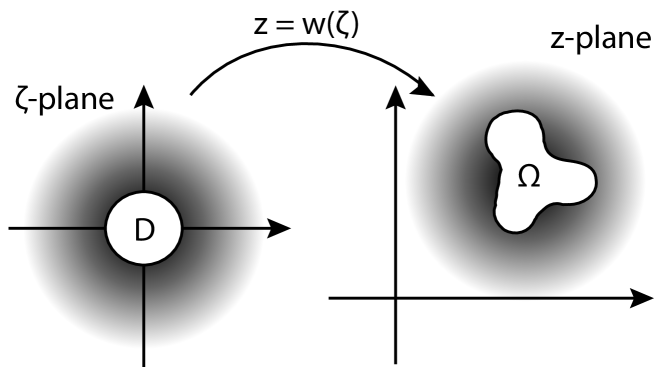
Figure 2.1: The conformal mapping from $\overline{\mathbb{C}}/D$ to $\overline{\mathbb{C}}/\Omega$.

We assume that the mapping preserves the point at infinity, and then have the following result regarding the form of its Laurent expansion (Ahlfors, 1978).

Lemma 1

Suppose that $\Omega(t)$ is a non-empty open bounded simply-connected domain in $\mathbb{C}$, and that $z=w(\zeta;t)$ is a conformal mapping from the exterior of the unit disk $D$ to $\Omega^{c}$ that preserves the point at infinity. Then $w(\zeta;t)$ has a Laurent expansion of the form

$$w(\zeta;t)=\alpha_{1}(t)\zeta+\alpha_{0}(t)+\dfrac{\alpha_{-1}(t)}{\zeta}+\dfrac{\alpha_{-2}(t)}{\zeta^{2}}+\cdots\dfrac{\alpha_{-n}(t)}{\zeta^{n}}+\cdots$$ (2.15)

where $\alpha_{1}(t)\neq 0\ \textrm{and}\ |\zeta|>1$.

When we consider in the body frame, $\Omega(t)$ gives the configuration of the swimmer, in which case we require $\alpha_{0}=0$ and $\alpha_{-1}\in\mathbb{R}$ in (2.15).

Hereafter $w(\zeta;t)$ is the conformal map which maps $\overline{\mathbb{C}}/\overline{D}$ onto $\overline{\mathbb{C}}/\Omega(t)$ such that $w(\infty;t)\equiv\infty$, extended to the boundary of the swimmer, which is given by $\partial\Omega(t)=\{z(t)=w(\sigma;t);\sigma\in S^{1}\}$. We impose a no-slip condition on the boundary, and therefore

$$u\big{(}w(\sigma)\big{)}(t)=\dfrac{\partial}{\partial t}w(\sigma;t).$$ (2.16)

Suppose that $\phi(z,t)$ and $\psi(z,t)$ are the solutions to the boundary condition constraint given by (2.14). Let

$$\Phi(\zeta;t)=\phi(w(\zeta;t);t),\qquad\Psi(\zeta)=\psi(w(\zeta;t);t)\qquad(|\zeta|\geq 1)$$

thus $\Phi(\zeta;t)$ and $\Psi(\zeta;t)$ are functions on $\zeta$-plane which are analytic on $\mathbb{C}/\overline{D}$ and continuous on $\mathbb{C}/D$ at any time $t$. Hence on $|\zeta|\geqslant 1$, we have Laurent expansion for $\Phi$ and $\Psi$ given by

$$\Phi(\zeta;t) = A_{0}(t)+\dfrac{A_{-1}(t)}{\zeta}+\dfrac{A_{-2}(t)}{\zeta^{2}}+\cdots$$ (2.17)

$$\Psi(\zeta;t) = B_{0}(t)+\dfrac{B_{-1}(t)}{\zeta}+\dfrac{B_{-2}(t)}{\zeta^{2}}+\cdots$$ (2.18)

where $A_{k},B_{k}$ ($k=0,-1,-2,\cdots$) are continuous functions from $[0,\infty]$ to $\mathbb{C}$.

If we substitute these expressions into (2.14) and omit the time index $t$, then the velocity field can be expressed as a function on the $\zeta$-plane as

$$\widetilde{u}(\zeta,\overline{\zeta}):=u\big{(}w(\zeta),\overline{w(\zeta)}\big{)}=\Phi(\zeta)-\dfrac{w(\zeta)}{\overline{w^{\prime}(\zeta)}}\overline{\Phi^{\prime}(\zeta)}-\overline{\Psi(\zeta)}$$ (2.19)

where ^′ represents $\partial_{\zeta}$. If we let $V(\sigma;t)$ denote the boundary condition of the velocity in general, then the boundary condition constraint (2.14) can be generalized to the condition

$$\Phi(\sigma)-\dfrac{w(\sigma)}{\overline{w^{\prime}(\sigma)}}\overline{\Phi^{\prime}(\sigma)}-\overline{\Psi(\sigma)}=V(\sigma)\qquad(\sigma\in S^{1}).$$ (2.20)

In the 2DLRNS problem the boundary condition is given as in (2.16), i.e., $V(\sigma;t)=\partial_{t}w(\sigma;t)$, but in the discussion below we will adopt the more general form $V(\sigma;t)=\sum_{n}\lambda_{n}(t)\sigma^{n}$.

Equation (2.20) involves both $\Phi$ and $\Psi$, but this can be reduced to an integral equation in $\Phi$ alone using a technique developed in Muskhelishvili, (1977), where it was originally developed for the solution of problems in elasticity rather than the Stokes flows, and the resulting integral equation is the same. We present the precise statement here for completeness. The reduction relies on a decomposition of the boundary condition $V(\sigma)$ derived from the following Plemelj formula (Sokhotskii, 1873, Cima & Ross, 2006, England, 2012).

Theorem 1 (Plemelj Formula)

Suppose $V(\sigma)$ is continuous on $S^{1}=\{\sigma\in\mathbb{C};|\sigma|=1\}$ and, for a particular $\sigma_{0}\in S^{1}$, satisfies the Hölder condition

$$\big{|}V(\sigma)-V(\sigma_{0})\big{|}\leq C\big{|}\sigma-\sigma_{0}\big{|}^{\alpha},\qquad\sigma\in S^{1}$$ (2.21)

for some positive constants $C$ and $\alpha$. Let

$$\widehat{V}(\zeta)=\dfrac{1}{2\pi i}\int_{S^{1}}\dfrac{V(\sigma)}{\sigma-\zeta}d\sigma$$ (2.22)

for $\zeta\in\mathbb{C}/S^{1}$. Then the limits

$$V^{-}(\sigma_{0}):=\lim_{r\rightarrow 1^{-}}\widehat{V}\big{(}r\sigma_{0}\big{)}\qquad\textrm{and}\qquad V^{+}(\sigma_{0}):=\lim_{r\rightarrow 1^{-}}\widehat{V}(\sigma_{0}/r)$$ (2.23)

exist and moreover, $V^{-}(\sigma_{0})-V^{+}(\sigma_{0})=V(\sigma_{0})$. Furthermore, the Cauchy principal-value integral

$$P.V.\int_{S^{1}}\dfrac{V(\sigma)}{\sigma-\sigma_{0}}d\sigma:=\lim_{\varepsilon\rightarrow 0}\int_{|\sigma-\sigma_{0}|>\varepsilon}\dfrac{V(\sigma)}{\sigma-\sigma_{0}}d\sigma$$

exists and

$$V^{+}(\sigma_{0})+V^{-}(\sigma_{0})=\dfrac{1}{\pi i}P.V.\int_{S^{1}}\dfrac{V(\sigma)}{\sigma-\sigma_{0}}d\sigma$$

We assume that the boundary condition $V(\sigma)$ in the swimming problems satisfies the Hölder condition as in (2.21) for any $\sigma_{0}\in S^{1}$. For the function $\widehat{V}(\zeta)$ defined in (2.22), let $V^{+}(\zeta)=\widehat{V}(\zeta)$ for $|\zeta|>1$, and $V^{-}(\zeta)=\widehat{V}(\zeta)$ for $|\zeta|<1$, then $V^{-}(\zeta)$ is analytic for $|\zeta|<1$, while $V^{+}(\zeta)$ is analytic for $|\zeta|>1$ with $V^{+}(\zeta)\rightarrow 0$ as $\zeta\rightarrow\infty$. Moreover, according to the Plemelj formula, both $V^{+}$ and $V^{-}$ can be continuously extended to $S^{1}$ by (2.23), and we have the decomposition $V=V^{-}-V^{+}$ on $S^{1}$.

To continue, we first introduce some notation. For an analytic function $f(\zeta)$, we define $\overline{f}(\zeta)$ as $\overline{f}(\zeta)=\overline{f(\overline{\zeta})}$ (Muskhelishvili, 1977). With this notation, suppose that $f(\zeta)$ is analytic on $|\zeta|\gtrless R$ for some $R>0$, then $\overline{f}(1/\zeta)$ is analytic on $|\zeta|\lessgtr R$. The proof of this is straightforward. Without loss of generality we assume that $f(\zeta)$ is analytic on $|\zeta|>R$, and then on $|\zeta|>R$ we have the following Laurent expansion for $f(\zeta)$

$$f(\zeta)=f_{0}+\dfrac{f_{1}}{\zeta}+\dfrac{f_{2}}{\zeta^{2}}+\cdots+\dfrac{f_{n}}{\zeta^{n}}+\cdots$$

Hence

$$f\big{(}\dfrac{1}{\zeta}\big{)}=f_{0}+f_{1}\zeta+f_{2}\zeta^{2}+\cdots+f_{n}\zeta^{n}+\cdots$$

which is easily seen to be analytic on $|\zeta|<R$. By definition of the function $\overline{f}$, we have

$$\overline{f}\big{(}\dfrac{1}{\zeta}\big{)}=\overline{f\big{(}\dfrac{1}{\overline{\zeta}}\big{)}}=\overline{f_{0}+f_{1}\overline{\zeta}+f_{2}\overline{\zeta}^{2}+\cdots+f_{n}\overline{\zeta}^{n}+\cdots}=\overline{f_{0}}+\overline{f_{1}}\zeta+\overline{f_{2}}\zeta^{2}+\cdots+\overline{f_{n}}\zeta^{n}+\cdots$$

which is easily seen to be analytic on $|\zeta|<R$ as well. This establishes the assertion.

To derive an integral equation for $\Phi$, let $|\zeta|>1$ and apply the functional operator

$$\dfrac{1}{2\pi i}\int_{S^{1}}\dfrac{\bullet}{\sigma-\zeta}d\sigma$$

to both sides of (2.20). $\Phi(\zeta)$ is analytic on $|\zeta|>1$, and continuous on $|\zeta|\geq 1$, so

$$\dfrac{1}{2\pi i}\int_{S^{1}}\dfrac{\Phi(\sigma)}{\sigma-\zeta}d\sigma=-\Phi(\zeta)$$

for $|\zeta|>1$. Moreover, $\overline{\Psi}(1/\zeta)$ is analytic on $|\zeta|<1$ and continuous on $|\zeta|\leq 1$, and thus

$$\dfrac{1}{2\pi i}\int_{S^{1}}\dfrac{\overline{\Psi(\sigma)}}{\sigma-\zeta}d\sigma=\dfrac{1}{2\pi i}\int_{S^{1}}\dfrac{\overline{\Psi}\big{(}1/\sigma\big{)}}{\sigma-\zeta}d\sigma=0$$

On the other hand, for the right-hand side of (2.20) by Plemelj formula we have

$$\dfrac{1}{2\pi i}\int_{S^{1}}\dfrac{V(\sigma)}{\sigma-\zeta}d\sigma=V^{+}(\zeta)$$

Thus the final result is Fredholm integral equation

$$\Phi(\zeta)+\dfrac{1}{2\pi i}\int_{S^{1}}\dfrac{w(\sigma)}{\overline{w^{\prime}(\sigma)}}\dfrac{\overline{\Phi^{\prime}(\sigma)}}{\sigma-\zeta}d\sigma=-V^{+}(\zeta)\qquad(|\zeta|\geq 1)$$ (2.24)

where $-V^{+}(\zeta)$ is the analytic part of $V(\zeta)$ when $|\zeta|>1$, namely, $-V^{+}(\sigma;t)=\sum_{n\leq 0}\lambda_{n}(t)\sigma^{n}$. This equation has only one unknown function $\Phi$ and once it is known $\Psi$ can be obtained from (2.20). The joint solution is unique in the sense that the constant terms $A_{0}$ and $B_{0}$ of $\Phi$ and $\Psi$ in equations (2.17,2.18) may vary, but the difference $A_{0}-\overline{B_{0}}$ is uniquely determined.

2.4 Expressions of physical quantities by the pull-back of Goursat functions

Given the pull-back of the Goursat functions determined by $(\ref{eq.review2D.22})$, whose Laurent expansions are in the forms given in equations ($\ref{eq.review2D.15},\ref{eq.review2D.16}$), we can obtain the expressions of several physical quantities of interest in a typical swimming problem (Shapere & Wilczek, 1989b , Cherman et al., 2000, Shapere & Wilczek, 1989a , Avron et al., 2004). In the following discussion we scale the length by $R$ and the time by $T$, where $R$ usually corresponds to the radius of the cell when it is in the shape of a disk, i.e., $\pi R^{2}=\textrm{Area of the cell}$.

1. Rigid motions (I): translation. Following the approach ussed in (Shapere & Wilczek, 1989b ), let $U_{\infty}$ and $\omega_{\infty}$ be the translational and rotational components of the far field behavior when prescribing boundary condition (2.16), respectively; then the actual translational velocity $U$ and the rotational velocity $\omega$ of the swimmer are given by

   $$U=-U_{\infty},\qquad\omega=-\omega_{\infty}$$ (2.25)

   as the fluid is static at far field. As shown in appendix A, $U_{\infty}$ can be computed from the relation

   $$U_{\infty}=a_{0}-\overline{b_{0}}=A_{0}-\overline{B_{0}}$$ (2.26)

   where the $a_{0}$, $b_{0}$ are the leading order terms of $\phi$ and $\psi$ as given in equations (2.12,2.13), and $A_{0}$, $B_{0}$ are the leading order terms of $\varPhi$ and $\Psi$ as given in equations (2.17,2.18). Then the net translation of the swimmer at any instant $t$ is given by

   $$Tr(t)=\int_{0}^{t}-U_{\infty}(t)\ dt=\int_{0}^{t}\Big{[}-A_{0}(t)+\overline{B_{0}(t)}\Big{]}\ dt$$

   and therefore the average velocity of the swimmer within a period is $\widetilde{U}=Tr(T)/T$.

2. Rigid motions (II): rotation. The rotational velocity $\omega$ can be obtained from the following relations.

   $$\omega=\dfrac{T(V;w)}{T(V^{\textrm{rot}};w)}=\dfrac{-4\pi\mu\Im b_{-1}}{T(V^{\textrm{rot}};w)}=\dfrac{-4\pi\mu\Im\big{(}B_{-1}\alpha_{1}\big{)}}{T(V^{\textrm{rot}};w)}$$ (2.27)

   Here $b_{-1}$ and $B_{-1}$ are the coefficients of $z^{-1}$ and $\zeta^{-1}$, resp., in the Laurent expansions of $\psi(z)$ and $\Psi(\zeta)$ in (2.13) and (2.18), resp., and $\alpha_{1}$ is the coefficient of the leading order $\zeta$ term in the conformal mapping $z=w(\zeta)$ in (2.15). Further, $T(V;w)$ is the torque resulting from the current shape $z=w(\zeta)$ and deformation $V(\sigma)$ of the swimmer, while $T(V^{\textrm{rot}};w)$ is the torque resulted from a rigid rotation of a swimmer also with shape $z=w(\zeta)$ but a uniform rotational velocity field $V^{\textrm{rot}}(\sigma;t)=iw(\sigma;t)$. More detailed analyses of $U$ and $\omega$ are given appendix A and appendix B.

3. Force distribution. From Table 1, we see that $fds=-2i\mu d(2\phi-V)$ on $\partial\Omega$. The pull-back of the force distribution is:

   $$f(\sigma)=-2i\mu\big{(}2\Phi^{\prime}(\sigma)-V^{\prime}(\sigma)\big{)}\dfrac{d\sigma}{ds}=2\mu\dfrac{\sigma\big{(}2\Phi^{\prime}(\sigma)-V^{\prime}(\sigma)\big{)}}{\big{|}w^{\prime}(\sigma)\big{|}}$$ (2.28)

4. Power expenditure. The power expenditure is calculated by integrating the stress times the velocity on the surface of the swimmer:

   $$\mathcal{P}=-\Re\oint_{\partial\Omega}\overline{u}fds=-2\mu\Im\int_{S^{1}}\overline{V(\sigma)}\big{(}2\Phi^{\prime}(\sigma)-V^{\prime}(\sigma)\big{)}d\sigma$$

   With boundary condition generally given as $V(\sigma)=\sum_{n\neq 0}\lambda_{n}\sigma^{n}$, together with the expansion of $\Phi(\sigma)$ as given in (2.17), we have

   $$\mathcal{P}=4\pi\mu\sum_{n\geq 1}n\Big{(}\big{|}\lambda_{n}\big{|}^{2}+2A_{-n}\overline{\lambda_{-n}}-\big{|}\lambda_{-n}\big{|}^{2}\Big{)}$$ (2.29)

   We define the average power expenditure within a period to be

   $$\widetilde{\mathcal{P}}=\dfrac{1}{T}\int_{0}^{T}\mathcal{P}(t)dt$$ (2.30)

5. Performance. We define the performance of the swimmer as

   $$E=\dfrac{\widetilde{U}}{\widetilde{\mathcal{P}}}=\dfrac{Tr(T)}{\int_{0}^{T}\mathcal{P}(t)dt}$$ (2.31)

   $E$ measures the distance traveled in one period divided by power expended in a period.

6. Area of the swimmer. We usually require that the total mass of the swimmer be constant for cells swimming through a fluid by shape changes. For a swimmer of constant density in $2$D this becomes an area conservation constraint. Suppose that the shape changes of the swimmer are given by (2.15), then the swimmer’s area is

   $$\textrm{Area}(t)=\dfrac{1}{2}\Im\oint\overline{w}dw.$$

   By a direct calculation we obtain

   $$\textrm{Area}(t)=\pi\big{(}\big{|}\alpha_{1}\big{|}^{2}-\big{|}\alpha_{-1}\big{|}^{2}-2\big{|}\alpha_{-2}\big{|}^{2}-\cdots-n\big{|}\alpha_{-n}\big{|}^{2}-\cdots\big{)}$$ (2.32)

   For incompressible swimmers, we require that $\textrm{Area}(t)\equiv\textrm{Constant}$.

A list of scales and units of these physical quantities is given in Table 2.

Table 2: A list of physical quantities

Notation Scale Unit Length $R$ $\mu m$ Area $R^{2}$ $\mu m^{2}$ Time $t$ $T$ $s$ Mean velocity $\widetilde{U}$ $R/T$ $\mu m/s$ Force density $f$ $\mu/T$ $pN/\mu m$ Mean power $\widetilde{\mathcal{P}}$ $\mu R^{2}/T^{2}$ $pN\cdot\mu m/s$ Performance $E$ $T/(\mu R)$ $1/pN$

3 Shapes for conformal mappings with finitely many terms

In general the Fredholm integral (2.24) cannot be solved analytically for an arbitrary conformal mapping $w(\zeta)$. However when $w(\zeta)$ has only finitely many terms, we find that (2.24) can be analytically simplified to a linear relation between the coefficients of $\Phi$ and $V^{+}$. In view of the fact that any conformal mapping can be approximated by truncating its Laurent expansion, this approach is sufficient in the study of $2$D Stokes flow swimming problems.

We consider a sequence of shape changes whose corresponding conformal mappings always have Laurent expansions up to $(-N)$-th order. Then

$$w(\zeta;t)=\alpha_{1}(t)\zeta+\alpha_{0}(t)+\dfrac{\alpha_{-1}(t)}{\zeta}+\dfrac{\alpha_{-2}(t)}{\zeta^{2}}+\cdots+\dfrac{\alpha_{-N}(t)}{\zeta^{N}}$$ (3.1)

In general, the $\zeta^{-n}$ term with $n>0$ gives $n+1$ angles along the periphery of the swimmer. Figure 3.1 gives an illustration of the relation between the conformal mapping and the shape of the swimmer.

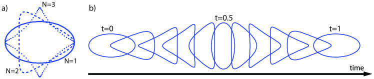
Figure 3.1: The relationship between the conformal mapping and the shape of the swimmer: a): Shapes determined by $w(\zeta)=4\zeta+\zeta^{-N}$, where $N=1$ (solid line, ellipse), $N=2$ (dashed line, triangle), or $N=3$ (dotted line, quadrilateral). b): A sequence of shape changes defined by $w(\zeta;t)=3\zeta+\cos(2\pi t)\zeta^{-1}-\sin(2\pi t)\zeta^{-2}$.

We assume that the boundary condition is in the general form of $V(\sigma;t)=\sum\lambda_{n}(t)\sigma^{n}$, and we first prove the following result in some particular cases.

Lemma 2

Suppose that the conformal mapping $w(\zeta)$ is given by (3.1) and the boundary condition is given as $V(\sigma)=\sum\lambda_{n}\sigma^{n}$. Let $-V^{+}(\zeta)$ be the analytic part of $V(\zeta)$ when $|\zeta|>1$, which has the form $-V^{+}(\sigma;t)=\sum_{n\leq 0}\lambda_{n}(t)\sigma^{n}$. If there exists a function $f_{N}(\zeta)$ analytic on $|\zeta|<1$, continuous on $|\zeta|\leq 1$, and

$$f_{N}(\sigma)\Big{|}_{\sigma\in S^{1}}=\sigma^{N}\dfrac{w(\sigma)}{\overline{w^{\prime}(\sigma)}}$$

for some $N\in\mathbb{Z}^{+}$, $N\geq 2$, then for any $-V^{+}(\zeta)$ with Laurent series such that $\lambda_{-1}=\lambda_{-2}=\cdots=\lambda_{-(N-2)}=0$ for $N>2$ (if $N=2$ there are no restrictions on the coefficients), the solution to the boundary value problem (2.20) is given by

$$\Phi(\zeta) = -V^{+}(\zeta)$$

$$\Psi(\zeta) = \dfrac{\overline{w}(1/\zeta)}{w^{\prime}(\zeta)}V^{+^{\prime}}(\zeta)-\overline{V^{-}}(1/\zeta)$$

for $|\zeta|\geq 1$.

Lemma 2 can be proved by direct calculation as follows.

Proof

The function $-V^{+}$ has the representation

$$-V^{+}(\zeta)=\dfrac{\lambda_{-(N-1)}}{\zeta^{N-1}}+\dfrac{\lambda_{-N}}{\zeta^{N}}+\cdots+\dfrac{\lambda_{-n}}{\zeta^{n}}+\cdots$$

Suppose that $\Phi(\zeta)=-V^{+}(\zeta)$. Then on the unit circle $S^{1}$, we have

$$\overline{\Phi^{\prime}(\sigma)}=-\sigma^{N}\big{[}\big{(}N-1\big{)}\overline{\lambda_{-(N-1)}}+N\overline{\lambda_{-N}}\sigma+\cdots+n\overline{\lambda_{-n}}\sigma^{n-N+1}+\cdots\big{]}$$

and the integral term in (2.24) becomes

$$\dfrac{1}{2\pi i}\int_{S^{1}}\dfrac{w(\sigma)}{\overline{w^{\prime}(\sigma)}}\dfrac{\overline{\Phi^{\prime}(\sigma)}}{\sigma-\zeta}d\sigma$$

$$= -\dfrac{1}{2\pi i}\int_{S^{1}}\dfrac{f_{N}(\sigma)}{\sigma-\zeta}\big{[}\big{(}N-1\big{)}\overline{\lambda_{-(N-1)}}+N\overline{\lambda_{-N}}\sigma+\cdots+n\overline{\lambda_{-n}}\sigma^{n-N+1}+\cdots\big{]}d\sigma.$$

Since the function

$$g(\sigma)=f_{N}(\sigma)[(N-1)\overline{\lambda_{-(N-1)}}+N\overline{\lambda_{-N}}\sigma+\cdots+n\overline{\lambda_{-n}}\sigma^{n-N+1}+\cdots]$$

is analytic on $|\sigma|<1$ and continuous on $|\sigma|\leq 1$, and since $|\zeta|>1$, the integral

$$\dfrac{1}{2\pi i}\int_{S^{1}}\dfrac{g(\sigma)}{\sigma-\zeta}d\sigma=0$$

by the Cauchy Integral Theorem. Hence the left hand side of (2.24) reduces to $\Phi(\zeta)=-V^{+}(\zeta)$. By substituting this result into (2.20), we obtain the expression of $\Psi$ as in the lemma. Q.E.D.

With $w$ given by (3.1) we have

$$\genfrac{}{}{}{}{w(\sigma)}{\raisebox{-3.0pt}{$\overline{w^{\prime}(\sigma)}$}}=\genfrac{}{}{}{}{\alpha_{1}\sigma+\alpha_{0}+\alpha_{-1}\sigma^{-1}+\alpha_{-2}\sigma^{-2}+\cdots+\alpha_{-N}\sigma^{-N}}{\raisebox{-3.0pt}{$\overline{\alpha_{1}}-\overline{\alpha_{-1}}\sigma^{2}-2\overline{\alpha_{-2}}\sigma^{3}-\cdots-N\overline{\alpha_{-N}}\sigma^{N+1}$}}$$

hence we may take

$$f_{N}(\zeta) = \zeta^{N}\genfrac{}{}{}{}{\alpha_{1}\zeta+\alpha_{0}+\alpha_{-1}\zeta^{-1}+\alpha_{-2}\zeta^{-2}+\cdots+\alpha_{-N}\zeta^{-N}}{\raisebox{-3.0pt}{$\vspace*{3pt}\overline{\alpha_{1}}-\overline{\alpha_{-1}}\zeta^{2}-2\overline{\alpha_{-2}}\zeta^{3}-N\overline{\alpha_{-N}}\zeta^{N+1}$}}$$ (3.2)

$$= \genfrac{}{}{}{}{\alpha_{-N}+\alpha_{-(N-1)}\zeta+\cdots+\alpha_{-1}\zeta^{N-1}+\alpha_{0}\zeta^{N}+\alpha_{1}\zeta^{N+1}}{\raisebox{-3.0pt}{$\overline{\alpha_{1}}-\overline{\alpha_{-1}}\zeta^{2}-2\overline{\alpha_{-2}}\zeta^{3}-\cdots-N\overline{\alpha_{-N}}\zeta^{N+1}$}}$$

If no singularity of $f_{N}$ lies inside the unit disk $|\zeta|<1$, then $f_{N}$ is analytic on $|\zeta|<1$ and we may apply Lemma 2 to obtain the solution of the boundary condition constraint (2.14).

The Laurent expansion of any function $\Phi(\zeta)$ that is analytic on $|\zeta|>1$, continuous on $|\zeta|=1$, has the form of  (2.17). Let $\mathcal{S}$ be the set

$$\mathcal{S}=\Big{\{}\Phi(\zeta)=\dfrac{A_{-1}}{\zeta}+\dfrac{A_{-2}}{\zeta^{2}}+\dfrac{A_{-3}}{\zeta^{3}}+\cdots;\sum_{k\geq 1}k|A_{-k}|<+\infty\Big{\}}$$

of all functions $\Phi(\zeta)$ whose coefficients of the Laurent expansion satisfy $\sum_{k\geq 1}k|A_{-k}|<+\infty$ and vanish at infinity. $\mathcal{S}$ is a Banach space endowed with the norm $\parallel\Phi\parallel=\sum_{k\geq 1}k|A_{-k}|$ (Chambrion & Munnier, 2011).

Now with $w$ given by (3.1), we define a conjugate linear operator $\bm{K}(w)$ on $\mathcal{S}$ as

$$\big{[}\bm{K}(w)\circ\Phi\big{]}(\zeta)=\dfrac{1}{2\pi i}\int_{S^{1}}\dfrac{w(\sigma)}{\overline{w^{\prime}(\sigma)}}\dfrac{\overline{\Phi^{\prime}(\sigma)}}{\sigma-\zeta}d\sigma$$ (3.3)

Let $\mathcal{S}_{0}=\{A_{0}\in\mathbb{C}\}$, then $\bm{K}(w)$ can be extended to $\mathcal{S}\oplus\mathcal{S}_{0}$ such that $\bm{K}(w)|_{\mathcal{S}_{0}}\equiv 0$ in accordance with (3.3). Now for any $\Phi\in\mathcal{S}\oplus\mathcal{S}_{0}$, (2.24) can be written as

$$\big{[}\bm{I}+\bm{K}(w)\big{]}\Phi=-V^{+}$$

where $\bm{I}$ is the identity operator. For $n\in\mathbb{Z}^{+}$, let

$$\mathcal{S}_{n}^{\Re}=\big{\{}\dfrac{r}{\zeta^{n}};r\in\mathbb{R}\big{\}}\qquad\textrm{and}\qquad\mathcal{S}_{n}^{\Im}=\big{\{}\dfrac{ir}{\zeta^{n}};r\in\mathbb{R}\big{\}}$$

It is easily seen that $\mathcal{S}_{n}^{\Re}$’s and $\mathcal{S}_{n}^{\Im}$’s are real $1$-dimensional linear subspaces of $\mathcal{S}$. With $f_{N}$ given by (3.2), by Lemma 2, $\bm{K}(w)$ vanishes on each $\mathcal{S}_{n}^{\Re}$ and $\mathcal{S}_{n}^{\Im}$ for $n=N-1,N,N+1,\cdots$, and thus each $\mathcal{S}_{n}^{\Re}$ or $\mathcal{S}_{n}^{\Im}$ is invariant under the operator $\bm{I+K}(w)$, i.e.,

$$\big{[}\bm{I}+\bm{K}(w)\big{]}\big{|}_{\mathcal{S}_{n}^{\Re}}=\bm{I}_{\mathcal{S}_{n}^{\Re}};\qquad\qquad\big{[}\bm{I}+\bm{K}(w)\big{]}\big{|}_{\mathcal{S}_{n}^{\Im}}=\bm{I}_{\mathcal{S}_{n}^{\Im}}$$

Define

$$\mathcal{S}_{N}:=\textrm{Span}_{\mathbb{R}}\{\zeta^{-n},i\zeta^{-n}\}_{n=-1}^{-(N-2)}=\bigoplus_{n=-1}^{-(N-2)}\big{(}\mathcal{S}_{n}^{\Re}\bigoplus\mathcal{S}_{n}^{\Im}\big{)}$$

which is a real $2(N-2)$-dimensional linear subspace of $\mathcal{S}$, and

$$\{\zeta^{-1},\zeta^{-2},\cdots,\zeta^{N-2},i\zeta^{-1},i\zeta^{-2},\cdots,i\zeta^{N-2}\}$$

consists a basis of $\mathcal{S}_{N}$. If $f_{N}$ is analytic on $|\zeta|<1$, then the action of $\bm{K}(w)$ on this basis can be expressed as

$$\big{[}\bm{K}(w)\big{]}\circ\zeta^{-n} = -\dfrac{n}{2\pi i}\int_{S^{1}}\dfrac{f_{N}(\sigma)}{\sigma-\zeta}\dfrac{1}{\sigma^{N-n-1}}d\sigma=\dfrac{n}{\zeta^{N-n-1}}\sum_{k=0}^{N-n-2}\dfrac{f_{N}^{(k)}(0)}{k!}\zeta^{k}$$

$$\big{[}\bm{K}(w)\big{]}\circ\big{(}i\zeta^{-n}\big{)} = \dfrac{n}{2\pi}\int_{S^{1}}\dfrac{f_{N}(\sigma)}{\sigma-\zeta}\dfrac{1}{\sigma^{N-n-1}}d\sigma=-\dfrac{in}{\zeta^{N-n-1}}\sum_{k=0}^{N-n-2}\dfrac{f_{N}^{(k)}(0)}{k!}\zeta^{k}$$

for $n=1,2,\cdots,N-2$. Notice that the sum in the above equations is simply the first $N-n-1$ terms of the Laurent expansion of $f_{N}(\zeta)$ at $\zeta=0$. It is easily seen that on $\mathcal{S}_{N}$, the operator $\bm{K}(w)$ has a matrix representation as

$$\big{[}\bm{K}(w)\big{]}\circ(\zeta^{-1},\zeta^{-2},\cdots,\zeta^{-(N-2)})^{T} = K(w)\cdot(\zeta^{-1},\zeta^{-2},\cdots,\zeta^{-(N-2)})^{T}$$

$$\big{[}\bm{K}(w)\big{]}\circ(i\zeta^{-1},i\zeta^{-2},\cdots,i\zeta^{-(N-2)})^{T} = -K(w)\cdot(i\zeta^{-1},i\zeta^{-2},\cdots,i\zeta^{-(N-2)})^{T}$$

where $K(w)$ is a $(N-2)\times(N-2)$ matrix with the form

$$K(w)=\left(\begin{array}[]{cccccccc}\dfrac{f_{N}^{(N-3)}(0)}{(N-3)!}&\dfrac{f_{N}^{(N-4)}(0)}{(N-4)!}&\cdots&\cdots&\cdots&\dfrac{f_{N}^{\prime\prime}(0)}{2!}&\dfrac{f_{N}^{\prime}(0)}{1!}&\dfrac{f_{N}(0)}{0!}\\ \dfrac{2f_{N}^{(N-4)}(0)}{(N-4)!}&\dfrac{2f_{N}^{(N-5)}(0)}{(N-5)!}&\cdots&\cdots&\cdots&\dfrac{2f_{N}^{\prime}(0)}{1!}&\dfrac{2f_{N}(0)}{0!}&0\\ \dfrac{3f_{N}^{(N-5)}(0)}{(N-5)!}&\dfrac{3f_{N}^{(N-6)}(0)}{(N-6)!}&\cdots&\cdots&\cdots&\dfrac{3f_{N}(0)}{0!}&0&0\\ \vdots&\vdots&&&\cdotp&0&0&\vdots\\ \vdots&\vdots&&\cdotp&\cdotp&\vdots&\vdots&\vdots\\ \vdots&\vdots&\cdotp&\cdotp&&\vdots&\vdots&\vdots\\ \dfrac{(N-3)f_{N}^{\prime}(0)}{1!}&\dfrac{(N-3)f_{N}(0)}{0!}&0&\cdots&\cdots&0&0&0\\ \dfrac{(N-2)f_{N}(0)}{0!}&0&\cdots&\cdots&\cdots&0&0&0\\ \end{array}\right)$$ (3.12)

This can be summarized as follows.

Lemma 3

Suppose that the conformal mapping $w(\zeta)$ is given by (3.1) and the boundary condition is given as $V(\sigma)=\sum\lambda_{n}\sigma^{n}$. If there exists a function $f_{N}(\zeta)$ analytic on $|\zeta|<1$, continuous on $|\zeta|\leq 1$, and

$$f_{N}(\sigma)\Big{|}_{\sigma\in S^{1}}=\sigma^{N}\dfrac{w(\sigma)}{\overline{w^{\prime}(\sigma)}}$$

for some $N\in\mathbb{Z}^{+}$, $N\geq 2$, then the integral (2.24) reduces to linear relations between coefficients of $\Phi$ and $V$:

1. For $n=0$ or $n\geq N-1$, $A_{-n}=\lambda_{-n}$;

2. For $1\leq n\leq N-2$:

   $$\big{(}I_{N-2}+K(w)\big{)}\big{(}\Re A_{-1},\cdots,\Re A_{-(N-2)}\big{)}^{T} = \big{(}\Re\lambda_{-1},\cdots,\Re\lambda_{N-2}\big{)}^{T}$$

   $$\big{(}I_{N-2}-K(w)\big{)}\big{(}\Im A_{-1},\cdots,\Im A_{-(N-2)}\big{)}^{T} = \big{(}\Im\lambda_{-1},\cdots,\Im\lambda_{N-2}\big{)}^{T}$$

   where $I_{N-2}$ is the $(N-2)$-identity matrix, and $K(w)$ is the $(N-2)\times(N-2)$ matrix given by (3.12).

Lemma 3 provides an algorithm for solving the Stokes equation of an infinite $2$D Stokes flow when the shape deformations have finitely many terms in the conformal mapping $w(\zeta)$. Once we solve for $\Phi$ according to Lemma 3, $\Psi$ is given by the following expression.

$$\Psi(\zeta;t) = -\dfrac{\overline{\dot{\alpha}_{1}}}{\zeta}+\overline{\big{(}A_{-1}-\dot{\alpha}_{-1}\big{)}}\zeta+\overline{\big{(}A_{-2}-\dot{\alpha}_{-2}\big{)}}\zeta^{2}+\cdots+\overline{\big{(}A_{-N}-\dot{\alpha}_{-N}\big{)}}\zeta^{N}$$ (3.13)

$$\genfrac{}{}{}{}{\dfrac{\overline{\alpha_{1}}}{\zeta}+\overline{\alpha_{-1}}\zeta+\overline{\alpha_{-2}}\zeta^{2}+\cdots+\overline{\alpha_{-N}}\zeta^{N}}{\raisebox{-6.0pt}{$\alpha_{1}-\dfrac{\alpha_{-1}}{\zeta^{2}}-\dfrac{2\alpha_{-2}}{\zeta^{3}}-\cdots-\dfrac{N\alpha_{-N}}{\zeta^{N+1}}$}}\Big{(}\dfrac{A_{-1}}{\zeta^{2}}+\dfrac{2A_{-2}}{\zeta^{3}}+\cdots+\dfrac{NA_{-N}}{\zeta^{N+1}}\Big{)}\quad$$

4 Modeling of swimming Dictyostelium amoebae

As mentioned in the Introduction, Dictyostelium amoebae can move in a fluid environment by a combination of blebbing and protrusions, either of which involve rapid shape changes and neither of which require attachment to a substrate. Experimental observations on the movement of Dd cells reported in Barry & Bretscher, (2010), Bae & Bodenschatz, (2010) and Van Haastert, (2011) have recorded cell shape changes, speeds, and periods of the cyclic motion, and we use their data here to compare with theoretical predictions. The movement usually involves protrusions that are initiated at the leading edge of the cell and which propagate toward the rear. Typically the cell body is elongated, and multiple protrusions propagate along the cell. van Haastert (Van Haastert, 2011) reported an average of three protrusions, as illustrated by the cartoon model in Figure 4.1 (a), while from the experimental images (Figure 4.1 (b)) of a swimming Dictyostelium reported in Barry et.al. (Barry & Bretscher, 2010), we see that one protrusion travels along one side of the cell and disappears at the rear of the cell, then another protrusion appears on the other side and repeats the process.

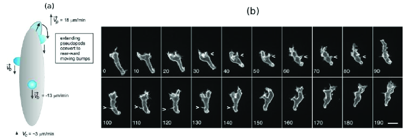
Figure 4.1: Amoebae swim by protrusions: (a) a swimming cell with $3$ protrusions (Van Haastert, 2011); (b) the shape of an amoeboid as it swims (Barry & Bretscher, 2010).

Van Haastert (Van Haastert, 2011) observed that the protrusions travel directly down the cell body and not in a helical fashion. Thus there is no clear evidence that the cell is rotating around its symmetry axis, and as a result we consider the 2D model developed in the preceding sections to be a reasonable simplification of a 3D swimming cell. In Section 4.1 the numerical scheme used to construct the shape of the cell is developed. As we see from Figure 4.1, swimming by extending protrusions is mostly asymmetric in that they alternate sides, and thus the motion is not rotation-free and the trajectory of a swimming cell is snake-like rather than along a straight line. However we begin in Section 4.2 with a simplified symmetric amoeba, where a pair of side protrusions move down the cell body symmetrically so as to minimize the mechanical effects resulted from rotation or cell body twisting. In Section 4.3 we investigate how different cell and protrusion shapes affect the swimming ability of such a translational swimmer. Finally, in Section 4.4 we consider an asymmetric swimmer similar to that shown in Figure 4.1(b) and compare such a snake-like swimming style to the symmetric swimming style.

4.1 Construction of the cell shape

To apply the Muskhelishvili method to a swimming cell we first have to obtain the conformal mapping $w$ corresponding to the cell shape, and then truncate its Laurent’s expansion, leaving only $N$ negative order terms for some $N$. In general it is difficult to find the conformal mapping analytically that corresponds to a general shape, yet that of an $n$-polygon can be found by use of the Schwarz-Christoffel formula (Ahlfors, 1978, Driscoll & Trefethen, 2002).

Suppose that we have an $n$-polygon in the $z$-plane with vertices $z_{1},\cdots,z_{n}$, and the corresponding exterior angles are $\theta_{1}\pi,\cdots,\theta_{n}\pi$ (Figure 4.2). Let $\Omega$ be the interior region

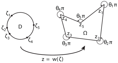
Figure 4.2: The conformal mapping for the exterior region of a polygon from that of the unit disk.

bounded by the polygon. The conformal mapping from the exterior of the unit disk $D$ in the $\zeta$-plane to $\Omega^{c}$ is given by the following Schwarz-Christoffel (SC) formula (Ahlfors, 1978, Driscoll & Trefethen, 2002):

$$z=w(\zeta)=A+C\int^{\zeta}\dfrac{1}{\xi^{2}}\prod_{k=1}^{n}\big{(}\xi-\zeta_{k}\big{)}^{\theta_{k}-1}d\xi$$ (4.1)

where $z_{k}=w(\zeta_{k})$ and we call $\zeta_{k}$ the prevertex to the vertex $z_{k}$ under the conformal mapping $z=w(\zeta)$. Since we are considering transformation from the exterior region of $D$ to the exterior region of $\Omega$, the angles should satisfy $\sum_{k=1}^{n}\theta_{k}=n+2$. The prevertices $\zeta_{k}$ can be numerically approached by using the SC toolbox given at http://www.math.udel.edu/~driscoll/SC/. Once we have obtained the Schwarz-Christoffel transformation $w_{\textrm{SC}}(\zeta)$ for a given polygon, we truncate its Laurent expansion leaving only $N$ negative order terms, which then has the form

$$w_{\textrm{SCN}}(\zeta)=\alpha_{1}\zeta+\alpha_{0}+\dfrac{\alpha_{-1}}{\zeta}+\cdots+\dfrac{\alpha_{-N}}{\zeta^{N}}.$$ (4.2)

The image of the unit circle $S^{1}$ under the truncated conformal mapping $w_{\textrm{SCN}}$ is a contour approximating the original polygon.

We approach the construction of the shape of a swimming amoeba as follows. Instead of using a polygonal discretization with many nodes on the boundary, we first construct an ”inner skeleton” of the cell with only a few nodes (Figure 4.3, red contours), then we obtain its

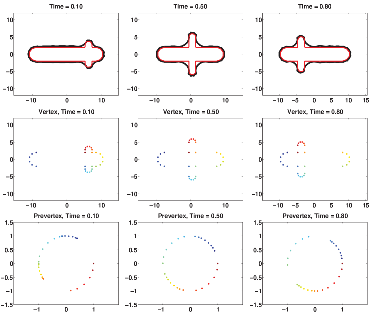
Figure 4.3: The conformal mapping for the exterior region of a polygon from that of the unit disk. The axes are in units of $\mu m$.

Schwarz-Christoffel transformation and truncate it to obtain $w_{\textrm{SCN}}$. Finally we smooth the image of the unit circle under $w_{\textrm{SCN}}$ by multiplying the amplitude of $\alpha_{1}$ in (4.2) by a factor $C\in\mathbb{R}$, $C>1$, to give

$$w_{N}(\zeta)=C\alpha_{1}\zeta+\alpha_{0}+\dfrac{\alpha_{-1}}{\zeta}+\cdots+\dfrac{\alpha_{-N}}{\zeta^{N}}.$$ (4.3)

This will give us a smoothed contour enclosing the ”inner skeleton”, and we use it as the shape of cell (Figure 4.3, black contours). Figure 4.3 illustrates this process, and the detailed steps of the algorithm are given in the appendix C. The panels in the top row give three snapshots within one cycle. The red contours give the ”inner skeletons”, each one is a prescribed polygon, with each of the four semicircle ends having five nodes. The black contours that are taken as the current cell shapes, are determined by a conformal mapping of the form of (4.2) with $N=30$ and $C=1.05$. The panels in the middle and bottom rows show the distribution of vertices of the polygon ($z_{i}$ in Figure 4.2) and the distribution of prevertices along the unit circle ($\zeta_{i}$ in Figure 4.2), with the correspondence relation given by the color of the dots. From Figure 4.3 we see that when the two side protrusions are close to either end of the cell body, some prevertices are crowded and when the side protrusions are near the middle of the cell body, the prevertices are more scattered.

In the simulations described later we do not require strict area conservation – instead we require that the area changes be restricted within a small range. We define the ratio of area change within one period to be

$$\textrm{Ratio of area change}=\dfrac{\textrm{Maximum of area}-\textrm{Minimum of area}}{\textrm{Average of area}}$$

and we require that the ratio be $\leq 0.1$.

4.2 Simulation results of swimming Dictyostelium amoebae

We use the data for swimming amoebae from (Van Haastert, 2011, Barry & Bretscher, 2010). Though they are both Dictyostelium amoebae, they have different sizes. For simplicity we will refer to them as “van Haastert’s cell” (Figure 4.1 (a)) and “Barry’s cell” (Figure 4.1 (b)) hereafter. Their data is shown in Table 3.

Table 3: Experimental data for Van Haastert’s cell (Van Haastert, 2011) and Barry’s cell (Barry & Bretscher, 2010).

Van Haastert Barry Maximum cell body length $\sim 25\mu m$ $\sim 22\mu m$ Average cell body width $\sim 6\mu m$ $\sim 4\mu m$ Maximum protrusion height $\sim 2\mu m$ $\sim 4\mu m$ Average protrusion width $\sim 2\mu m$ $\sim 2\mu m$ Period of a stroke $\sim 1\textrm{min}$ $\sim 1.5\textrm{min}$

We use the numerical methods discussed in Section 4.1 to generate sequences of shapes based on data given in Table 3. The numerical results are presented in Figure 4.4. The shapes of Barry’s cell within a cycle for different values of $N$ are shown in Figure 4.4(a-c), while those of van Haastert’s cell are shown in Figure 4.4(d-f). Figure 4.4(g-i) compare the mean velocity $\widetilde{U}$, mean power $\overline{\mathcal{P}}$ and performance $E$ of the two cells for $N\in[10,80]$.

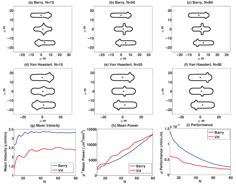
Figure 4.4: (a-c) The shapes of Barry’s cell within a cycle for different values of $N$. (d-f) The shapes of van Haastert’s cell within a cycle for different values of $N$. In (a-f), the top rows are the snapshots at the beginning of a cycle, the middle rows are at half of the cycle, and the bottom rows are at the end of the cycle. For the periods of the two cells, we have $T_{B}=1.5\ \textrm{min}$ for Barry’s cell and $T_{H}=1\ \textrm{min}$ for van Haastert’s cell. (g-i) A comparison of the mean velocity $\widetilde{U}$, mean power $\widetilde{\mathcal{P}}$ and performance $E$ of the two cells for $N\in[10,80]$.

A number of conclusions can be drawn from these simulations, as listed below.

1. Protrusion shape. First we consider how the number of terms $N$ in the conformal mappings $w_{N}$ affects the shapes of the swimmers. As we mentioned earlier, in general the $\zeta^{-n}$ term gives $n$ angles along the periphery of the cell. From Figure 4.4(a - f) we see that swimmers corresponding to $w_{N}$ with larger $N$ have more rounded heads in the protrusions, while those corresponding to $w_{N}$ with smaller $N$ tend to have sharper heads; another important difference in the shapes of the protrusions is that the connecting parts between the cell body and the protrusions are smoother for smaller $N$ while more abrupt for larger $N$. Figure 4.5 gives an enlarged view of the protrusion regions of both cells with different $N$.

   

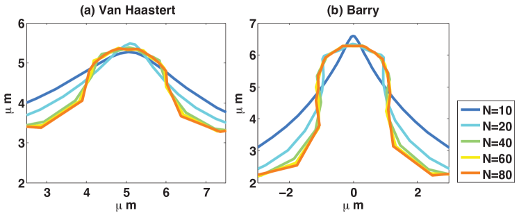
   Figure 4.5: The areas of the protrusions in the models of van Haastert’s and Barry’s cells for different $N$: (a)van Haastert’s cell; (b) Barry’s cell.

2. Velocity. For either cell, the mean velocity $\widetilde{U}$ increases rapidly with $N$ when $N$ is small, but $\widetilde{U}$ does not change much for even larger $N>\sim 40$ (Figure 4.4(g)). For $N\geq 40$, $\widetilde{U}$ of van Haastert’s cell fluctuates within a range $2.37-2.52\mu m/\textrm{min}$ while $\sim 3.30\mu m/\textrm{min}$ for Barry’s cell. Taking into account of our observation of the relation between $N$ and protrusion shapes, our simulation results indicate that abrupt protrusions with rounded heads may enhance the swimming speed.

3. Power. Unlike the mean velocity $\widetilde{U}$ which has a maximum as $N$ increases, the mean power $\overline{\mathcal{P}}$ continues increasing as $N$ increases (Figure 4.4(h)). In particular, if we observe Figures 4.4(b,c,e,f), we see that the shapes of the same cell for $N=50$ and $N=80$ are quite similar, yet with more terms in $w_{N}$ it requires much more power.

4. Performance. Figure 4.4(i) clearly shows that performance decreases as more terms $N$ in $w_{N}$ are involved. Incorporating the observation of bump shapes, we find that smoother protrusions tend to lead to swimming with better performance though it might be slower.

5. Comparing with experimental data. van Haastert (Van Haastert, 2011) reported that the swimming velocity of a typical cell is $\sim~{}3\mu m/\textrm{min}$, while our model predicts $\sim 1.36-2.52~{}\mu m/\textrm{min}$. Barry at.el. (Barry & Bretscher, 2010) reported that the linear speed of the cells has a range of $2-8.4~{}\mu m/\textrm{min}$ with an average of about $4.2\mu m/\textrm{min}$, comparing to a range of $\sim 2.63-3.31\mu m/\textrm{min}$ as given by our numerical simulations. So far there are no experimental data regarding the power or performance of the swimming amoebae, and based on the data of swimming speed collected from experiments, we believe our model is reasonable.

6. How cell shapes affect the swimming behavior. Both cells are the same kind of Dictyostelium amoebae, but from the above results and observations we clearly see that different cell shapes and sizes lead to the difference in their swimming behavior: as compared with van Haastert’s cell, Barry’s cell is more slender, with higher protrusions, and smaller in size, and the simulation results show that the average area for van Haastert’s cell ranges within $170\mu m^{2}-174\mu m^{2}$, depending on the value of $N$, while the average area for Barry’s cell is only within $103\mu m^{2}-106\mu m^{2}$. Figure 4.4 indicates that Barry’s cell exhibits faster swimming and better performance. This inspires us to study how the sizes of the cell body and the protrusions affect the swimming behavior of the cell, which will be discussed in detail in the following section.

4.3 Effects of the protrusion height and cell body shapes on swimming

We first study the effects of the protrusion shape on the swimming behavior of the Dictyostelium amoebae. As above we use the data for the sizes of different characteristic features of a cell in Van Haastert, (2011) and Barry & Bretscher, (2010), which are presented in Table 3. As for the conformal mappings, we truncate them at $N=30$ so as to generate protrusions that are neither too smooth nor too abrupt. At each time step we adjust the cell body length to compensate for the area changes caused by the emergence and disappearance of the protrusions, so as to control the area change of the whole cell within a small range. We test for different maximum protrusion heights, ranging from $1.5\mu m-5\mu m$. Figure 4.6 gives the relationship between the mean velocity, mean power, and performance and the maximum protrusion height for both Barry’s and van Haastert’s cells. First we see that the mean velocity increases significantly as the protrusion becomes taller (Figure 4.6 (a)). On the other hand the mean power for Barry’s cell increases steadily as the protrusion height increases, while for van Haastert’s cell the mean power first increases but for taller protrusions it approaches a maximum (Figure 4.6 (b)). Finally for the performance, it turns out that Barry’s cell,which is smaller, always performs better than van Haastert’s cell, though it swims slower than van Haastert’s (Figure 4.6 (c)). Moreover, while the performance for van Haastert’s cell increases as the protrusion grows higher, the protrusion height does not have much effect on the performance of Barry’s cell.

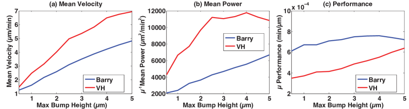
Figure 4.6: Effects of the protrusion height on swimming for van Haastert’s and Barry’s cell: (a): mean velocity $\sim$ maximum protrusion height; (b): mean power $\sim$ maximum protrusion height; (c): performance $\sim$ maximum protrusion height.

Next we consider the effects of the cell body shape on the swimming behaviors of Dictyostelium amoebae by varying the length to width ratio of cells. We consider protrusions with the same height ($\sim 3\mu m$) and width ($\sim 2\mu m$) and let the shape deformations have the same period ($=1\textrm{min}$). Moreover, to reduce the computational effort we keep the protrusion height constant through the whole cycle, ie, we do not consider the emergence, growth and disappearance processes of the protrusions as in previous simulations that led to Figure 4.6. To make the comparison fair, we control the average area of each cell within a certain range ($\sim 176\mu m^{2}-205\mu m^{2}$).

We define the aspect ratio $R_{s}$ of the cells as

$$R_{s}=\dfrac{\textrm{Cell body length}}{\textrm{Cell body width}}$$

so that large (small) $R_{s}$ corresponds to slender (rounded) bodies. The relations of mean velocity, mean power and performance to the ratio of the cell body sizes $R_{s}$ are given in Figure 4.7, from which we see that slender cells swim faster than rounded ones (Figure 4.7(a)), yet they require more power expenditure (Figure 4.7(b)) and the performance is worse (Figure 4.7(c)). We should note that although in general Barry’s cell is more slender than van Haastert’s cell, yet Barry’s cell is much more smaller, thus it swims more slowly, yet with better performance (Figure 4.6).

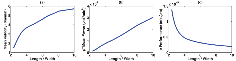
Figure 4.7: Effects of the cell body shape on swimming: (a): mean velocity $\sim$ $R_{s}$; (b): mean power $\sim$ $R_{s}$; (c): performance $\sim$ $R_{s}$.

Based on our observations on the protrusion height and the cell’s slenderness, we conclude that

1. Within a reasonable range, protrusions with large height will result in faster swimming and better performance.

2. Slender cells swim faster, but their performance is worse than those rounded ones.

4.4 Do asymmetric shape deformations improve swimming?

In Sections $\ref{Ddsim}-\ref{Height}$ we discussed symmetric shape deformations for amoebae swimming at LRN, but to date there is no clear evidence which shows that amoebae favor such symmetric modes . Rather, they seem to prefer asymmetric modes in which the protrusions travel one by one (Figure 4.1) (Van Haastert, 2011, Barry & Bretscher, 2010). In the 2D model of swimming (Figure 4.1(b)) this means that the protrusions at the two sides alternate rather than appearing symmetrically, so that the cell swims in a snake-like trajectory. This raises the question as to why amoebae employ the asymmetric mode – are there advantages over the symmetric mode or are protrusions constrained by the internal dynamics?

We design an asymmetric swimmer for which the protrusions alternate sides during successive cycles, and adapt the previous numerical scheme. Asymmetric swimmers are not rotation-free, hence we must consider the torque on the swimmer, and the rotational velocity is calculated via (2.27) (Figure 4.8, center). We compare the asymmetric swimmer with two symmetric swimmers whose cell body and protrusion shapes are identical, and whose conformal mapping is truncated at the same order $N$. One of them propagates its pair of protrusions at the same speed as the asymmetric swimmer (Figure 4.8, top), while the other propagates its pair of protrusions at half the speed of the others (Figure 4.8, bottom).

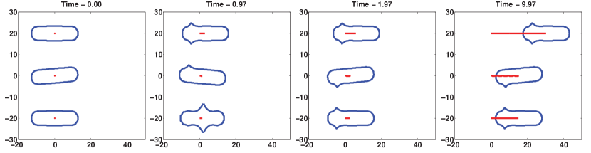
Figure 4.8: A comparison of the three swimming amoebae. The top and bottom rows use the same sequence of shape changes, but protrusions in the bottom row travel at half the speed of those in the top row. The asymmetric swimmer in the center row alternates the protrusions on the two sides. The period for the symmetric swimmers is 1 min, while for the asymmetric swimmer it is 2 min. The axes are in units of $\mu m$.

The red lines in Figure 4.8 reflect the trajectories of the center of mass of each swimmer, and one sees that both symmetric swimmers move in a straight line (i.e., rotation-free) while the asymmetric swimmer in the center images swims in a slightly snake-like style. The simulations show that the symmetric swimmer propagating its pair of protrusions at the same speed (Figure 4.8, above) as the asymmetric swimmer travels a distance of $X\sim 30.33$ for $T=10$, while the asymmetric swimmer travels a distance of $X\sim 15.36$ in the same time, which is slightly more than half the distance traveled by the symmetric swimmer and slightly more than that for the symmetric swimmer in (Figure 4.8, below). The average power of the asymmetric swimmer is again almost half that of the symmetric one with the same protrusion speed, hence their performance is the same. Thus we find that rotation that results from the asymmetric shape deformations does not lead to a reduction of performance, since the swimmer expends half the energy in swimming half as fast.

Finally we show that when a protrusion always moves along one side, the cell simply rotates in the long run. In this case the global trajectory of the center of mass is a circle generated after a sufficient number of cycles (Figure 4.9).

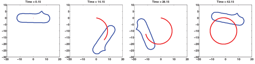
Figure 4.9: The rotating amoeba. Lengths are measured in microns.

5 Discussion

Movement of eukaryotic cells is best-characterized for keratocytes, which use actin-driven lamellipodia at the leading and myosin-driven contraction at the rear to move (Keren & Theriot, 2008). They move with very little shape change, which simplifies their description, and several models that reproduce the shape have been proposed(Herant & Dembo, 2010, Rubinstein et al., 2009, Wolgemuth et al., 2011). Understanding of the mechanical balances that produce stable gliding motion is emerging, but the linkage between the biochemical state and the mechanical state is still not understood. For example, how an initially symmetric cell breaks the symmetry of the rest state and begins to move, and how the localization of the control molecules and the properties of substrate affect motion, has not been explained.

In contrast, other cells are found to use very complicated shape changes for locomotion, and this has led to the overarching question posed by experimentalists, which is ‘How does deformation of the cell body translate into locomotion?’(Renkawitz & Sixt, 2010). The model and results described herein on swimming by shape changes was motivated by recent experiments which show that both neutrophils and Dd can swim – in the strict sense of propelling themselves through a fluid without using any attachments – in response to chemotactic gradients. Our results for 2D cells show how the shape and height of a protrusion affect the speed and efficiency of swimming and may give insights into optimal designs of micro-robots.

The protrusions and other shape changes used in swimming require forces that must be correctly orchestrated in space and time to produce net motion, and to understand this orchestration one must couple the cellular dynamics with the dynamics of the surrounding fluid or ECM. This remains an open problem for future research.

Appendix A Translation of the swimmer: proof of (2.26)

Proof

$U_{\infty}$ is defined as the translation part of the velocity field at infinity (Shapere & Wilczek, 1989b ),

$$U_{\infty}=\lim_{R\rightarrow\infty}\oint\dfrac{d\theta}{2\pi}u$$

where $u$ is the fluid velocity field in the exterior domain. In 2D it can be expressed by the complex integral

$$U_{\infty}=\lim_{R\rightarrow\infty}\dfrac{1}{2\pi i}\oint_{|z|=R}\dfrac{u(z,\overline{z})}{z}dz$$ (A.1)

Choose $R>0$ large enough so that $\phi$ and $\chi^{\prime}$ are analytic on $|z|>R$ and continuous on $|z|\geq R$. Let $\xi=z/R$ and then by (A.1) and Table 1,

$$U_{\infty}=\lim_{R\rightarrow\infty}\dfrac{1}{2\pi i}\oint_{|\xi|=1}\Big{[}\dfrac{\phi(R\xi)}{\xi}-R\overline{\phi^{\prime}(R\xi)}-\dfrac{\overline{\chi^{\prime}(R\xi)}}{\xi}\Big{]}d\xi.$$ (A.2)

Let

$$\widetilde{\phi}(\xi)=\phi^{\prime}(R\xi),\qquad\widetilde{\psi}(\xi)=\chi^{\prime}(R\xi)$$

Obviously, $\widetilde{\phi}$, $\widetilde{\psi}$ are analytic on $|\xi|>1$ (including at infinity) and continuous on $|\xi|\geq 1$. Define

$$\overline{\widetilde{\phi}}(\xi)=\overline{\widetilde{\phi}(\overline{\xi})}\qquad\textrm{and}\qquad\overline{\widetilde{\psi}}(\xi)=\overline{\widetilde{\psi}(\overline{\xi})}$$

Then as functions of $\xi$, $\overline{\widetilde{\phi}}(1/\xi)$ and $\overline{\widetilde{\psi}}(1/\xi)$ are analytic on $|\xi|<1$ and continuous on $|\xi|\leq 1$, and on $|\xi|=1$ we have

$$\overline{\widetilde{\phi}}\big{(}\dfrac{1}{\xi}\big{)}=\overline{\widetilde{\phi}(\xi)},\qquad\overline{\widetilde{\psi}}\big{(}\dfrac{1}{\xi}\big{)}=\overline{\widetilde{\psi}(\xi)}$$

Therefore by the Cauchy Integral Theorem

$$\dfrac{1}{2\pi i}\oint_{|\xi|=1}\overline{\phi^{\prime}(R\xi)}d\xi = \dfrac{1}{2\pi i}\oint_{|\xi|=1}\overline{\widetilde{\phi}}\big{(}\dfrac{1}{\xi}\big{)}d\xi=0$$

$$\dfrac{1}{2\pi i}\oint_{|\xi|=1}\dfrac{\overline{\chi^{\prime}(R\xi)}}{\xi}d\xi = \dfrac{1}{2\pi i}\oint_{|\xi|=1}\dfrac{1}{\xi}\overline{\widetilde{\psi}}\big{(}\dfrac{1}{\xi}\big{)}d\xi=\overline{\widetilde{\psi}}\big{(}\dfrac{1}{\xi}\big{)}\Big{|}_{\xi=0}=\overline{\chi^{\prime}(\infty)}=\overline{b_{0}}.$$

For the first term in A.2, it follows by use of the Residue Theorem that

$$\dfrac{1}{2\pi i}\oint_{|\xi|=1}\dfrac{\phi(R\xi)}{\xi}d\xi=a_{0}.$$

Moreover, since the conformal mapping $z=w(\zeta)$ has the form (2.15), it is easily seen that $a_{0}=A_{0}$ and $b_{0}=B_{0}$. Hence we have proven the assertion in (2.26).

Appendix B Rotation of the swimmer: proof of (2.27)

Suppose that the swimmer has the current shape and velocity field given by $z=w(\zeta)$ and $V(\sigma)$, respectively, and denote the resulting torque by $T(V;w)$. The resulting rotational velocity $\omega$ can be calculated by considering a uniform rotation of a rigid swimmer with the same shape $z=w(\zeta)$ and resulting in the same torque. Such a uniform rotational velocity field can be expressed as

$$\widetilde{V}(\sigma)=i\omega w(\sigma)$$

Let

$$V^{\textrm{rot}}(\sigma;t)=iw(\sigma;t)$$

i.e., $\widetilde{V}=\omega V^{\textrm{rot}}$. To match the torque that results from the two velocity fields, we have $T(V;w)=T(\omega V^{\textrm{rot}};w)$. Thus $\omega$ can be expressed as

$$\omega=\dfrac{T(V;w)}{T(V^{\textrm{rot}};w)}$$

which gives the first relation in (2.27).

For the other two relations in (2.27), first we show that $b_{-1}=B_{-1}\alpha_{-1}$ as follows. From (2.13) it is easily seen that

$$b_{-1}=\dfrac{1}{2\pi i}\int_{\partial\Omega}\psi(z)dz.$$

Since $\partial\Omega=\{w(\sigma;t);\sigma\in S^{1}\}$, the above equation can be transformed into

$$b_{-1}=\dfrac{1}{2\pi i}\int_{S^{1}}\Psi(\sigma)w^{\prime}(\sigma)d\sigma.$$ (B.1)

Finally from equations (2.15,2.18,B.1) we have

$$b_{-1}=\dfrac{1}{2\pi i}\int_{S^{1}}\big{(}B_{0}+\dfrac{B_{-1}}{\sigma}+\dfrac{B_{-2}}{\sigma^{2}}+\cdots\big{)}\big{(}\alpha_{1}-\dfrac{\alpha_{-1}}{\sigma^{2}}-\dfrac{2\alpha_{-2}}{\sigma^{3}}-\cdots\big{)}d\sigma=B_{-1}\alpha_{1}$$

Finally we prove the relation $T(V;w)=-4\pi\mu\Im b_{-1}$ as follows.

Proof

The torque associated to the boundary condition $V(\sigma)$ is given by

$$T(V;w)=\lim_{R\rightarrow\infty}\Im\oint r\times fds=\lim_{R\rightarrow\infty}\Im\Big{[}\int_{|z|=R}\overline{z}fds\Big{]}$$

From Table 1 we see that $f$ is a sum of two parts: $4\mu(\Re\phi^{\prime})n$ along the $n$ direction and $-2\mu(z\overline{\phi^{\prime\prime}}+\overline{\chi^{\prime\prime}})\overline{n}$ along the $\overline{n}$ direction, where $n=-idz/ds$ is the exterior normal on $\partial\Omega$. When taking the cross product with $r$, the first part necessarily vanishes since it is parallel to $r$. Hence

$$\oint r\times fds=-2i\mu\int_{|z|=R}\overline{z}\Big{(}z\overline{\phi^{\prime\prime}}+\overline{\chi^{\prime\prime}}\Big{)}d\overline{z}$$

and

$$T(V;w)=-2\mu\lim_{R\rightarrow\infty}\Re\int_{|z|=R}\overline{z}\Big{(}z\overline{\phi^{\prime\prime}}+\overline{\chi^{\prime\prime}}\Big{)}d\overline{z}$$

On the other hand we have

$$\dfrac{\partial u}{\partial\overline{z}}=-\big{(}z\overline{\phi^{\prime\prime}}+\overline{\chi^{\prime\prime}}\big{)}$$

so

$$T(V;w) = 2\mu\lim_{R\rightarrow\infty}\Re\int_{|z|=R}\overline{z}\dfrac{\partial u}{\partial\overline{z}}d\overline{z}=2\mu\lim_{R\rightarrow\infty}\Re\Big{[}-\int_{|z|=R}ud\overline{z}\Big{]}$$

$$= 4\pi\mu\lim_{R\rightarrow\infty}\Im\Big{[}\dfrac{1}{2\pi i}\int_{|z|=R}u(z,\overline{z})d\overline{z}\Big{]}.$$

Now we only need to calculate the complex integral in the above equation. We proceed as in the proof for $U_{\infty}$. For $R$ large enough, we introduce the substitution $\xi=z/R$ and then we have

$$\dfrac{T(V;w)}{4\pi\mu}=\lim_{R\rightarrow\infty}\Im\Big{[}\dfrac{R}{2\pi i}\oint_{|\xi|=1}\Big{(}\phi(R\xi)-R\xi\overline{\phi^{\prime}(R\xi)}-\overline{\chi^{\prime}(R\xi)}\Big{)}d\overline{\xi}\Big{]}$$

On $|\xi|=1$, we have $d\overline{\xi}=d\xi^{-1}=-\xi^{-2}d\xi$, so

$$\dfrac{T(V;w)}{4\pi\mu}=\lim_{R\rightarrow\infty}\Im\Big{[}-\dfrac{R}{2\pi i}\oint_{|\xi|=1}\Big{(}\dfrac{\phi(R\xi)}{\xi^{2}}-\dfrac{R}{\xi}\overline{\phi^{\prime}(R\xi)}-\dfrac{1}{\xi^{2}}\overline{\chi^{\prime}(R\xi)}\Big{)}d\xi\Big{]}.$$

By the Residue Theorem

$$\dfrac{1}{2\pi i}\oint_{|\xi|=1}\dfrac{\phi(R\xi)}{\xi^{2}}d\xi=0$$

and by the Cauchy Integral Theorem

$$\dfrac{1}{2\pi i}\oint_{|\xi|=1}\dfrac{1}{\xi}\overline{\phi^{\prime}(R\xi)}d\xi=\dfrac{1}{2\pi i}\oint_{|\xi|=1}\dfrac{1}{\xi}\overline{\widetilde{\phi}}(\dfrac{1}{\xi})d\xi=\overline{\widetilde{\phi}}(\dfrac{1}{\xi})\Big{|}_{\xi=0}=\overline{\phi^{\prime}(\infty)}=0$$

where $\overline{\phi^{\prime}(\infty)}=0$ because of the form of $\phi$ given in (2.12). Thus the first two terms vanish, and by the Cauchy Integral Theorem,

$$\dfrac{1}{2\pi i}\oint_{|\xi|=1}\dfrac{1}{\xi^{2}}\overline{\chi^{\prime}(R\xi)}d\xi=\dfrac{1}{2\pi i}\oint_{|\xi|=1}\dfrac{1}{\xi^{2}}\overline{\widetilde{\psi}}(\dfrac{1}{\xi})d\xi=\dfrac{d}{d\xi}\Big{[}\overline{\widetilde{\psi}}(\dfrac{1}{\xi})\Big{]}\Big{|}_{\xi=0}=\dfrac{d}{d\xi}\Big{[}\overline{\chi^{\prime}\big{(}\dfrac{R}{\overline{\xi}}\big{)}}\Big{]}\Big{|}_{\xi=0}$$

By (2.13), on $|\xi|\leq 1$ we have

$$\overline{\chi^{\prime}\Big{(}\dfrac{R}{\overline{\xi}}\Big{)}}=\overline{b_{0}}+\dfrac{\overline{b_{-1}}}{R}\xi+\dfrac{\overline{b_{-2}}}{R^{2}}\xi^{2}+\cdots+\dfrac{\overline{b_{-n}}}{R^{n}}\xi^{n}+\cdots$$

thus

$$\dfrac{d}{d\xi}\Big{[}\overline{\chi^{\prime}\big{(}\dfrac{R}{\overline{\xi}}\big{)}}\Big{]}\Big{|}_{\xi=0}=\dfrac{\overline{b_{-1}}}{R}.$$

Finally we have that

$$\dfrac{T(V;w)}{4\pi\mu}=\Im\Big{[}R\dfrac{\overline{b_{-1}}}{R}\Big{]}=-\Im b_{-1}$$

Appendix C Algorithm for the shape changes

The “inner skeleton”, i.e. the red contour in Fig 4.3, is a polygon of cross-like shape, with a semi-circle at each end of an arm. The polygon in each step consists of 28 vertices, where each semi-circle end has 6 vertices. The initial shape p0 (i.e, shape at t=0) is generated as follows.

• p0(1)=2+2i
  p0(7)=17.5-2i
  p0(8)=17.5-2.2i
  p0(14)=19.5-2i
  p0(15)=20-2i
  p0(21)=19.5+2i
  p0(22)=19.5+2.2i
  p0(28)=17.5+2i
  

for k=1:1:5

• p0(1+k) = 2+ 2i*exp(k*1i*pi/5)
  p0(8+k)=18.5-2.2i - 1*exp(k*1i*pi/5)
  p0(15+k)=20-2i*exp(k*1i*pi/5)
  p0(22+k) = 18.5 + 2.2i + 1*exp(k*1i*pi/5)
  

end

p0(29)=p0(1)

For each time step dt, move the two arms (i.e., the “blebs”) of the cross forward simultaneously. We change the length of the blebs and the body so as to simulate the grow and decay of the blebs, and compensate for the resulting area change. Below is the pseudo-code that generates the inner skeleton p at the k^th time step.

for j=1:1:6
p(j) = p0(j) + 0.5*H*sin(dt*k*pi)
end

p(7)= p(7) - 0.5

for j=8:1:13
p(j) = p0(j)- 0.5*k - H*sin(dt*k*pi)*1i
end

p(14) = p(14) - 0.5

for j=15:1:20
p(j) = p0(j) - 0.5*H*sin(dt*k*pi)
end

p(21) = p(21) - 0.5

for j=22:1:27
p(j) = p0(j) - 0.5*k + H*sin(dt*k*pi)*1i
end

p(28) = p(28) - 0.5

p(29)=p(1)

References

- Ahlfors, (1978) Ahlfors, L. V. (1978) Complex Analysis McGraw-Hill, New York
- Avron et al., (2004) Avron, J. E., Gat, O., & Kenneth, O. (2004) Optimal swimming at low Reynolds numbers. Phys. Rev. Lett, 93 (18):186001
- Bae & Bodenschatz, (2010) Bae, A. J. & Bodenschatz, E. (2010) On the swimming of dictyostelium amoebae. Proc. Nat. Acad. Sci., 107 (44):E165
- Barry & Bretscher, (2010) Barry, N. P. & Bretscher, M. S. (2010) Dictyostelium amoebae and neutrophils can swim. Proc. Nat. Acad. Sci. 107 (25):11376
- Berg & Anderson, (1973) Berg, H. C. & Anderson, R. A. (1973) Bacteria swim by rotating their flagellar filaments. Nature, 245 (5425):380–382
- Binamé et al., (2010) Binamé, F., Pawlak, G., Roux, P., & Hibner, U. (2010) What makes cells move: requirements and obstacles for spontaneous cell motility. Molecular BioSystems, 6 (4):648–661
- Blaser et al., (2006) Blaser, H., Reichman-Fried, M., Castanon, I., Dumstrei, K., Marlow, F. L., Kawakami, K., Solnica-Krezel, L., Heisenberg, C. P., & Raz, E. (2006) Migration of zebrafish primordial germ cells: a role for myosin contraction and cytoplasmic flow. Developmental Cell, 11 (5):613–627
- Bouffanais et al., (2013) Bouffanais, R., Sun, J., & Yue, D. K. (2013) Physical limits on cellular directional mechanosensing. Phys. Rev. E, 87 (5):052716
- Chambrion & Munnier, (2011) Chambrion, T. & Munnier, A. (2011) Locomotion and control of a self-propelled shape-changing body in a fluid. Journal of nonlinear science, 21 (3):325–385
- Cherman et al., (2000) Cherman, A., Delgado, J., Duda, F., Ehlers, K., Koiller, J., & Montgomery, R. (2000) Low Reynolds number swimming in two dimensions. Hamiltonian systems and celestial mechanics (Pátzcuaro, 1998), 6:32–62
- Cima & Ross, (2006) Cima, J. A. & Ross, W. T. (2006) The Cauchy Transform number 125 American Mathematical Soc.
- Danuser et al., (2013) Danuser, G., Allard, J., & Mogilner, A. (2013) Mathematical modeling of eukaryotic cell migration: Insights beyond experiments. Ann. Rev. Cell and Devel. Biol. 29:501–528
- Diz-Muñoz et al., (2010) Diz-Muñoz, A., Krieg, M., Bergert, M., Ibarlucea-Benitez, I., Muller, D. J., Paluch, E., & Heisenberg, C. P. (2010) Control of directed cell migration in vivo by membrane-to-cortex attachment. PLoS Biology, 8 (11):e1000544
- Driscoll & Trefethen, (2002) Driscoll, T. & Trefethen, L. (2002) Schwarz-christoffel mapping, ser. Cambridge Monographs on Applied Computational Mathematics. Cambridge, UK: Cambridge University Press,
- England, (2012) England, A. H. (2012) Complex variable methods in elasticity Courier Dover Publications
- Fackler & Grosse, (2008) Fackler, O. T. & Grosse, R. (2008) Cell motility through plasma membrane blebbing. J. Cell Biol. 181 (6):879
- Gibbons, (1981) Gibbons, I. (1981) Cilia and flagella of eukaryotes.. The Journal of cell biology, 91 (3):107s–124s
- Greengard et al., (1996) Greengard, L., Kropinski, M. C., & Mayo, A. (1996) Integral equation methods for Stokes flow and isotropic elasticity in the plane. Journal of Computational Physics, 125 (2):403–414
- Herant & Dembo, (2010) Herant, M. & Dembo, M. (2010) Form and function in cell motility: from fibroblasts to keratocytes. Biophys. J., 98 (8):1408
- Insall & Machesky, (2009) Insall, R. H. & Machesky, L. M. (2009) Actin dynamics at the leading edge: from simple machinery to complex networks. Developmental Cell, 17 (3):310–322
- Ishimoto, (2013) Ishimoto, K. (2013) A spherical squirming swimmer in unsteady stokes flow. J. Fluid Mech. 723:163–189
- Ishimoto & Gaffney, (2014) Ishimoto, K. & Gaffney, E. A. (2014) Swimming efficiency of spherical squirmers: Beyond the Lighthill theory. Physical Review E, 90 (1):012704
- Kelly, (1998) Kelly, S. D. (1998) The mechanics and control of robotic locomotion with applications to aquatic vehicles PhD thesis California Institute of Technology
- Kelly & Murray, (2000) Kelly, S. D. & Murray, R. M. (2000) Modelling efficient pisciform swimming for control. International Journal of Robust and Nonlinear Control, 10 (4):217–241
- Keren & Theriot, (2008) Keren, K. & Theriot, J. A. (2008) Biophysical aspects of actin-based cell motility in fish epithelial keratocytes. Cell Motility, :31–58
- Kropinski, (1999) Kropinski, M. (1999) Integral equation methods for particle simulations in creeping flows. Computers & Mathematics with Applications, 38 (5):67–87
- Kropinski, (2002) Kropinski, M. (2002) Numerical methods for multiple inviscid interfaces in creeping flows. Journal of Computational Physics, 180 (1):1–24
- Kropinski, (2001) Kropinski, M. C. A. (2001) An efficient numerical method for studying interfacial motion in two-dimensional creeping flows. Journal of Computational Physics, 171 (2):479–508
- Kropinski & Lushi, (2011) Kropinski, M. C. A. & Lushi, E. (2011) Efficient numerical methods for multiple surfactant-coated bubbles in a two-dimensional stokes flow. Journal of Computational Physics, 230 (12):4466–4487
- Lämmermann et al., (2008) Lämmermann, T., Bader, B. L., Monkley, S. J., Worbs, T., Wedlich-Söldner, R., Hirsch, K., Keller, M., Förster, R., Critchley, D. R., Fässler, R., et al. (2008) Rapid leukocyte migration by integrin-independent flowing and squeezing. Nature, 453 (7191):51–55
- Lauga & Powers, (2009) Lauga, E. & Powers, T. R. (2009) The hydrodynamics of swimming microorganisms. Reports on Progress in Physics, 72:096601
- Lowe et al., (1987) Lowe, G., Meister, M., & Berg, H. C. (1987) Rapid rotation of flagellar bundles in swimming bacteria.
- Mantzaris et al., (2004) Mantzaris, N., Webb, S., & Othmer, H. G. (2004) Mathematical modeling of tumor-induced angiogenesis. J. Math. Biol. 49:111–187
- Martins & Kolega, (2006) Martins, G. G. & Kolega, J. (2006) Endothelial cell protrusion and migration in three-dimensional collagen matrices. Cell Motil Cytoskeleton, 63 (2):101–15
- Maugis et al., (2010) Maugis, B., Brugués, J., Nassoy, P., Guillen, N., Sens, P., & Amblard, F. (2010) Dynamic instability of the intracellular pressure drives bleb-based motility.. J. of Cell Science, 123 (22):3884–3892
- Muskhelishvili, (1977) Muskhelishvili, N. (1977) Some Basic Problems of the Mathematical Theory of Elasticity number 1 Springer
- Paluch et al., (2005) Paluch, E., Piel, M., Prost, J., Bornens, M., & Sykes, C. (2005) Cortical actomyosin breakage triggers shape oscillations in cells and cell fragments. Biophys J, 89:724–733
- Pozrikidis, (1992) Pozrikidis, C. (1992) Boundary Integral and Singularity Methods for Linearized Viscous Flow Cambridge Univ Pr
- Purcell, (1977) Purcell, E. (1977) Life at low Reynolds number. Amer.J.Physics, 45:3–11
- Renkawitz et al., (2009) Renkawitz, J., Schumann, K., Weber, M., Lämmermann, T., Pflicke, H., Piel, M., Polleux, J., Spatz, J. P., & Sixt, M. (2009) Adaptive force transmission in amoeboid cell migration. Nature Cell Biology, 11 (12):1438–1443
- Renkawitz & Sixt, (2010) Renkawitz, J. & Sixt, M. (2010) Mechanisms of force generation and force transmission during interstitial leukocyte migration. EMBO reports, 11 (10):744–750
- Rubinstein et al., (2009) Rubinstein, B., Fournier, M. F., Jacobson, K., Verkhovsky, A. B., & Mogilner, A. (2009) Actin-myosin viscoelastic flow in the keratocyte lamellipod. Biophys. J., 97 (7):1853–1863
- Salbreux et al., (2007) Salbreux, G., Joanny, J. F., Prost, J., & Pullarkat, P. (2007) Shape oscillations of non-adhering fibroblast cells. Phys Biol, 4:268–284
- (44) Shapere, A. & Wilczek, F. (1989a) Efficiencies of self-propulsion at low Reynolds number. J. Fluid Mech., 198:587–599
- (45) Shapere, A. & Wilczek, F. (1989b) Geometry of self-propulsion at low Reynolds number. J. Fluid Mech. 198:557–585
- Sheetz et al., (1999) Sheetz, M. P., Felsenfeld, D., Galbraith, C. G., & Choquet, D. (1999) Cell migration as a five-step cycle. Biochemical Society Symposia, 65:233–43
- Sleigh et al., (1988) Sleigh, M. A., Blake, J. R., & Liron, N. (1988) The propulsion of mucus by cilia.. The American review of respiratory disease, 137 (3):726–741
- Sokhotskii, (1873) Sokhotskii, Y. (1873) On definite integrals and functions used in series expansions. St. Petersburg,
- Suarez & Pacey, (2006) Suarez, S. & Pacey, A. (2006) Sperm transport in the female reproductive tract. Human Reproduction Update, 12 (1):23–37
- Van Haastert, (2011) Van Haastert, P. J. M. (2011) Amoeboid cells use protrusions for walking, gliding and swimming. PloS One, 6 (11):e27532
- Wang & Ardekani, (2012) Wang, S. & Ardekani, A. (2012) Unsteady swimming of small organisms. J. Fluid Mech. 702:286–297
- Wolgemuth et al., (2011) Wolgemuth, C. W., Stajic, J., & Mogilner, A. (2011) Redundant mechanisms for stable cell locomotion revealed by minimal models. Biophys. J., 101 (3):545–553
- Yoshida & Soldati, (2006) Yoshida, K. & Soldati, T. (2006) Dissection of amoeboid movement into two mechanically distinct modes. J. Cell Sci. 119:3833–3844
- Younes, (2010) Younes, L. (2010) Shapes and diffeomorphisms volume 171 Springer
- Zatulovskiy et al., (2014) Zatulovskiy, E., Tyson, R., Bretschneider, T., & Kay, R. R. (2014) Bleb-driven chemotaxis of dictyostelium cells. The Journal of cell biology, 204 (6):1027–1044