NoSPaM Manual

Abstract

The detection of triadic subgraph motifs is a common methodology in complex-networks research. The procedure usually applied in order to detect motifs evaluates whether a certain subgraph pattern is overrepresented in a network as a whole. However, motifs do not necessarily appear frequently in every region of a graph. For this reason, we recently introduced the framework of Node-Specific Pattern Mining (NoSPaM) [9, 11]. This work is a manual for an implementation of NoSPaM which can be downloaded from www.mwinkler.eu.

1 Introduction

Analyzing networks in terms of their local substructure is a well-established methodology in complex-network science [6, 4, 8, 1, 3, 7]. Particularly triadic subgraph structures have been studied intensively over the last 15 years [6, 4, 2, 10]. Apart from node permutations, there are 13 connected triadic subgraph patterns in directed unweighted networks (see Fig. 1). Those patterns that are significantly overrepresented in a graph structure are referred to as motifs [6].

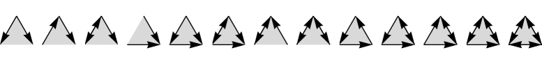
Figure 1: All 13 possible non-isomorphic connected triadic subgraphs (subgraph patterns) in directed unweighted networks.

In order to evaluate the extent of an over- or underrepresentation, for each pattern $i$, the framework commonly used compares its frequency of occurrence in the original network under investigation, $N_{\text{original},i}$, to the expected frequency of occurrence in an ensemble of random networks with the same degree distribution and the same number of unidirectional and bidirectional links as the original network, $\left\langle N_{\text{rand},i}\right\rangle$. Over- and underrepresentation of pattern $i$ is then quantified through a $Z$ score

$$Z_{i}=\frac{N_{\text{original},i}-\left\langle N_{\text{rand},i}\right\rangle}{\sigma_{\text{rand},i}}$$ (1)

where $\sigma_{\text{rand},i}$ represents the standard deviation of $N_{\text{rand},i}$ in the ensemble of the null model. Hence, every network can be assigned a vector $\vec{Z}$ whose components comprise the $Z$ scores of all possible triad patterns of Fig. 1.

However, this approach does not account for potentially existing heterogeneities in graph structures. Suppose, e.g., the feed-forward loop (FFL), , is overrepresented in a certain area of a graph, but, at the same time, highly underrepresented in another part of the graph. On the global network level, the effects may cancel out such that the $Z$ score will be close to zero and possibly relevant structural information will be lost. Therefore, we recently suggested the methodology of Node-Specific Pattern Mining (NoSPaM) [9, 11]. Instead of mining frequent subgraphs on the system level, NoSPaM investigates the neighborhood of every single node separately. I.e., for every node $\alpha$, NoSPaM considers only those triads in which $\alpha$ participates in. Since the position of node $\alpha$ in the triadic subgraphs matters now, the symmetry of most patterns shown in Fig. 1 is broken and the number of connected node-specific triad patterns increases from 13 to 30. These are shown in Fig. 2. To understand the increase in the number of patterns, consider the ordinary subgraph . From the perspective of one particular node, it splits into the three node-specific triad patterns 14, 16, and 23 in Fig. 2. Furthermore, some patterns are included in others, e.g. pattern 1 is a subset of pattern 3. In order to avoid biased results, it is not double counted, i.e. an observation of pattern 3 will only increase its corresponding count and not the one associated with pattern 1 [9, 11].

For every node $\alpha$ in a graph, NoSPaM will compute $Z$ scores for each of the 30 node-specific patterns $i$ shown in Fig. 2,

$$Z_{i}^{\alpha}=\frac{N_{\text{original},i}^{\alpha}-\left\langle N_{\text{rand},i}^{\alpha}\right\rangle}{\sigma_{\text{rand},i}^{\alpha}}.$$ (2)

$N_{\text{original},i}^{\alpha}$ is the number of appearances of pattern $i$ in the triads node $\alpha$ participates in. Accordingly, $\left\langle N_{\text{rand},i}^{\alpha}\right\rangle$ is the expected frequency of pattern $i$ in the triads node $\alpha$ is part of in the ensemble of graphs with the same degree distribution and the same number of both unidirectional and bidirectional links. $\sigma_{\text{rand},i}^{\alpha}$ is the corresponding standard deviation.

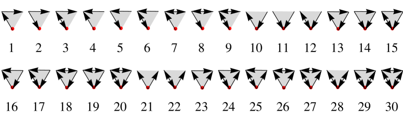
Figure 2: All possible connected, nonisomorphic triadic subgraph patterns in terms of a distinct node (here: lower node).

The following section of this manual provides for information on how to download and run an implementation of NoSPaM. In Section 3, details of the applied algorithms are discussed.

2 How to use NoSPaM

2.1 Download and Installation

• Requirements: make sure to have a recent Java version installed (version 1.7 or higher)

• Download: NoSPaM can be downloaded from www.mwinkler.eu following the Supplementary Material link.

• Extract the

  ospam.zip ~file to whereever you prefer to store \textsc{NoSPaM}.
  \item Go to the comma

  d line terminal and navigate to the nospam directory.

• Generate executable class files by typing: javac *.java

• ^∗In case of problems with the compilation process make sure that the PATH variable includes the JDK, e.g. ’C:\Program Files\Java\jdk1.7.0_11\bin’

• Start a test run by typing: java nospam exampleNetwork.txt 2000 1500

2.2 Running NoSPaM

Input data must be stored in the followig format:

Ψ<source node 1><tab><target node 1>
Ψ<source node 2><tab><target node 2>
Ψ...
Ψ<source node M><tab><target node M>

Every line represents an edge of the network. The identities of the node must be represented by integer values. Any additional entries in a line (e.g. an edge weight) will be ignored by the algorithm. The file type is arbitrary and can be, e.g., .txt, .dat, .csv, etc…

The general command line syntax is as follows:

Ψjava nospam <filePath> <samples> <switching attempts>

• if the network file to be analyzed is already in the nospam directory (e.g. the file exampleNetwork.txt), the variable <filePath> can simply be set to the value <fileName>.<fileType>

• the variable <samples> specifies the number of instances from the randomized ensemble to be used for estimating the average values, $\left\langle N_{\text{rand},i}^{\alpha}\right\rangle$, and the standard deviations, $\sigma_{\text{rand},i}^{\alpha}$.

• the variable <switching attempts> specifies the number of microscopic rewiring steps. It should be chosen proportionally to the number of edges, $|E|$, in the graph and not smaller than $|E|$ (see Section 3 and References [5] and [9] for details).

2.3 Output File

The output of NoSPaM is written in a separate file of the same type as the input file. Fig. 3 gives an example of such an output file. After the header lines, the evaluated data is stored. For each node (indicated by the ids in the first column), the values of $N_{\text{original},i}^{\alpha}$, $\left\langle N_{\text{rand},i}^{\alpha}\right\rangle$, $\sigma_{\text{rand},i}^{\alpha}$, and $Z_{i}^{\alpha}$ are stored in the columns corresponding to the patterns $i$ in Fig. 2.

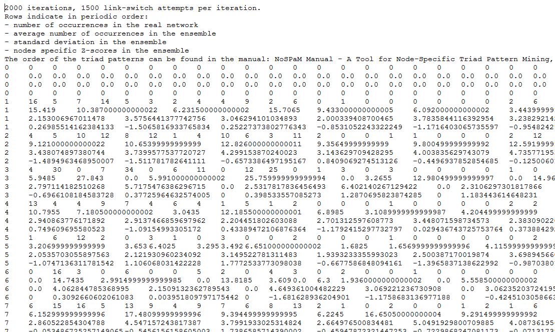
Figure 3: Example output file. The first column indicates the ids of the nodes. The following 30 columns correspond to the node-specific patterns shown in Fig. 2 (in the same order). For every node, there are four lines: the first one indicates the total number of occurrences in the original network, $N_{\text{original},i}^{\alpha}$; the second line indicates the mean number of occurrences in the randomized ensemble, $\left\langle N_{\text{rand},i}^{\alpha}\right\rangle$; the third line indicates the standard deviation in the randomized ensemble, $\sigma_{\text{rand},i}^{\alpha}$; the fourth line indicates the node-specific $Z$ scores which can be obtained from the other three measures.

For the output file shown in Fig. 3, e.g., from the perspective of the node with id 1, pattern 1 () has appeared 16 times in the network under investigation. In the randomized ensemble it appeared 15.42 times on average with a standard deviation of $2.15$ resulting in a $Z$ score, $Z_{i=1}^{\alpha=1}$ of $0.27$ indicating a non-significant overrepresentation of the pattern. Further, pattern 2 () has appeard 5 times in the neighborhood of node 1, while in the randomized ensemble it occurred $10.39$ times on average with a standard deviation of $3.58$ yielding a $Z$ score of $Z_{i=2}^{\alpha=1}=-1.51$ indicating an underrepresentation of the pattern.

3 Algorithms

3.1 Randomization

The generation of the random null model with the same degree distribution and the same number of unidirectional and bidirectional links adjacent to each vertex as in the network under investigation is realized by a link-swapping algorithm. The microscopic switching rules are illustrated in Fig. 4.

The number of microscopic switching attempts is the only parameter of the randomization that needs to be specified in advance. The entire randomization procedure is displayed in Algorithm 1. The Markov chain generated by successive link swappings obeys detailed balance and coverges towards a uniform distribution of the networks in the ensemble serving as the null model, i.e. every valid network is sampled with equal probability. This fact is elaborated in depth in [9]. The number of switching attempts should be chosen proportionally to the number of edges in the graph [5].

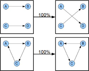
((a))

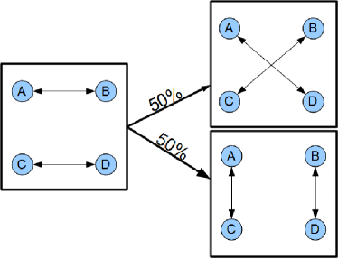
((b))

Figure 4: Microscopic link-switchings performed to generate the randomized ensembles. (a) Pair switch and loop switch for unidirectional links. (b) Pair switch for bidirectional links.

Algorithm 1 Degree-preserving randomization of a graph

function Randomize(Graph $\mathcal{G}\left(V,E\right)$, no. of required steps)

     s = 0

     while s $<$ number of required rewiring steps do

         pick a random link $e_{1}\in E$

         if $e_{1}$ is unidirectional then

              pick a 2nd unidirectional link $e_{2}\in E$ at random

         else

              pick a 2nd bidirectional link $e_{2}\in E$ at random

         end if

         

         if $e_{1}$ and $e_{2}$ do not share a node then

              rewire according to the pair-switch rules in Fig. 4

              if one of the new links already exists then

                  undo the rewiring

              end if

         else if $e_{1}$ and $e_{2}$ participate in a loop then

              rewire according to the loop-switch rule in Fig.4(a)

         end if

         

         s++

     end while

     return randomized instance of $\mathcal{G}$

end function

3.2 Counting of Node-Specific Triad Patterns

For counting the frequencies in which the distinct node-specific triad patterns occur, an iteration over all connected triads is necessary. The procedure is illustrated in Algorithm 2. Because it is computationally expensive to test all triads in the system (the complexity is of order $\mathcal{O}\left(N^{3}\right)$), we rather iterate over pairs of adjacent edges in the graph. Since real-world networks are usually sparse, this is much more efficient [9].

Algorithm 2 Counting of node-specific triad patterns

function NspPatternCounter(Graph $\mathcal{G}(V,E)$)

     $\mathcal{N}$: $N\times 30$-dimensional array storing the pattern counts for every node of $\mathcal{G}$

     for every edge $e\in E$ do

         $i,j$ $\leftarrow$ IDs of $e$’s nodes with $i<j$

         $\mathcal{C}\leftarrow\left\{\right\}$ be list of candidate nodes to form triad patterns comprising $e$

         $\mathcal{C}\leftarrow$ all neighbors of $i$

         $\mathcal{C}\leftarrow$ all neighbors of $j$

         for all $c\in\mathcal{C}$ do

              if $i+j<$ sum of IDs of all other connected

          dyads in triad $(ijc)$ then

                  increase the counts in $\mathcal{N}$ for $i$, $j$, and $c$ for

                  their respective node-specific patterns

              end if

         end for

     end for

     return $\mathcal{N}$

end function

3.3 Node-Specific Triad Pattern Mining

The evaluation of the node-specific $Z$ scores is performed by Algorithm 3. For a more detailed discussion of the algorithms including considerations of the compuational effort see References [11, 9].

Algorithm 3 Node-specific triad pattern mining (NoSPaM)

function NoSPaM(Graph $\mathcal{G}$, # required rewiring steps, # randomized instances)

     $\mathcal{N}_{\text{original}}\leftarrow$ NspPatternCounter($\mathcal{G}$)

     $\mathcal{N}_{\text{rand}}\leftarrow\left\{\right\}$

     $\mathcal{N}_{\text{sq,rand}}\leftarrow\left\{\right\}$

     for # randomized instances do

         $\mathcal{G}\leftarrow$ Randomize($\mathcal{G}$, # required rewiring steps)

         counts $\leftarrow$ NspPatternCounter($\mathcal{G}$)

         $\mathcal{N}_{\text{rand}}\leftarrow\mathcal{N}_{\text{rand}}+$ counts

         $\mathcal{N}_{\text{sq,rand}}\leftarrow\mathcal{N}_{\text{sq,rand}}+$ counts $*$ counts

     end for

     $\mathcal{N}_{\text{rand}}\leftarrow\mathcal{N}_{\text{rand}}/(\#\text{randomized instances})$

     $\mathcal{N}_{\text{sq,rand}}\leftarrow\mathcal{N}_{\text{sq,rand}}/(\#\text{randomized instances})$

     $\mathcal{\sigma}_{\text{rand}}\leftarrow\sqrt{\mathcal{N}_{\text{sq,rand}}-(\mathcal{N}_{\text{rand}}*\mathcal{N}_{\text{rand}})}$

     $\mathcal{Z}\leftarrow(\mathcal{N}_{\text{original}}-\mathcal{N}_{\text{rand}})/\mathcal{\sigma}_{\text{rand}}$

     return $\mathcal{Z}$

end function

References

- [1] I. Albert and R. Albert. Conserved network motifs allow protein-protein interaction prediction. Bioinformatics (Oxford, England), 20(18):3346–52, Dec. 2004.
- [2] U. Alon. Network motifs: theory and experimental approaches. Nature reviews. Genetics, 8(6):450–61, June 2007.
- [3] M. Berlingerio, F. Bonchi, B. Bringmann, and A. Gionis. Mining graph evolution rules. In Machine learning and knowledge discovery in databases, pages 115–130. Springer, 2009.
- [4] R. Milo, S. Itzkovitz, N. Kashtan, R. Levitt, S. Shen-Orr, I. Ayzenshtat, M. Sheffer, and U. Alon. Superfamilies of evolved and designed networks. Science, 303(5663):1538–42, Mar. 2004.
- [5] R. Milo, N. Kashtan, S. Itzkovitz, M. Newman, and U. Alon. On the uniform generation of random graphs with prescribed degree sequences. arXiv preprint cond-mat/0312028, 2004.
- [6] R. Milo, S. Shen-Orr, S. Itzkovitz, N. Kashtan, D. Chklovskii, and U. Alon. Network motifs: simple building blocks of complex networks. Science, 298(5594):824–7, Oct. 2002.
- [7] M. Rahman, M. Bhuiyan, and M. Hasan. Graft: An efficient graphlet counting method for large graph analysis. 2014.
- [8] O. Sporns and R. Kötter. Motifs in Brain Networks. PLoS Biology, 2(11):e369, 2004.
- [9] M. Winkler. On the Role of Triadic Substructures in Complex Networks. epubli GmbH, Berlin, 2015.
- [10] M. Winkler and J. Reichardt. Motifs in triadic random graphs based on Steiner triple systems. Phys. Rev. E, 88(2):022805, Aug. 2013.
- [11] M. Winkler and J. Reichardt. Node-specific triad pattern mining for complex-network analysis. In IEEE International Conference on Data Mining Workshop (ICDMW), pages 605–612, Dec 2014.