A Mixed Basis Density Functional Approach for One-Dimensional Systems with B-splines

Abstract

A mixed basis approach based on density functional theory is extended to one-dimensional (1D) systems. The basis functions here are taken to be the localized B-splines for the two finite non-periodic dimensions and the plane waves for the third periodic direction. This approach will significantly reduce the number of the basis and therefore is computationally efficient for the diagonalization of the Kohn-Sham Hamiltonian. For 1D systems, B-spline polynomials are particularly useful and efficient in two-dimensional spatial integrations involved in the calculations because of their absolute localization. Moreover, B-splines are not associated with atomic positions when the geometry structure is optimized, making the geometry optimization easy to implement. With such a basis set we can directly calculate the total energy of the isolated system instead of using the conventional supercell model with artificial vacuum regions among the replicas along the two non-periodic directions. The spurious Coulomb interaction between the charged defect and its repeated images by the supercell approach for charged systems can also be avoided. A rigorous formalism for the long-range Coulomb potential of both neutral and charged 1D systems under the mixed basis scheme will be derived. To test the present method, we apply it to study the infinite carbon-dimmer chain, graphene nanoribbon, carbon nanotube and positively-charged carbon-dimmer chain. The resulting electronic structures are presented and discussed in details.
PACS: 71.15.Mb, 73.20.-r

I INTRODUCTION

There has been increasing interest in one-dimensional (1D) systems on the nanoscale, such as tubes, wires, rods, ribbons, etc, because the electronic properties of these systems are fundamentally different from those in higher dimensions due to their unusual collective excitations. Expectations concerning the creation and application of improved functional electrodevices with better performance characteristics are rising from the intensive exploration of 1D systems. Particularly, the emergence of nanotechnology has led to the realization of 1D materials and stimulated both academic research and material innovation.

First-principles methods based on the density functional theory have proven to be powerful and successful in investigating the electronic structures and properties of solids. The use of a plane-wave basis is most natural for infinite 3-dimensional periodic systems, such as bulk solids, because of its easy implementation and the fact that the convergence of the calculation can be checked systematically.

To retain all the advantages of plane-wave expansions and of periodic boundary conditions in the investigation of low-dimensional systems, which are finite along the non-periodic direction(s), the conventional supercell approximation is adopted by introducing some artificial vacuum space to separate the periodic replica along the non-periodic direction. However, this approach suffers from one main drawback. For example, in two-dimensional (2D) systems, it requires a vacuum layer of large thickness such that the interactions between the adjacent slabs are negligible, and therefore increases the number of the plane waves along that direction. In particular, for charged systems (e.g. charged defects), the rather long-range tail of the Coulomb potential inevitably requires an extremely large separation of the two slabs and makes the calculation impractical LCC . Many correction schemes have been devised to remedy this difficulty TB -RVMGR . These drawbacks become even more significant in 1D systems.

In previous work LC -RHC , a mixed planar basis approach that is conceptually simple, has successfully been introduced for the first-principles calculations of 2D systems by expanding the wavefunction along the periodic directions with 2D plane waves but, for the finite non-periodic direction, with 1D localized basis of Gaussian functions or B-splines deBoor . The use of this mixed basis has several advantages over the supercell modeling: (1) It resumes the layer-like local geometry which appears in surfaces and describes the wavefunction in a natural way. (2) Because one can calculate the total energy for an isolated slab instead of using a supercell consisting of alternating slab and vacuum regions, the physical quantity, such as the work function can be immediately obtained without any correction. (3) For charged systems, the spurious Coulomb interaction between the defect, its images and the compensating background charge in the supercell approach can be automatically avoided. (4) The number of the basis is significantly reduced, easing the computational burden for the diagonalization of the Kohn-Sham Hamiltonian.

To preserve the above good properties, in the present work, we extend our earlier work RHC to 1D systems, i.e., with two sets of B-splines to expand the wavefunctions along the two finite non-periodic directions and 1D plane waves along the periodic one. B-splines are highly localized and piecewise polynomials within prescribed break points which consist of a sequence numbers called knot sequence deBoor and have proven to be an excellent tool for the description of wavefunctions RHC -RJH . B-splines have the following properties: (1) due to their absolute localization, the relevant matrices are sparse. This is particularly useful and efficient for 1D systems, which involve multi-dimensional spatial integrations. (2) B-splines possess good flexibility to represent a rapidly varying wavefunction accurately with the knots being arbitrarily chosen to have an optimized basis. (3) B-splines are, unlike the atom-centered Gaussian basis, independent of atomic positions, so the geometry optimization can be easily implemented. Here, a rigorous formalism designed to treat the long-range Coulomb potential of both neutral and charged 1D systems within the present mixed-basis framework is also developed.

We apply the present approach to study the infinite carbon-dimmer chain, graphene nanoribbon, carbon nanotube, and the case of positively-charged carbon-dimmer chains. We perform the band structure calculation using Vanderbilt’s ultra-soft pseudopotentials (USPP) DV . Extensive comparisons are made to the standard supercell approach with the popular VASP code KJ ; KF . It is found that the calculated band structures are very promising but the number of the basis is significantly reduced. Aside from the reduction, no further corrections are needed for the charged chain.

II METHOD OF CALCULATION

II.1 B-splines

For the sake of completeness, we first briefly summarize the B-spline formalism. More details can be found in Refs. RHC and deBoor .

B-spline of order $\kappa$ consists of positive polynomials of degree $\kappa-1$, over $\kappa$ adjacent intervals. These polynomials are determined by a knot sequence $\{\tau_{i}\}$ and vanish everywhere outside the subintervals $\tau_{i}<s<\tau_{i+\kappa}$. The B-spline basis set is generated by the following relation :

$$B_{i,\kappa}(s)=\frac{s-\tau_{i}}{\tau_{i+\kappa-1}-\tau_{i}}B_{i,\kappa-1}(s)+\frac{\tau_{i+\kappa}-s}{\tau_{i+\kappa}-\tau_{i+1}}B_{i+1,\kappa-1}(s),$$ (1)

with

$$B_{i,1}(s)=\left\{\begin{array}[]{ll}1,&\tau_{i}\leq s<\tau_{i+1}\\ 0,&{\rm otherwise\ .}\end{array}\right.$$ (2)

The first derivative of the B-spline is given by

$$\frac{d}{ds}B_{i,\kappa}(s)=\frac{\kappa-1}{\tau_{i+\kappa-1}-\tau_{i}}B_{i,\kappa-1}(s)-\frac{\kappa-1}{\tau_{i+\kappa}-\tau_{i+1}}B_{i+1,\kappa-1}(s).$$ (3)

Therefore, the derivative of B-splines of order $\kappa$ is simply a linear combination of B-splines of order $\kappa-1$, which is also a simple polynomial and is continuous across the knot sequence. Obviously, B-splines are flexible to accurately represent any localized function of $s$ with a modest number of the basis by only increasing the density of the knot sequence where it varies rapidly RHC .

II.2 Relevant matrix elements within B-spline basis

In Vanderbilt’s USPP scheme DV , the wavefunction $\phi_{i}$ satisfies a secular equation of the form

$$H|\phi_{i}>=\epsilon_{i}S|\phi_{i}>$$ (4)

under a generalized orthonormality condition

$$<\phi_{i}|S|\phi_{j}>=\delta_{ij}\ .$$ (5)

Here,

$$H=-\nabla^{2}\ +V_{pp}+V_{H}+V_{xc}\ ,$$ (6)

with $V_{pp}$, $V_{H}$, and $V_{xc}$ denoted as the pseudopotential, Hartree potential, and exchange-correlation potential, respectively, and $S$ is a Hermitian overlap operator. In the following, we will give a detailed description of the relevant calculations for $H$ and $S$ operators.

By using two sets of B-splines to describe the non-periodic $x$ and $y$ directions and 1D plane waves for the periodic $z$ direction, the present mixed basis used to expand $\phi_{i}$ is defined as

$$<{\bf r}|{\bf\ k+G};j,\kappa;j^{{}^{\prime}},\kappa^{{}^{\prime}}>\ =\frac{1}{\sqrt{L}}\ e^{i(k+G)z}\ B_{j,\kappa}(x)B_{j^{{}^{\prime}},\kappa^{{}^{\prime}}}(y)$$ (7)

where ${\bf G}$ and ${\bf k}$ denote respectively the reciprocal lattice vector, and the Bloch wave vector. $L$ is the length of the system along the $z$ direction.

We define

$$<\ B_{i,\kappa}|\ B_{i^{\prime},\kappa}>_{s}\ =\int ds\ B_{i,\kappa}(s)\ B_{i^{\prime},\kappa}(s)$$ (8)

where $s=x$ or $y$. It is an integration of local polynomials with bounded support and vanishes unless the condition $|i-i^{\prime}|\leq\kappa$ is fulfilled . This property is particularly useful for higher-dimensional integrals involved in the calculations for 1D systems.

The overlap matrix elements between two basis states are given by

$$<{\bf k+G};i,\kappa;i^{{}^{\prime}},\kappa^{{}^{\prime}}\ |\ {\bf k+G^{\prime}};j,\kappa;j^{{}^{\prime}},\kappa^{{}^{\prime}}>\ =\ <\ B_{i,\kappa}|\ B_{j,\kappa}>_{x}\ <\ B_{i^{\prime},\kappa^{\prime}}|\ B_{j^{\prime},\kappa^{\prime}}>_{y}\ \delta_{G,G^{\prime}}\ .$$ (9)

The kinetic energy matrix elements are given by

$$<{\bf k+G};i,\kappa;i^{{}^{\prime}},\kappa^{{}^{\prime}}\ |\ -\nabla^{2}\ |\ {\bf k+G^{\prime}};j,\kappa;j^{{}^{\prime}},\kappa^{{}^{\prime}}>\$$ (10)

$$= [\ <\ {B^{\prime}}_{i,\kappa}|\ {B^{\prime}}_{j,\kappa}>_{x}\ <\ {B}_{i^{\prime},\kappa^{\prime}}|\ {B}_{j^{\prime},\kappa^{\prime}}>_{y}\ +<\ {B}_{i,\kappa}|\ {B}_{j,\kappa}>_{x}\ <\ {B^{\prime}}_{i^{\prime},\kappa^{\prime}}|\ {B^{\prime}}_{j^{\prime},\kappa^{\prime}}>_{y}\$$ (11)

$$+ <\ {B}_{i,\kappa}|\ {B}_{j,\kappa}>_{x}\ <\ {B}_{i^{\prime},\kappa^{\prime}}|\ {B}_{j^{\prime},\kappa^{\prime}}>_{y}\ (k+G)^{2}\ ]\ \delta_{G,G^{\prime}}\ .$$ (12)

${B^{\prime}}_{i,\kappa}(s)$ is the derivative of $B_{i,\kappa}(s)$. As mentioned above, because of the absolute localization of $B_{i,\kappa}$ and $B^{\prime}_{i,\kappa}$, the evaluation for the kinetic part of $H|\phi_{i}>$ is only an order

$$N_{d}(\kappa-1)\kappa\ ,$$ (13)

where $N_{d}$ is the number of the basis. In practical applications, $\kappa$ is usually set to be 4 or 5. Therefore, the computational effort for the construction of the kinetic energy matrix elements scales linearly as $N_{d}$.

The local part of $V_{pp}$ on each atomic site with species $\sigma$ concerned here was fitted as

$$V_{\text{loc}}^{\sigma}({\bf r})=\ -\ \frac{Z^{\sigma}}{r}\ \text{erf}\left(\frac{r}{R_{c}^{\sigma}}\right)+\sum_{i}A_{i}^{\sigma}e^{-a_{i}^{\sigma}r^{2}}.$$ (14)

Presently, the $d$-like pseudopotential is chosen as the local pseudopotential. The first term on the right hand side of Eq. (14) will be referred to as the core term due to the core charge distribution

$$n_{c}(r)\ =\frac{Z^{\sigma}}{\pi^{\frac{3}{2}}{R_{c}^{\sigma}}^{3}}\ e^{-\frac{r^{2}}{{R_{c}^{\sigma}}^{2}}}\ .$$

The local pseudopotential of the crystal is then given by

$$V_{\text{LOC}}({\bf r})=\sum_{{\sigma,\bf R^{\sigma}}}V_{\text{loc}}^{\sigma}({\bf r}-{\bf R^{\sigma}})\ ,$$ (15)

where ${\bf R^{\sigma}}$ denotes the position of each atom with species $\sigma$. The Fourier transform of the local pseudopotential of the crystal excluding the core term, $V^{\prime}_{\text{LOC}}$, is given by

$$V^{\prime}_{\text{LOC}}(\boldsymbol{\rho},g)\ =\frac{1}{L}\int dz\ V^{\prime}_{\text{LOC}}({\bf r})\ e^{-igz}$$ (16)

$$=\sum_{\sigma,{\bf R_{\parallel}^{\sigma}}\in\ UC}\sum_{i}\left(\frac{A_{i}^{\sigma}}{L_{u}}\right)\sqrt{\frac{\pi}{a_{i}^{\sigma}}}e^{-\ \frac{g^{2}}{4a_{i}^{\sigma}}}\ e^{-a_{i}^{\sigma}(\boldsymbol{\rho-R}_{\parallel}^{\sigma})^{2}}\ .$$ (17)

Here, $L_{u}$ is the length of the unit cell (UC) along $z$ axis.

The total charge distribution $n$ is defined as the sum of the core charge distributions for all atoms in the sample $n_{c}$, plus the electronic charge distributions $n_{e}$,

$$n({\bf r})=n_{c}({\bf r})+n_{e}({\bf r}).$$ (18)

The Coulomb potential $V^{(C)}$ due to the total electron charge distribution and the exchange-correlation potential $V_{xc}$ should be determined self-consistently. The exchange-correlation potential are deduced from the Monte Carlo results calculated by Ceperley and AlderCA and parametrized by Perdew and ZungerPZ . We write

$$V_{xc}({\bf r})=\sum_{g}V_{xc}(\boldsymbol{\rho},g)\ e^{igz}\ .$$ (19)

With the use of the 1D Fourier transformation of $1/r$ (see the Appendix)

$$\frac{1}{r}=\frac{1}{\pi}\int dq_{z}K_{0}(|q_{z}|\rho)\ e^{iq_{z}z}\$$

where $K_{0}$ is the modified cylindrical Bessel function of zero order, the Coulomb potential due to the total charge distribution is given by

$$V^{(C)}=\iiint d^{3}{\bf r^{\prime}}\frac{n({\bf r^{\prime}})}{|{\bf r}-{\bf r^{\prime}}|}$$

$$=\sum_{g}V^{(C)}(\boldsymbol{\rho},g)\ e^{igz}$$ (20)

where

$$V^{(C)}(\boldsymbol{\rho},g)=2\iint d^{2}\boldsymbol{\rho^{\prime}}n({\boldsymbol{\rho^{\prime}}},g)K_{0}(|g||{\boldsymbol{\rho}}-{\boldsymbol{\rho^{\prime}}}|),$$ (21)

with

$$n({\boldsymbol{\rho}},g)=\frac{1}{L}\ \int dz\ n({\bf r})\ e^{-igz}\ .$$

$K_{0}$ will diverge when $g\rightarrow 0$. But, $V^{(C)}(\boldsymbol{\rho},0)$ is still well defined, as explained below.

For the $g\rightarrow 0$ case, using the asymptotic behavior of $K_{0}$

$$K_{0}(x)\rightarrow-\ln x+\ln 2-\gamma,\ \ \ x\rightarrow 0^{+}$$

where $\gamma$ is the Euler-Mascheroni constant, $V^{(C)}(\boldsymbol{\rho},0)$ is now split into two terms,

$$V^{(C)}(\boldsymbol{\rho},0)=2\ (\ln 2-\gamma-\ln|g|)\iint d^{2}\boldsymbol{\rho^{\prime}}n({\boldsymbol{\rho^{\prime}}},0)-2\iint d^{2}\boldsymbol{\rho^{\prime}}n({\boldsymbol{\rho^{\prime}}},0)\ln(|{\boldsymbol{\rho}}-{\boldsymbol{\rho^{\prime}}}|)\ .$$ (22)

The first term could be safely dropped if the system is charge neutral ($\iint d^{2}\boldsymbol{\rho^{\prime}}n({\boldsymbol{\rho^{\prime}}},0)=0$). We demonstrate in the following that omitting such term still holds for charged systems.

We assume $L$, the length of the system along the $z$ direction, is arbitrarily large but finite. With

$$n({\bf r})=\sum_{g}\ n({\boldsymbol{\rho}},g)\ e^{igz}\ ,$$ (23)

the $g=0$ component of $V^{(C)}$ will be

$$V^{(C)}(\boldsymbol{\rho},0)=\iiint_{-L/2}^{L/2}\frac{dz^{\prime}}{\sqrt{\Delta\boldsymbol{\rho}^{2}+z^{\prime 2}}}\ n({\boldsymbol{\rho^{\prime}}},0)\ d^{2}\boldsymbol{\rho^{\prime}}$$ (24)

where $\Delta\boldsymbol{\rho}=|{\boldsymbol{\rho}}-{\boldsymbol{\rho^{\prime}}}|$. Suppose $L$ be much larger than the cell size in the $xy$ plane, i.e., $L\gg\Delta\boldsymbol{\rho}$, then

$$\int_{0}^{L/2}\frac{dz^{\prime}}{\sqrt{\Delta\boldsymbol{\rho}^{2}+z^{\prime 2}}}=\ln\frac{L/2+\sqrt{L^{2}/4+\Delta\boldsymbol{\rho}^{2}}}{\Delta\boldsymbol{\rho}}\sim\ln L-\ln|\Delta\boldsymbol{\rho}|\ .$$ (25)

So,

$$V^{(C)}(\boldsymbol{\rho},0)=2\ln L\iint d^{2}\boldsymbol{\rho^{\prime}}\ n({\boldsymbol{\rho^{\prime}}},0)-2\iint d^{2}\boldsymbol{\rho^{\prime}}\ n({\boldsymbol{\rho^{\prime}}},0)\ln|{\boldsymbol{\rho}}-{\boldsymbol{\rho^{\prime}}}|.$$ (26)

In the case of charge neutrality, the first term on the right hand side of Eq. (26) vanishes and we retain Eq. (22). For charged systems with net line charge density $N_{l}=\iint d^{2}\boldsymbol{\rho^{\prime}}\ n({\boldsymbol{\rho^{\prime}}},0)\neq 0$, such term would be huge. But clearly it is a constant that is independent upon $\boldsymbol{\rho}$, and only causes a shift to the total energy. This kind of constant is irrelevant to the band structure calculation. Therefore, within the present mixed basis approach, we could, just like the charge-neutral case, omit the first term without further corrections for the charged systems.

The numerical integration around the singularity at ${\boldsymbol{\rho}}={\boldsymbol{\rho^{\prime}}}$ in Eqs. (21) and ( 22) can be carried out and averaged over one finer sub-grid unit. In practice, we perform such an integration over a circle $C$, whose area is equal to that of the grid unit, as shown in Fig. 1. We also assume $n(\boldsymbol{\rho^{\prime}})$ be constant within such a circle. Then,

$$2\iint_{C}d^{2}\boldsymbol{\rho^{\prime}}n({\boldsymbol{\rho^{\prime}}},g)K_{0}(|g||{\boldsymbol{\rho}}-{\boldsymbol{\rho^{\prime}}}|)\ \sim\ 4\pi n(\boldsymbol{\rho},g)\left[\frac{1}{g^{2}}-\frac{\epsilon}{|g|}K_{1}(\epsilon|g|)\right],$$ (27)

and

$$-2\iint_{C}d^{2}\boldsymbol{\rho^{\prime}}n({\boldsymbol{\rho^{\prime}}},0)\ln(|{\boldsymbol{\rho}}-{\boldsymbol{\rho^{\prime}}}|)\sim\ -n(\boldsymbol{\rho},0)\left[\epsilon^{2}\ln\epsilon-\frac{1}{2}\epsilon^{2}\right].$$ (28)

Here, $\epsilon$ is the radius of the circle $C$ and $K_{1}$ is the modified Bessel function of order 1.

We define the total local potential $V_{\text{eff}}$ as

$$V_{\text{eff}}=V^{(C)}+V_{xc}+V^{\prime}_{\text{LOC}}\ .$$ (29)

To construct the $V_{\text{eff}}|\phi_{i}>$, we need to calculate $<{\bf k+G};i,\kappa;i^{{}^{\prime}},\kappa^{{}^{\prime}}\ |V_{\text{eff}}|\phi_{i}>$ in the real-space. Again, it can be done efficiently with the advantage of the absolute localization of B-splines mentioned before.

Now, lets turn to the nonlocal part of $H$. The atomic nonlocal potential in the Kleinman-Bylander (KB) form KB is given as

$$V_{\text{nl}}^{\sigma}({\bf r}-{\bf R^{\sigma}})=\sum_{nlmn^{\prime}l^{\prime}m^{\prime}}D_{nlm,n^{\prime}l^{\prime}m^{\prime}}^{\sigma,{\bf R^{\sigma}}}|\beta_{n,lm}^{\sigma,{\bf R^{\sigma}}}><\beta_{n^{\prime},l^{\prime}m^{\prime}}^{\sigma,{\bf R^{\sigma}}}|\ ,$$ (30)

with

$$D_{nlm,n^{\prime}l^{\prime}m^{\prime}}^{\sigma,{\bf R^{\sigma}}}=D_{nl,n^{\prime}l^{\prime}}^{0,\sigma}\delta_{l,l^{\prime}}\delta_{m,m^{\prime}}+\iiint d^{3}{\bf r}V_{\text{eff}}({\bf r})Q_{nlm,n^{\prime}l^{\prime}m^{\prime}}^{\sigma}({\bf r}-{\bf R^{\sigma}})\ .$$ (31)

The projector $\beta_{n,lm}^{\sigma}$ and the augmentation function $Q_{nlm,n^{\prime}l^{\prime}m^{\prime}}^{\sigma}$ vanish outside the atomic core region. $\beta_{n,lm}^{\sigma,{\bf R^{\sigma}}}$ denotes the projector centered at the ${\bf R^{\sigma}}$ atom, i.e., $\beta_{n,lm}^{\sigma,{\bf R^{\sigma}}}=\beta_{n,lm}^{\sigma}({\bf r}-{\bf R^{\sigma}})$.

The nonlocal pseudopotential of the crystal is

$$V_{\text{NL}}({\bf r})=\sum_{\sigma,{\bf R^{\sigma}}}V_{\text{nl}}^{\sigma}({\bf r}-{\bf R^{\sigma}})\ .$$ (32)

In practical calculations, we define a box, which is large enough to contain the core region LPCLV . The $\beta_{n,lm}^{\sigma}(\boldsymbol{\rho-R}_{\parallel}^{\sigma},z)$ inside the box is transferred to ${\bf G}$ space, then

$$\beta_{n,lm}^{\sigma,{\bf R^{\sigma}}}=\beta_{n,lm}^{\sigma}({\bf r}-{\bf R^{\sigma}})=\sum_{G}\beta_{n,lm}^{\sigma}(\boldsymbol{\rho-R}_{\parallel}^{\sigma},G)\ e^{-iGR_{z}^{\sigma}}\ e^{iGz}\ .$$ (33)

Therefore,

$$<{\bf k+G};i,\kappa;i^{{}^{\prime}},\kappa^{{}^{\prime}}\ |\beta_{n,lm}^{\sigma,{\bf R^{\sigma}}}>\\ =\ e^{-i(k+G)R_{z}^{\sigma}}\sum_{G^{{}^{\prime}}}\iint d^{2}\boldsymbol{\rho}\ B_{i,\kappa}(x)B_{i^{\prime},\kappa^{\prime}}(y)\ \beta_{n,lm}^{\sigma}(\boldsymbol{\rho-R}_{\parallel}^{\sigma},G^{\prime})\int dz\ \ e^{i(G^{\prime}-G-k)z}\ .$$ (34)

Similarly, both $Q_{nlm,n^{\prime}l^{\prime}m^{\prime}}^{\sigma}({\bf r}-{\bf R^{\sigma}})$ and $V_{\text{eff}}({\bf r})$ in Eq. (31) are also transferred by fast Fourier transfer (FFT),

$$Q_{nlm,n^{\prime}l^{\prime}m^{\prime}}^{\sigma}({\bf r}-{\bf R^{\sigma}})=\sum_{G_{h}}Q_{nlm,n^{\prime}l^{\prime}m^{\prime}}^{\sigma}(\boldsymbol{\rho-R}_{\parallel}^{\sigma},G_{h};R_{z}^{\sigma})\ e^{iG_{h}z}\ ,$$ (35)

$$V_{\text{eff}}({\bf r})=\sum_{G_{h}}V_{\text{eff}}(\boldsymbol{\rho},G_{h})\ e^{iG_{h}z}\ .$$ (36)

Then, we obtain

$$D_{nlm,n^{\prime}l^{\prime}m^{\prime}}^{\sigma,{\bf R^{\sigma}}}=D_{nl,n^{\prime}l^{\prime}}^{0,\sigma}\delta_{l,l^{\prime}}\delta_{m,m^{\prime}}+L_{b}^{\sigma}\sum_{G_{h}}\iint d^{2}\boldsymbol{\rho}\left[V_{\text{eff}}(\boldsymbol{\rho},G_{h})\right]^{*}Q_{nlm,n^{\prime}l^{\prime}m^{\prime}}^{\sigma}(\boldsymbol{\rho-R}_{\parallel}^{\sigma},G_{h};R_{z}^{\sigma})\ .$$ (37)

$L_{b}^{\sigma}$ is the length of the core region box along the $z$ axis. Note that the FFT grid density for $G_{h}$ in the summation of Eqs. (35) and (36) is not necessarily the same with that for the wavefunction LPCLV . $D_{nlm,n^{\prime}l^{\prime}m^{\prime}}^{\sigma,{\bf R^{\sigma}}}$ in the above should be calculated self-consistently. From Eqs. (34) and (37), we can evaluate $V_{\text{NL}}|\phi_{i}>$. In doing this, we need to calculate

$$<{\bf k+G};j,\kappa;j^{{}^{\prime}},\kappa^{{}^{\prime}}\ |V_{\text{NL}}|\phi_{i}>=\sum_{\sigma,{\bf R^{\sigma}}}\sum_{nlmn^{\prime}l^{\prime}m^{\prime}}D_{nlm,n^{\prime}l^{\prime}m^{\prime}}^{\sigma,{\bf R^{\sigma}}}<{\bf k+G};j,\kappa;j^{{}^{\prime}},\kappa^{{}^{\prime}}\ |\beta_{n,lm}^{\sigma,{\bf R^{\sigma}}}><\beta_{n^{\prime},l^{\prime}m^{\prime}}^{\sigma,{\bf R^{\sigma}}}|\phi_{i}>\ .$$ (38)

Because of the KB separation form in Eq. (38), the computation effort for this part is also linear to $N_{d}$.

As for the Hermitian overlap operator $S$, which is peculiar to the Vanderbilt USPP scheme, it is given by

$$S=I+\sum_{\sigma,{\bf R^{\sigma}}}\sum_{nlmn^{\prime}l^{\prime}m^{\prime}}q_{nlm,n^{\prime}l^{\prime}m^{\prime}}^{\sigma}|\beta_{n,lm}^{\sigma,{\bf R^{\sigma}}}><\beta_{n^{\prime},l^{\prime}m^{\prime}}^{\sigma,{\bf R^{\sigma}}}|\ ,$$ (39)

where $q_{nlm,n^{\prime}l^{\prime}m^{\prime}}^{\sigma}=\iiint d^{3}{\bf r}Q_{nlm,n^{\prime}l^{\prime}m^{\prime}}^{\sigma}({\bf r})$. $S|\phi_{i}>$ will be obtained similarly. Finally, the charge density from the wave function is augmented inside the core region,

$$\rho_{e}({\bf r})=\sum_{i}[\ |\phi_{i}({\bf r})|^{2}+\sum_{\sigma,{\bf R^{\sigma}}}\sum_{nlmn^{\prime}l^{\prime}m^{\prime}}Q_{nlm,n^{\prime}l^{\prime}m^{\prime}}^{\sigma}({\bf r}-{\bf R^{\sigma}})<\phi_{i}|\beta_{n,lm}^{\sigma,{\bf R^{\sigma}}}><\beta_{n^{\prime},l^{\prime}m^{\prime}}^{\sigma,{\bf R^{\sigma}}}|\phi_{i}>\ ].$$ (40)

To find the lowest eigenvectors of the Hamiltonian matrix $H$, we used the Lanczos-Krylov method developed previously RHC , with the orthonormality of the wavefunctions maintained throughout by the standard Gram-Schmidt orthogonalization procedure.

III APPLICATIONS OF PRESENT METHOD

III.1 infinite carbon-dimmer chain

For the first example, we study a simple testing case of infinite carbon-dimmer chains, as shown in the top panel of Fig. 2. The chain has a periodicity of $\sqrt{3}a_{0}$ ($a_{0}=2.461~{}$Å) along the $z$ axis and the atom distance of C-C is chosen to $a_{0}/\sqrt{3}$. Two sets of 11 B-splines that each is defined over a range of 3.25 $a_{0}$, are used to expand the $x$ and $y$-component wavefunction, respectively. The energy cutoff of the 1D plane waves along the $z$ axis is 20 Ry. Special $k$-points of 1/8 and 3/8 (in unit of $2\pi/\sqrt{3}a_{0}$) were taken to sample the 1D Brillouin zone. The C USPP was generated from the Vanderbilt’s code vancode and its quality was examined previously RHC . For comparison, we also performed the calculation by using the VASP code with the projector-augmented-wave potential (PAW) KJ ; KF . A typical vacuum space of 10 Å $\times\ 10$ Å  required in VASP was used in the calculation. The potential is determined self-consistently until its change is less than $10^{-6}$ Ry.

Figure 2(a) displays the band structure between $\Gamma$ (0) and $X$ (1/2). The VASP counterpart is shown in Fig. 2(b). Clearly, the present calculation agrees nicely with that by VASP. The splitting of the twofold degenerate bands due to the symmetry of the system is found to be smaller than 0.0001 eV. Note that the number of the basis is significantly reduced from $\sim 4300$ by VASP to $\sim 1900$ by the present method.

III.2 graphene nanoribbon

Next, in order to provide a stringent test of the present method, a realistic system of the armchair graphene nanoribbon is considered. The width of the ribbon here is chosen to include $N_{a}=19$ carbon dimmer lines, as indicated in the left part of Fig. 3. One set of 73 B-splines distributed over a range of 14.25 $a_{0}$ and another of 11 B-splines over a range of 3.25 $a_{0}$ were used to expand the $x$- and $y$-components of the wavefunction, respectively. The energy cutoff of the 1D plane waves for the periodic direction was 20 Ry. The atomic positions of the system were taken from Ref. RHC . The special $k$-points for sampling the 1D Brillouin zone are 1/8 and 3/8.

The present band structures near the Fermi level are displayed in Fig. 3(a). To make a comparison, we also show the previous calculations and VASP results RHC in Figs. 4(b) and (c), respectively. In previous work RHC , we adopted the planar mixed basis set to study the nanoribbon by using the surface supercell modeling for the $x-z$ plane. Namely, we used only one set of B-splines to expand the $y$ component of the wavefunction. As compared with the VASP calculation, which was obtain by the traditional 3-dimensional supercell modeling, the total number of the basis in previous work RHC is reduced from $\sim$17000 to $\sim$12300. Now, if we use another set of B-splines for the $x$ non-periodic direction, then the number is further reduced to 8800 only. However, it can be seen from the figures that there is a very nice agreement between these three approaches. This reflects the advantage of using B-splines for non-periodic directions over the plane waves, especially for 1D systems. Actually, we have done all the calculations of the $N_{a}<19$ families. All the results are found in excellent agreements with those by VASP. Therefore, we are convinced that the present program has been implemented successfully for 1D systems and the results obtained are very reliable. Moreover, as compared to the traditional supercell modeling, the use of the present mixed basis will significantly reduce the number of the basis functions and speed up the calculations for 1D systems.

III.3 zigzag carbon nanotube

Now, we study carbon nanotubes (CNTs), allotropes of carbon with a cylindrical nanostructure. We choose the (4,0) zigzag CNT (Fig. 4) as the third example.

A mixed basis set with two identical sets of 29 B-splines over a range of 6.25 $a_{0}$ along the two non-periodic directions and the plane wave cutoff of 20 Ry along the periodic direction are used. All C atoms were kept at the ideal positions which were obtained by rolling the ideal graphene sheet with the C-C bond length taken to be $a_{0}/\sqrt{3}$. The special $k$-point for sampling the 1D Brillouin zone was 1/4. The resultant band structures are presented in Fig. 4(a), along with the VASP calculations in Fig. 4(b) for comparison.

Clearly, all bands compare favorably with those by VASP. It is worth mentioning that it would be more efficient to investigate nanotubes or rods if we expand the wavefunction in cylindrical coordinates rather than in Cartesian ones. Here, we utilize this system to test the present program. With the present algorithm to study CNT, the B-splines used are more densely distributed as compared to the first two cases. And the relevant real-space integrations were carried out with finer grids (48 equal divisions within $a_{0}$) to obtain precise results. Nevertheless, the total number of the basis used here is reduced from $\sim$9700 by VASP to $\sim$8000 by the present mixed-basis approach. To sum up, we have demonstrated that the present program is computationally efficient to produced reliable results.

III.4 charged carbon-dimmer chain

Finally, we apply the present method to charged systems which are very challenging for the supercell modeling because of the spurious long-range Coulomb interaction between the defect and its periodic images. For simplicity, we still use the same system of the infinite carbon-dimmer chain, but here with one of every eight electrons removed. That is, the nominal ionicity of C in this artificial positively-charged chain is +0.5. All other computational conditions are similar to the first example described above. The resulting band structure is shown in Fig. 5(a). We also show the VASP result in Fig. 5(b), which was obtained by using a homogeneous compensating background charge.

It is obvious that the present approach yields very similar results to those by VASP. Notably, the convergence rate of the calculation is fast and comparable to the neutral case. In the supercell approach, the charged defects are unfortunately subjected to the spurious image interaction, and no supercell size in practice would be sufficient to render this long-ranged electrostatic interaction negligible. Various types of corrections have been proposed to remove the interactions between the charged defect, its image, and the background charge TB -RVMGR . On the other hand, in the mixed-basis approach, it is natural to drop the logarithmically divergent term of Eq. (26) that has similar effect to the cancellation between the electrostatic energies from the defects and the uniform compensating background assumed in the supercell model. No further corrections are needed in our scheme since only one single isolated charged system rather than an array of the replicated ones is under consideration. Hence, we have developed an alternative promising method to study both neutral and charged 1D systems with no complications.

IV CONCLUSIONS

In conclusion, we have successfully extended the previous mixed-basis approach to investigate the electronic structures of one-dimensional systems with plane waves for the periodic direction and B-spline sets for the two non-periodic directions. As compared to the existing algorithms based upon the conventional supercell model with alternating slab and vacuum regions, it is a real space approach along the two non-periodic directions. Therefore, the number of the basis functions used to expand the wavefunction is significantly reduced and the spurious Coulomb interaction between the defect, its images and the compensating background charge appeared in the supercell approach can be automatically avoided.

The new technique has been demonstrated to yield accurate and computationally efficient treatments of the infinite carbon-dimmer chain, graphene nanoribbon, carbon nanotube, and the system of the positively-charged chain. It is found that the band structures are all in good agreement with those by the popular existing codes, but with a reduced number of basis functions. Moreover, no further corrections are needed for the charged case. We have shown that the present method is very suitable to investigate either neutral or charged 1D materials without the need of artificially large supercells or corrections for supercell interactions.

*

Appendix A

$$\frac{1}{r} = \frac{4\pi}{(2\pi)^{3}}\iiint\frac{e^{i{\bf q}{\bf r}}}{q^{2}}d^{3}{\bf q}$$ (41)

$$= \frac{1}{2\pi^{2}}\iiint\frac{e^{i{\boldsymbol{q}_{\parallel}}{\boldsymbol{\rho}}}}{q_{\parallel}^{2}+q_{z}^{2}}d^{2}{\boldsymbol{q}_{\parallel}}\ {e^{i{q_{z}}{z}}}dq_{z}$$ (42)

$$= \frac{1}{2\pi^{2}}\iiint\frac{e^{i{q_{\parallel}}{\rho}\cos\phi}}{q_{\parallel}^{2}+q_{z}^{2}}q_{\parallel}dq_{\parallel}d\phi\ {e^{i{q_{z}}{z}}}dq_{z}\ .$$ (43)

With the identity

$$J_{0}(x)=\frac{1}{2\pi}\int_{0}^{2\pi}e^{ix\cos\phi}d\phi$$ (44)

where $J_{0}$ is the Bessel function of order 0,

$$\frac{1}{r}=\frac{1}{\pi}\iint\frac{{J_{0}(q_{\parallel}{\rho})}}{q_{\parallel}^{2}+q_{z}^{2}}q_{\parallel}dq_{\parallel}\ {e^{i{q_{z}}{z}}}dq_{z}\ .$$ (45)

Using another identity

$$\int_{0}^{\infty}\frac{xJ_{0}(ax)}{x^{2}+k^{2}}dx=K_{0}(ak)\ \ \ [a>0,{\rm Re}\ k>0]$$ (46)

We obtain

$$\frac{1}{r}=\frac{1}{\pi}\int dq_{z}K_{0}(|q_{z}|\rho)\ e^{iq_{z}z}\ .$$ (47)

Fig. 1: Schematic plot of the grid unit containing the singularity at ${\boldsymbol{\rho}}={\boldsymbol{\rho^{\prime}}}$ for the Coulomb potential. See text for details.

Fig. 2: (Color online) (top) Atomic structure of the infinite carbon-dimmer chain. (a) and (b) are the corresponding band structures obtained by the present work and VASP.

Fig. 3: (Color online) (left) Atomic structure of the armchair graphene nanoribbon. (a), (b) and (c) are the band structures near Fermi level by the present work, previous work RHC and VASP, respectively.

Fig. 4: (Color online) (top) Atomic structure of the (4,0) zigzag carbon nanotube. (a) and (b) are the band structures obtained by the present work and VASP.

Fig. 5: (Color online) The band structures of the positively charged carbon-dimmer chain obtained by (a) the present work and (b) VASP with a uniform background charge.

Figure 1:

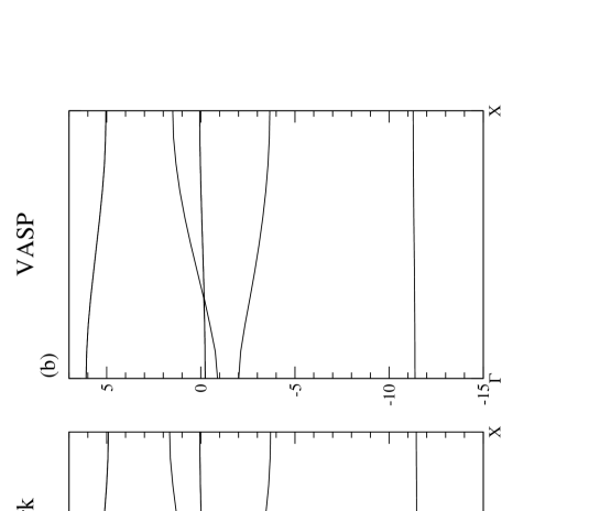
Figure 2:

Figure 3:

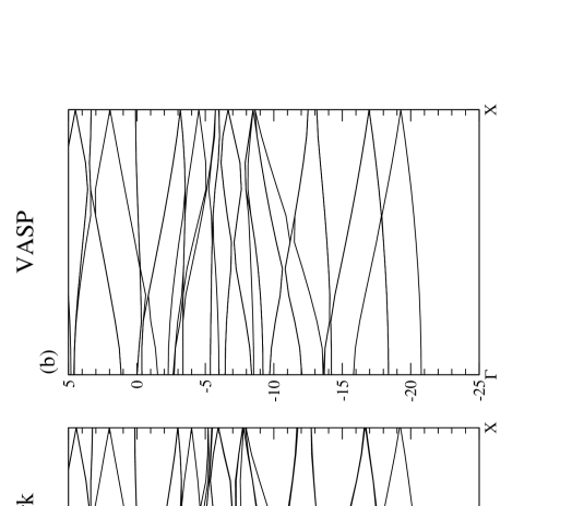
Figure 4:

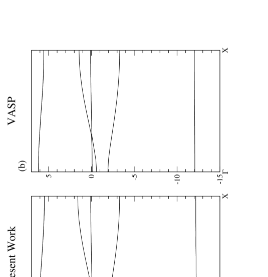
Figure 5:

References

- (1) A. J. Lee, T.-L. Chan, and J. R. Chelikowsky, Phys. Rev. B 89, 075419 (2014).
- (2) S. E. Taylor and F. Bruneval, Phys. Rev. B 84, 075155 (2011), and references therein.
- (3) G. Makov and M. C. Payne, Phys. Rev. B 51, 4014 (1995).
- (4) C. A. Rozzi, D. Varsano, A. Marini, E. K. U. Gross, and A. Rubio, Phys. Rev. B 73, 205119 (2006).
- (5) G.-W. Li and Y.-C. Chang, Phys. Rev. B 48, 12032 (1993).
- (6) G.-W. Li and Y.-C. Chang, Phys. Rev. B 50, 8675 (1994).
- (7) Y.-C. Chang and G.-W. Li, Comp. Phys. Comm. 95, 158 (1996).
- (8) C. Y. Ren, C. S. Hsue and Y.-C. Chang, Comp. Phys. Comm. 188, 94 (2015).
- (9) Carl deBoor, A practical Guide to Splines, (Springer, New York, 1987).
- (10) W. R. Johnson, S. A. Blundell, and J. Sapirstein, Phys. Rev. A 37, 307 (1988).
- (11) H. T. Jeng, and C. S. Hsue, Phys. Rev. B 62, 9876 (2000).
- (12) C. Y. Ren, H. T. Jeng, and C. S. Hsue, Phys. Rev. B 66, 125105 (2002).
- (13) D. Vanderbilt, Phys. Rev. B 41, 7982 (1990).
- (14) G. Kresse and D. Joubert, Phys. Rev. B 59, 1758 (1999).
- (15) G. Kresse and J. Furthmüller, Comput. Mater. Sci. 6, 15 (1996).
- (16) D. M. Ceperley and B. J. Alder, Phys. Rev. Lett. 45, 566 (1980).
- (17) J. P. Perdew and A. Zunger, Phys. Rev. B 23, 5048 (1981).
- (18) L. Kleinman and D. M. Bylander, Phys. Rev. Lett. 48, 1425 (1982).
- (19) K. Laasonen, A. Pasquarello, R. Car, C. Lee, and D. Vanderbilt, Phys. Rev. B 47, 10142 (1993).
- (20) http://www.physics.rutgers.edu/ dhv/uspp/.
FIGURE CAPTIONS