Simulated Navier-Stokes trefoil reconnection

Abstract

The evolution and self-reconnection of a perturbed trefoil vortex knot is simulated, then compared to recent experimental measurements (Scheeler et al., 2014a). Qualitative comparisons using three-dimensional vorticity isosurfaces and lines, then quantitative comparisons using the helicity. To have a single initial reconnection, as in the experiments, the trefoil is perturbed by 4 weak vortex rings. Initially there is a long period with deformations similar to the experiment during which the energy, continuum helicity and topological self-linking number are all preserved. In the next period, once reconnection has clearly begun, a Reynolds number independent fraction of the initial helicity is dissipated in a finite time. In contrast, the experimental analysis finds that the helicity inferred from the trajectories of hydrogen bubbles is preserved during reconnection. Since vortices reconnect gradually in a classical fluid, it is suggested that the essential difference is in the interpretation of the reconnection timescales associated with the observed events. Both the time when reconnection begins, and when it ends. Supporting evidence for the strong numerical helicity depletion is provided by spectra, a profile and visualisations of the helicity that show the formation of negative helicity on the periphery of the trefoil. A single case with the same trajectory and circulation, but a thinner core, replicates this helicity depletion despite larger Sobolev norms, showing that the reconnection timescale is determined by the initial trajectory and circulation of the trefoil, not the initial vorticity. This case also shows that the very small viscosity, $\nu\rightarrow 0$ mathematical restrictions upon finite-time dissipative behavior do not apply to this range of modest viscosities.

1 Background

An intrinsic property of a field of twisted and linked vortices is its helicity ${\cal H}$, the volume integral of the helicity density $h=\mbox{\boldmath$u$}\cdot\mbox{\boldmath$\omega$}$ (4). This integral is conserved by the inviscid equations and in a turbulent flow the helicity density can move through scales in a manner similar to the cascade of kinetic energy (2), the other quadratic inviscid invariant. However, a well-defined role for helicity in turbulent dynamics remains elusive (Moffatt, 2014). Reasons for this include the difficulties in imposing physical space helical structures, in both experiments and simulations, as well as identifying analysis tools distinct from those used to study the energy cascade that can define what helical structures and dynamics are.

Kleckner & Irvine (2013) have recently demonstrated one way to investigate helicity experimentally. This is to imprint helical vortex structures into a classical fluid by yanking 3D-printed aerofoil knots, covered with hydrogen bubbles out of a water tank. The vortices shed by the aerofoil are then visualised by the hydrogen bubbles which are shed along with the vortices and align themselves into filaments along the low pressure vortex cores. Once the trajectories of these filaments are known, then estimates of the helicity can be determined from the topology of the filaments. This can be done by determining the linking, twist and writhe of the filaments, then multiplying each of these by their circulations to estimate the helicity (13), without knowing either the velocity and vorticity.

The purpose of this paper is to simulate the most complicated configuration of Kleckner & Irvine (2013), a trefoil vortex, using the initial condition shown in figure 1. Then address the following. First, make qualitative comparisons with the experimental trefoil visualisations in Scheeler et al. (2014a, b) to demonstrate the relevance of these simulations to their experiment. Next, address their surprising claim that the trefoil preserves its helicity during reconnection. Third, discuss how the unique characteristics of the trefoil make it an ideal tool for investigating the regularity of the Navier-Stokes equation in ways that other initial configurations cannot.

Generating a trefoil vortex is challenging, both experimentally and numerically. The challenge is to weave, but not link, a vortex of finite diameter and fixed circulation into a (3,2) knot. That is, a knot with three crossings over two loops whose self-linking number (10) is ${\cal L}_{S}={\cal W+T}=3$. In a classical fluid, the resulting global helicity is exactly ${\cal H}=\Gamma^{2}{\cal L}_{S}$, where $\Gamma$ is the circulation of the vortex (Laing et al., 2015). The additional challenge for these simulations is to have only one initial reconnection, as in the experiments. Instead of the three simultaneous reconnections that an ideal trefoil generates (Kida & Takaoka, 1987).

The characteristics of the trefoil that make it ideal for investigating the regularity properties of the Navier-Stokes and Euler equations are the following: First, unlike other configurations such as initially anti-parallel or orthogonal vortices, it has finite energy in an infinite domain. Second, it should self-reconnect due to how the two loops cross three times when the trefoil is projected into its direction of propagation. Third, opposing this tendency, because the initial helicity is nearly maximal, it can be used to investigate how helicity suppresses nonlinearities. Fourth, it can be simulated in a periodic box, making detailed Fourier analysis using Sobolev norms possible.

The surprising result from the trefoil vortex knot experiment was that their measure of the helicity was preserved over the entire reconnection. Unlike their linked ring case, whose helicity noticeably decayed as the reconnection generated a gap between the vortices. The diagrams, but not necessarily the underlying bubble patterns, in Kleckner & Irvine (2013) and Scheeler et al. (2014a) suggest that there has also been complete reconnection to the simpler knots for the trefoil, even though its helicity has not changed.

Do the simulations agree, or disagree, with these experimental result? The answer appears to be a bit of both, if one considers the possibility that the first reconnection event of the experimental trefoil has been misinterpreted. In the new simulations, the trefoil’s helicity is also preserved longer than the helicity for previous configurations using vortices with similar radii and circulations (Kerr, 2005a, 2013a) . However, once reconnection does start, in the simulations there is finite helicity dissipation in a finite time as the viscosity goes to zero. This might be the true significance to the trefoil. It allows us to see the finite-time, finite-dissipation of a macroscopic property: The helicity.

This paper is organised as follows. First, the equations and diagnostics used will be given. Then, the initialisation of the vortex is described, with the result illustrated in figure 1. The similarities between the early evolution generated by this initial condition and the early evolution of the experimental trefoil, that is until reconnection begins for both, is demonstrated using the isosurfaces and vortex lines in figures 2 ($t=24$) and 5 ($t=31$). The remaining three-dimensional figures are then introduced, followed by the quantitative diagnostics that can tell us when reconnection begins (traditional vorticity norms in figure 4) and when helicity decays (helicity and its partner norms in figure 4). These timescales underlie the comparisons that follow between the dissipation isosurfaces given in figure 6 and the experimental movie that can be accessed through Scheeler et al. (2014b). Spectra, a profile and helicity isosurfaces are then used to interpret the origins of the helicity dissipation in terms of a dual cascade, that is a cascade with oppositely signed helicity componets moving to opposite scales in both physical space and Fourier space. At the end is a discussion how the observed finite-helicity depletion might be influenced by the current mathematical constraints upon the regularity of the Navier-Stokes equation.

1.1 Equations and continuum diagnostics

The governing equations for the simulations in this paper will be the incompressible ($\nabla\cdot{\mbox{\boldmath$u$}}=0$) Navier-Stokes equations in a periodic box and the numerical method will be a pseudo-spectral code with a very high wavenumber cut-off filter (Kerr, 2013a).

$$\frac{\partial\mbox{\boldmath$u$}}{\partial t}-\underbrace{\nu\triangle{\mbox{\boldmath$u$}}}_{\rm dissipation}+({\mbox{\boldmath$u$}}\cdot\nabla){\mbox{\boldmath$u$}}=-\nabla p\,.$$ (1)

The equations for its energy, enstrophy and helicity densities, $e=\mbox{$\frac{1}{2}$}\mbox{\boldmath$u$}^{2}$, $\mbox{\boldmath$\omega$}^{2}$ and $h=\mbox{\boldmath$u$}\cdot\mbox{\boldmath$\omega$}$ respectively, and their volume-integrated norms are:

$$\frac{\partial e}{\partial t}+({\mbox{\boldmath$u$}}\cdot\nabla)e=-\nabla p-\underbrace{\nu\triangle{\mbox{\boldmath$u$}}}_{\epsilon={\rm dissipation}},\quad E=\mbox{$\frac{1}{2}$}\int\mbox{\boldmath$u$}^{2}dV\,.$$ (2)

$$\frac{\partial\mbox{\boldmath$\omega$}^{2}}{\partial t}+({\mbox{\boldmath$u$}}\cdot\nabla)\mbox{\boldmath$\omega$}^{2}=\underbrace{\mbox{\boldmath$\omega$}\mbox{\boldmath$S$}\mbox{\boldmath$\omega$}}_{Z_{p}-{\rm production}}+\underbrace{\nu(\nabla\mbox{\boldmath$\omega$})^{2}}_{\epsilon_{\omega}={\rm dissipation}},\quad Z=\int\mbox{\boldmath$\omega$}^{2}dV\,.$$ (3)

$$\frac{\partial h}{\partial t}+({\mbox{\boldmath$u$}}\cdot\nabla)h=\underbrace{-\mbox{\boldmath$\omega$}\cdot\nabla\Pi}_{\omega-{\rm transport}}+\underbrace{\nu\mbox{\boldmath$\triangle$}h}_{\nu-{\rm transport}}-\underbrace{2\nu{\rm tr}(\nabla\mbox{\boldmath$\omega$}\cdot\nabla\mbox{\boldmath$u$}^{T})}_{\epsilon_{h}={\rm dissipation}}\qquad{\cal H}=\int\mbox{\boldmath$u$}\cdot\mbox{\boldmath$\omega$}dV\,,$$ (4)

where $\mbox{\boldmath$\omega$}=\nabla\times\mbox{\boldmath$u$}$ is the vorticity vector and $\Pi=p-\mbox{$\frac{1}{2}$}\mbox{\boldmath$u$}^{2}$. The two quadratic, inviscid ($\nu=0$) invariants are the energy $E$ and helicity ${\cal H}$ (Moffatt, 1969). Unlike the energy, helicity can be of either sign, is not Galilean invariant and can grow due to its viscous terms (Biferale & Kerr, 1995). The enstrophy $Z$ can also grow due to its production term $Z_{p}$.

One can also determine spectra, the spectral transfer of energy and a variety of higher-order Lebesgue $\|u\|_{L^{p}}$ and Sobolev $\|u\|_{\dot{H}^{s}}$ norms:

$$\|u\|_{L^{p}}=\left(\frac{1}{V}\int dV|\mbox{\boldmath$u$}|^{p}\right)^{1/p}\quad{\rm and}\quad\|u\|_{\dot{H}^{s}}=\left(\int d^{3}k|\mbox{\boldmath$k$}|^{2s}|\mbox{\boldmath$u$}(\mbox{\boldmath$k$})|^{2}\right)^{1/2}\,.$$ (5)

The vorticity diagnostics in this paper will be:

$$\omega_{p}=\sup|\mbox{\boldmath$\omega$}|=\|\mbox{\boldmath$\omega$}\|_{\infty}=\|\mbox{\boldmath$\omega$}\|_{L^{\infty}}\quad{\rm and}\quad Z=\|\mbox{\boldmath$\omega$}\|_{2}^{2}=\left(\|u\|_{\dot{H}^{1}}\right)^{2}\,,$$ (6)

plus the normalised enstrophy production, or velocity-derivative skewness,

$$-S_{u}=C_{S}\frac{Z_{p}}{Z}^{3/2}$$ (7)

where $C_{S}$ is a constant relating this isotropic property to the original anisotropic hot-wire measurements of the velocity derivative skewness ($S_{u}$).

The following two diagnostics, with the same dimensional scaling as the helicity, will be shown in figure 4:

$$L^{3}=\|u\|_{L^{3}}\quad{\rm and}\quad H^{(1/2)}=\|u\|_{\dot{H}^{1/2}}\,.$$ (8)

Control of these norms has been shown to be critical to our understanding of the regularity of the Navier-Stokes equations (Escauriaza et al., 2003; Seregin, 2011).

1.2 Vortex lines and linking numbers

To provide comparisions to the experimental vortex lines, figures 1, 5 and 6 include vortex lines ${\cal C}_{i}$ defined by trajectories $\mbox{\boldmath$x$}_{j}(s)$ determined by the Matlab streamline algorithm applied to the vorticity vector field. This algorithm solves the following ordinary differential equation:

$$\frac{d\mbox{\boldmath$x$}_{j}(s)}{ds}=\mbox{\boldmath$\omega$}(\mbox{\boldmath$x$}_{j}(s))$$ (9)

starting from seed positions $\mbox{\boldmath$x$}_{j}(0)$. These seeds were chosen from the positions around, but not necessarily at, local vorticity maxima.

The four topological numbers introduced by Moffatt & Ricca (1992) for generating helicity are: The intervortex linking numbers ${\cal L}_{ij}$ between distinct vortex trajectories ${\cal C}_{i}$ and ${\cal C}_{j}$. The writhe ${\cal W}_{i}$ and twist ${\cal T}_{i}$ numbers of a given vortex. And their sum, the self-linking number:

$${\cal L}_{Si}={\cal W}_{i}+{\cal T}_{i}\,.$$ (10)

The ${\cal L}_{ij}$ and ${\cal L}_{Si}$ for closed loops will be integers (Pohl, 1968), but that is not a requirement for either the writhe ${\cal W}$ or the twist ${\cal T}$.

The quantitative tool that will be used to determine the writhe, self-linking and intervortex linking will be a regularised Gauss linking integral.

$${\cal L}_{ij}=\sum_{ij}\frac{1}{4\pi}\oint_{{\cal C}_{i}}\oint_{{\cal C}_{j}}\frac{(d\mbox{\boldmath$x$}_{i}\times d\mbox{\boldmath$x$}_{j})\cdot\mbox{\boldmath$x$}_{i}-\mbox{\boldmath$x$}_{j}}{(|\mbox{\boldmath$x$}_{i}-\mbox{\boldmath$x$}_{j}|^{2}+\delta^{2})^{1.5}}\,,$$ (11)

where $\delta=0$ when $i\neq j$ and for the calculating the self-linking ${\cal L}_{S}$, which can be obtained by choosing two parallel trajectories of the type illustrated in figure 1. These trajectories can be thought of as the edges of a vortex ribbon. The writhe ${\cal W}_{i}$ is defined by taking $i=j$ in (11) (Calugareanu, 1959) and requires a small, but finite, $\delta$ to get consistent results from this numerical data. The twist ${\cal T}_{i}$ can be determined from the line integral of the Frenet-Serret torsion of the vortex lines:

$${\cal T}_{i}=\frac{1}{2\pi}\oint\tau ds,\qquad{\rm where}\quad\tau=\frac{d\mbox{\boldmath$N$}}{ds}\cdot\mbox{\boldmath$B$}\,.$$ (12)

$N$ and $B$ are the normal and bi-normal Frenet-Serret unit vectors along the trajectories. The focus in this paper will be on the self-linking ${\cal L}_{Si}$, the most robust of these numbers. ${\cal L}_{Si}$ will also provide a useful diagnostic during the later stages of reconnection when it became impossible to find trajectories that formed closed loops.

Obtaining reliable values for the ${\cal L}_{S}$, ${\cal W}$ and ${\cal T}$ numbers was not straightforward using this numerical data due to the irregularities in the trajectories of the vortices determined using (9). Smoothing the resulting trajectories would help, but the following procedures were used instead.

• For ${\cal L}_{S}$, using two independently determined trajectories starting from near, but not identical, seed points was better than adding a push given by either the curvature $N$ or bi-normal $B$ vectors to the original trajectory due to noise in the variations of $N$ and $B$ along the trajectory.

• Obtaining consistent writhe ${\cal W}$ numbers required using very small, but still finite, $\delta$ in (11).

• The difficulty in calculating the twist is that three derivatives of $\mbox{\boldmath$x$}_{j}(s)$ are needed to calculate the torsion $\tau$. Reducing twist to a sum helps: ${\cal T}_{i}=(2\pi)^{-1}\underset{s}{\Sigma}~{}d\mbox{\boldmath$N$}(s)\cdot\mbox{\boldmath$B$}(s)$. However, values from neighbouring trajectories still varied by about 20%. Therefore, all the twist numbers in this paper will be the difference between the self-linking ${\cal L}_{S}$ and the writhe ${\cal W}$.

Once the linking, writhe and twist numbers have been determined, if the vortices have distinct cores, each with a well-defined circulations $\Gamma_{i}$, then the helicity of the flow is exactly (Laing et al., 2015)

$${\cal H}=2\sum_{ij}\Gamma_{i}\Gamma_{j}{\cal L}_{ij}+\Gamma_{i}^{2}{\cal L}_{Si}\,.$$ (13)

The factor of 2 on the ${\cal L}_{ij}$ terms is needed because a link has two crossings in planar projections, instead of the single crossings one gets for a writhe or twist.

While these trajectories are useful in identifying the initial topological changes due to reconnection, they are not used here for $t>31$ because they very rarely formed closed loops. Therefore, the continuum helicity (4) will be the primary diagnostic for identifying changes in the topology during reconnection. Helicity can be applied even when the location and local alignment of the reconnecting vortices are difficult to identify.

Helicity, instead of vorticity norms, will also be used to address regularity properties. The trefoil’s vorticity norms (6) are used to identify important timescales, but are not used for regularity questions because their growth is only modest. So modest that the energy dissipation $\epsilon=\nu Z\rightarrow 0$ as $\nu\rightarrow 0$.

2 Physical space initialisation

The goal of the physical space initialisation is to map an analytically defined trefoil vortex onto an Eulerian (static) numerical mesh. The trefoil trajectories discussed in this paper are defined by:

$$\begin{array}[]{rl}x(\phi)=&r(\phi)\cos(\alpha)\\ y(\phi)=&r(\phi)\sin(\alpha)\\ z(\phi)=&0.5\cos(\alpha)\\ {\rm where}\quad r(\phi)=&r_{t}+r_{1}a\cos(\phi)+a\sin(w\phi+\phi_{0})\\ {\rm and}\quad\alpha=&\phi+a\cos(w\phi+\phi_{0})/(wr_{t})\end{array}$$ (14)

with $r_{t}=2$, $a=0.5$, $w=1.5$, $\phi_{0}=0$, $r_{1}=0.25$ and $\phi=[1:4\pi]$. This weave winds itself about the following perturbed ring: $(r(\phi)-2)^{2}+z^{2}=1$ where $r(\phi)=r_{t}+r_{1}a\cos(\phi)$.

If one chooses $r_{1}=0$, one gets the traditional trefoil with a three-fold symmetry. The symmetric trefoil generates three simultaneous reconnection events at the three crossings of the trefoil loops, which is what the Gross-Pitaevski calculation in Scheeler et al. (2014a) and the Navier-Stokes calculation in Kida & Takaoka (1987) find.

The $r_{1}\neq 0$ perturbation was added in the hope that with this minor adjustment, the trefoil would have a single initial reconnection, similar to what the evolution of the experimental, hydrogen-bubble trajectories show (Scheeler et al., 2014a). This was not sufficient to break the three-fold symmetry, as explained below.

Profile and direction Once the trajectory of the trefoil is established, then the surrounding vorticity profile and vorticity direction needs to be mapped onto the computational mesh. The basis for this mapping is described in Kerr (2013a). It starts by identifying the closest locations on each filament at every mesh point and the distances between these filament locations and the mesh points. These are then used to provide that filament’s contribution to the vorticity vector at the mesh points, a vector whose direction is given by the tangent to the filament at the specified location and whose magnitude is given by inserting the filament’s distance into that filament’s vorticity profile. The profile function is based upon the Rosenhead regularisation of a point vortex:

$$|\omega|(r)=\Gamma\frac{r_{0}^{2}}{(r^{2}+r_{0}^{2})^{2}}\,.$$ (15)

In addition, for every mesh point two points on the trefoil are needed. One point from each loop. To avoid overcounting, the space perpendicular to the central $z$ axis is divided into octants. First, the octant containing the mesh point is found. Then the nearest points on the two loops are found from that octant, plus its two neighbouring octants.

After the profile has been mapped only the mesh, the field is then smoothed with a $k^{4}$ hyperviscous filter. This effectively increases the radius of the profile such that for calculations Q05 to Q00625 with $r_{0}=0.25$, the effective radius based upon the initial peak vorticity $\omega_{0}$ is $r_{eff}=(\Gamma/\omega_{0})^{1/2}=0.47$ and for the case R05 with a thinner core, $r_{0}=0.175$, $r_{eff}=0.33$.

The $r_{0}=0.25$ trefoil after a short time is given in figure 1. The isosurface is a distance of $r\approx 0.25$ from the line originating at $\omega_{m}$ in the centre. The three lengths that define this trefoil are: The radius of the trefoil $r_{t}=2$. The separation between the loops within the trefoil $\delta_{x}=2a=1$. And the pre-filtered profile radius of $r_{0}=0.25$.

First calculations For all of the calculations presented in this paper $r_{1}=0.25$, which yields a perturbed trefoil similar to the experimental initial condition. Unfortunately it does not generate a single initial reconnection as in the experiment and instead relaxes into the three-fold symmetry of an ideal trefoil before slowly diffusing into a single wavy vortex ring.

Increasing the perturbation coefficient $r_{1}$ to values as high as 1.5 did not change this scenario, even though the initial perturbed structure looked nothing like the experimental hydrogen-bubble trefoils.

Clearly some other type of perturbation is needed. It was pointed out that the platform that the trefoil model was placed upon probably generated additional independent vortices that would not have been identified by the hydrogen bubbles in the experiment. Therefore, four low intensity vortex rings propagating either in $+z$ or $-z$ were placed on the periphery of the trefoil to give it the type of external perturbation that the platform might have generated.

Final initial condition The result of adding the four rings to the perturbed trefoil is given in figure 1 at $t=6$, shortly after the calculation began. The two diagnostics are a isosurface of 0.55max($\|\omega\|_{\infty}$) and two closed vortex filaments through the centre of the trefoil (9).

Since this initial state is generated in a periodic box, an important question is whether periodic boundaries might influence the trefoil’s evolution and appearance. To test this possibility, case Q05 was run in a $(4\pi)^{3}$ box. This did not change its appearance or any of the primary diagnostics. A related question is whether the energy or other norms increase as the periodic domain is made larger. If the initial condition were a simple vortex ring the energy would increase, but if one takes two colliding rings as in Lu & Doering (2008), the energy has an upper bound as the periodic domain is made larger. Where does the trefoil sit? This is important for the regularity questions discussed in Sec. 4.

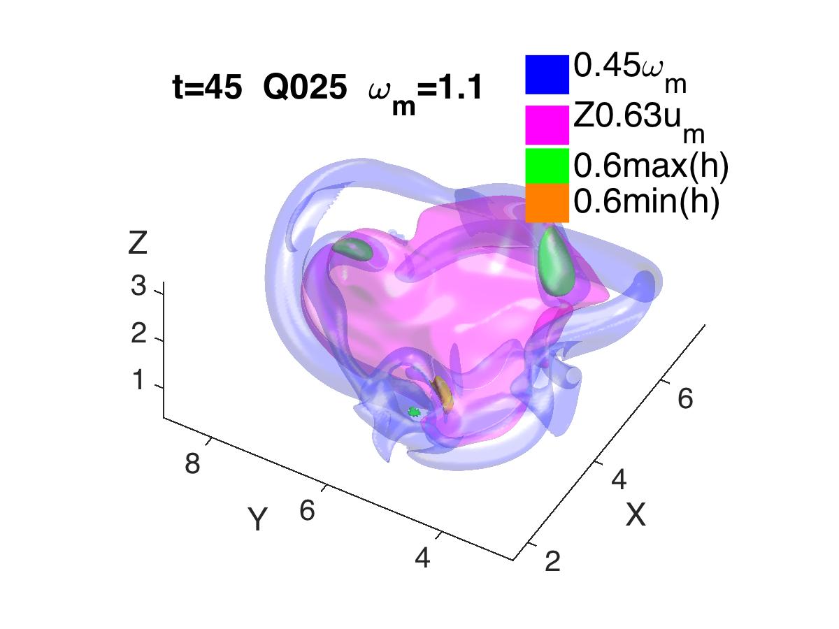
Figure 11: Vorticity, energy and helicity isosurfaces of at $t=45$. Vorticity is indicated by the blue, energy by magenta, large positive helicity by green and large-magnitude negative helicity by orange. The main point is that large values of the energy are entirely confined within the trefoil, without any signs of the type of jets above and below the knot that would be found for a vortex ring.

Figure 10 shows the effects of changing size of the periodic box from $(2\pi)^{3}$ to as large as $(16\pi)^{3}$ upon several norms. Most importantly, the kinetic energy and $L_{3}=\|u\|_{L^{3}}$ do not grow significantly once the box is larger than $(3\pi)^{3}$. The energy profile in figure 8 and the three-dimensional isosurface plot of the energy in figure 11 both show that the energy is almost entirely confined to the interior of the trefoil and does not have the type of jets above and below the knot that would be expected if this were a vortex ring.

Five calculations are discussed. All use the same perturbed trefoil trajectory, a circulation of $\Gamma=0.22$ and the same profile function (but different radii). Plus the same additional weak perturbing vortex rings just mentioned. For the four primary calculations, Q05 to Q00625, the radius of their profile is chosen such that $\omega_{0}=\|\mbox{\boldmath$\omega$}\|_{\infty}(t=0)=1$ For the fifth, the initial core is narrower so that $\|\mbox{\boldmath$\omega$}\|_{\infty}(t=0)=1.9$. The highest Reynolds number simulation, with $\nu=6.25\times 10^{-5}$, has $Re_{\Gamma}=\Gamma/\nu=3500$, Based upon a review of when reconnection begins in several past calculations, (Kerr, 2005b, 2013a) the relevant nonlinear timescale will not be $\omega_{0}^{-1}$, but instead will be

$$t_{x}=2\delta_{x}^{2}/\Gamma=9\,,$$ (16)

where $\delta_{x}=2a=1$ is the separation of the two loops within the trefoil. $t_{x}$ is the same for both of the initial conditions here.

For the trefoil experiment in Scheeler et al. (2014a, b), the initial condition has $r_{t}\approx 50$mm, $a\approx 25$mm and if the initial vortex radius is taken to be the leading edge of the aerofoil, $r_{0}=4$mm. Ratios is closer to case R05 than the cases Q05 to Q00625. The experimental Reynolds number is $Re_{\Gamma}=2\times 10^{4}$, an order of magnitude larger. The equivalent nonlinear timescale based upon putting the experimental values into (16) gives $t_{x}\approx 80$ms, but the figure for Movie S4 in Scheeler et al. (2014b) suggests that $t_{x}\approx 200$ms, so this is used in the comparisons here. Physical space vortex lines, including their topological properties, will be the primary tools for comparisons between the simulations and the experimental diagnostics obtained from the hydrogen bubble visualisations,

Cases	$r_{0}$	$\omega_{\rm in}$	smooth4	$\omega_{0}$	$Z_{0}$	$\nu$	Final Mesh
Q05	0.25	1.26	0.00005	1	$6.5\times 10^{-3}$	$5\times 10^{-4}$	$512^{3}$
Q025	0.25	1.26	0.00005	1	$6.5\times 10^{-3}$	$2.5\times 10^{-4}$	$1024^{3}$
Q0125	0.25	1.26	0.00005	1	$6.5\times 10^{-3}$	$1.25\times 10^{-4}$	$1024^{3}$
Q00625	0.25	1.26	0.00005	1	$6.5\times 10^{-3}$	$6.25\times 10^{-5}$	$2048^{3}$
R05	0.175	2.5	0.0000125	1.9	$1.2\times 10^{-2}$	$5\times 10^{-4}$	$1024^{3}$

Table 1: Parameters for the initial conditions, initial peak vorticity $\omega_{0}=\|\mbox{\boldmath$\omega$}\|_{\infty}(t=0)$, initial enstrophy $Z_{0}$, viscosity of the run and final mesh. The initial helicity for all of the calculations is ${\cal H}(t=0)=7.67\times 10^{-4}$. The initialisation parameters are: The filament’s radius, the pre-filtering input peak vorticity $\omega_{\rm in}$ and the smoothing to: $\exp(-{\rm smooth}\,k^{4})$.

3 Results

The evolution of the trefoil reconnection will be divided into three parts. First, an helicity-invariant period leading up to the beginning of reconnection at $t\approx 30$. Next, a short period with only small changes to the helicity, but clear changes in the topology in the immediate vicinity of the reconnection. Then a longer, final period where these transformations are completed and during which there are significant and finite changes in the helicity.

An overview of the changes to three-dimensional structure during these periods will be illustrated using the following five figures: Figure 1 at $t=6$ to illustrate the initial state. Figure 2 at $t=24$ to illustrate the changes just before reconnection. Figure 5 at $t=31$ to demonstrate how the reconnection begins. Figure 6 at $t=36$, which has the first clear signs of reconnection. And figure 9 at $t=63$ shows the helicity isosurfaces of both signs at the end of reconnection. Figure 11 has been added to highlight how the kinetic energy is localised within the trefoil.

To show how the trefoil core disintegrates over time and to provide a reference for the additional properties in these figures, all six figures include one relatively large value vorticity isosurface. These are supplemented with a variety of additional isosurfaces of vorticity, helicity, dissipation and energy, plus vortex lines.

Figure 6 at $t=36$ has the most additional information. This is to support a proposal, outlined at the end of section 3.4, that the topological changes identified as the first and second reconnection events in the experiments could instead be viewed as two phases of a single reconnection event.

Most of the early time ($t=6,31,36$) three-dimensional graphics are taken from case Q05 with $\nu=5\times 10^{-4}$. Vorticity isosurfaces from case Q025 with $\nu=2.5\times 10^{-4}$ showed only minimal differences in these qualitative large-scale features. Greater differences were evident at later times, so case Q025 is used for the $t=45$ and $t=63$ figures.

After the qualitative overview using these visualisations, more quantitative diagnostics are discussed.

3.1 Overall evolution

Figure 1 at $t=6$ is used to illustrate the initial condition using a single isosurface and two vortex lines obtained using different seeds around the position of maximum vorticity. The self-linking number using (11) is ${\cal L}_{S}=3$.

Figure 2 at $t=24$ provides a planar view with the position of $\omega_{m}=\|\mbox{\boldmath$\omega$}\|_{\infty}$ marked by a red cross along with two added low magnitude helicity isosurfaces. These isosurfaces are for 0.05max($h$) and 0.05min($h$), where $\max(h)=0.22$ and $\min(h)=-0.085$. The structure to the right of $\omega_{m}$ shows that the two loops are beginning to hook around one another to form a locally anti-parallel alignment, foreshadowing the transformation needed for the upcoming reconnection. Also note the $h<0$ yellow regions in the upper left and bottom near the other two loop crossings. These are forming in the directions away from red cross and are a result of the $\omega$-transport term in the helicity equation (4), with $h<0$ moving in one direction and $h>0$ moving in the opposite direction. While still weak because $|\max(h)|>>|\min(h)|$, this transport of helicity along the vortex lines, $h>0$ moving towards the dissipation sites around the reconnection and $h<0$ in the opposite direction, is how negative helicity eventually migrates outside the original trefoil zone, as indicated in figure 9 at $t=63$.

Figure 5 at $t=31$ shows three lines in addition to its single isosurface. The green trajectory originates from near, but not at, X, the point of $\omega_{m}$, and retains the basic trefoil structure, including circumnavigating the central $z$ axis twice. The point between the closest approach of its two loops is indicated by the orange cross, about which these two segments have adopted an anti-parallel orientation, consistent with the argument for why the total linking number might be preserved during anti-parallel reconnections (Laing et al., 2015). Now consider the line between these anti-parallel points and through the orange cross. The red and blue trajectories are seeded from points near the orange cross and in opposite directions perpendicular to this line. Each of these trajectories circumnavigates the central axis only once before returning to its origin, making them rings. Rings that stay within the envelope of the original trefoil and are linked through one another as they pass through the reconnection zone.

On this basis, the orange cross, and not X should be viewed as the reconnection point. The twists of opposing polarity near X on the red and green trajectories are the basis for the comparisons to S4 experimental trefoil movie (Scheeler et al., 2014b) in Sec. 3.3.

Figure 6 at $t=36$ uses a variety of isosurfaces to show the immediate effects of the reconnection. The view has been rotated by about 90^∘ with respect to the view in figure 5 so that the reconnection zone can be seen directly and an evolved version of the green trefoil from figure 5 is included to help orient the viewer. There are two isosurfaces of vorticity, the lower one at $0.11\omega_{m}$ in cyan, to show the envelope of the original trefoil, the second at $0.28\omega_{m}$ in green to emphasise where vorticity remains large. It and the helicity isosurface of $0.15\max(h)$ in blue also show a gap near $[x,y]=[5.5,4.75]$, which is where the reconnection began at $t=31$. The dominant large-scale vorticity structure, indicted by the $0.11\omega_{m}$ isosurface, is still a trefoil.

Added to these are isosurfaces of dissipation and one of helicity advection at $0.5\max\bigl{(}(\mbox{\boldmath$u$}\cdot\nabla)h\bigr{)}$ in purple. The dissipation isosurfaces are for enstrophy dissipation, $0.5\max(\epsilon_{\omega})$ (3), in orange, and for helicity dissipation (4) of both signs, $h=0.5\max(h_{\epsilon})$ in red-brown and $h=0.5\min(h)$ yellow. These are discussed in section 3.3.

Figure 9 at $t=63$ shows a later stage of the reconnection process. To support the evidence from helicity spectra and profiles for the creation of large-scale negative helicity, a planar view is used. The dominant vorticity structure has not been investigated in detail, but vortex lines suggest that what remains of the trefoil has been transformed into a single twisted ring.

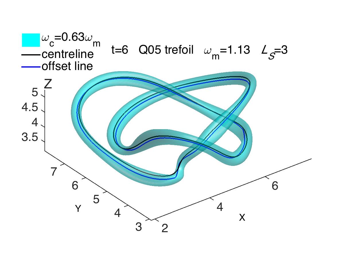
Figure 1: Vorticity isosurface plus two closed vortex lines of the perturbed trefoil vortex at $t=6$, not long after initialization. Its self-linking is ${\cal L}_{S}=3$, which can be split into writhe ${\cal W}=3.15$ and twist ${\cal T}=-0.1$.

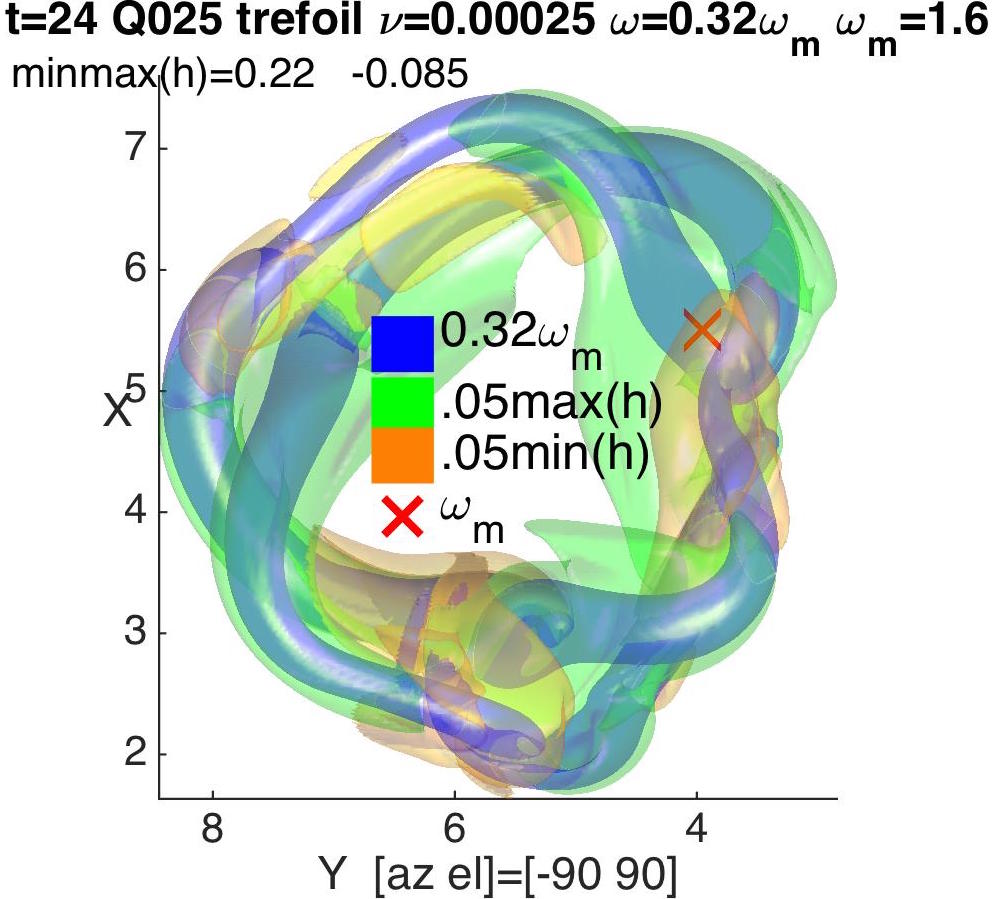
Figure 2: Isosurfaces at $t=24$, shortly before reconnection begins. The vorticity isosurface is in blue and the helicity isosurfaces are of $0.05\max(h)$ in green and $0.05\min(h)$ in yellow where $\max(h)=-0.22$ and $\min(h)=0.085$. The position of $\omega_{m}=\|\mbox{\boldmath$\omega$}\|_{\infty}$, where reconnection is about to begin, is indicted by the red cross.

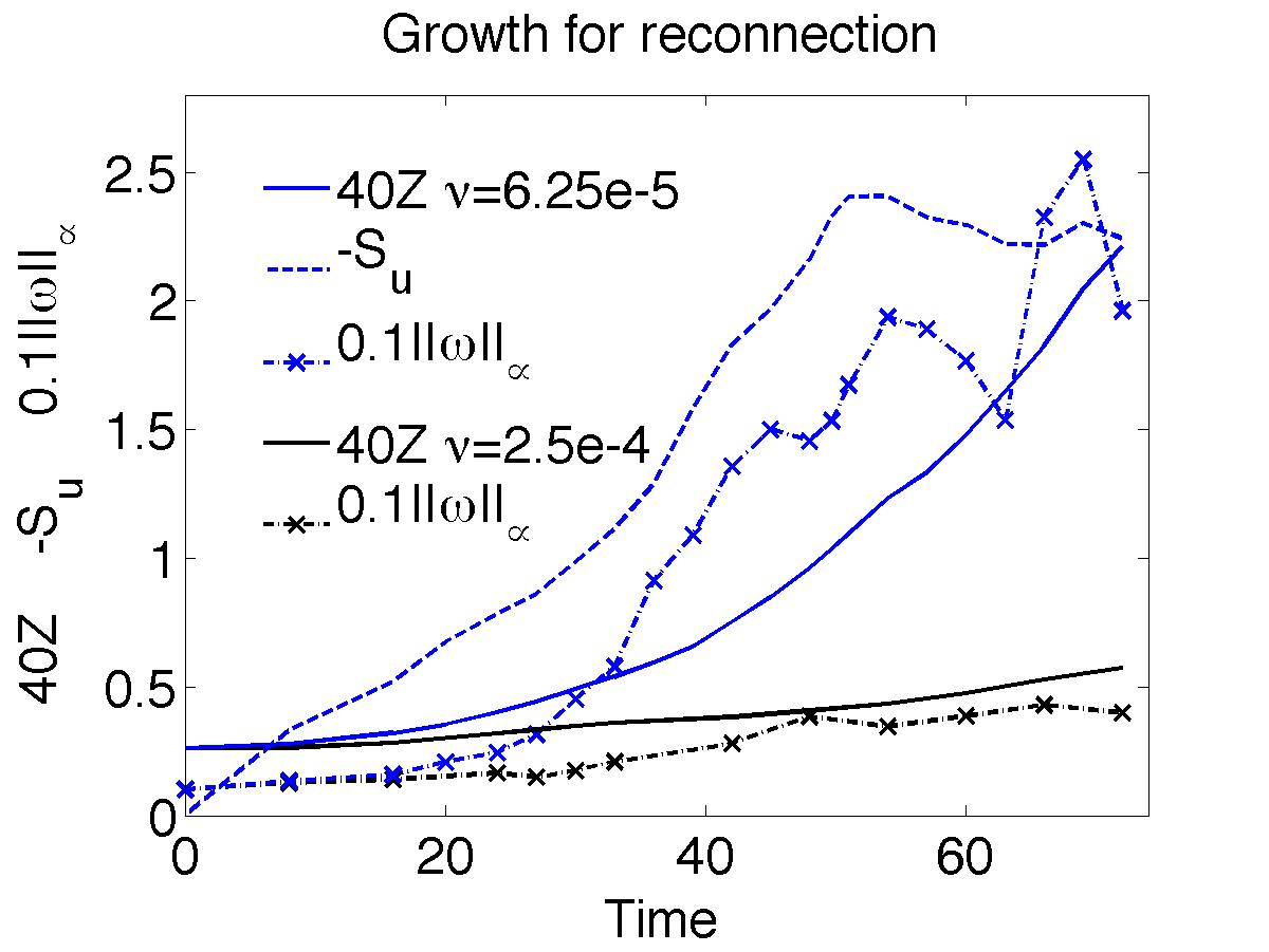
Figure 3: Time evolution of the scaled enstrophy $40Z$, normalized production $S_{u}$ and scaling maximum vorticity $0.1\|\mbox{\boldmath$\omega$}\|_{\infty}$ for two cases. Q025 with $\nu=2.5\times 10^{-4}$ and Q00625 with $\nu=6.25\times 10^{-5}$.

Figure 4: Time evolution of the normalised helicity $({\cal H}L)^{1/2}$ for 4 viscosities: $\nu=0.0005$ to $\nu=0.0000625$. By $t\approx 72$ all 4 cases have roughly the same decrease in helicity. Not shown is case R05 with a thinner core and $\nu=5\times 10^{-4}$, whose helicity decay is almost identical to case Q025 with $\nu=2.5\times 10^{-4}$. Inset shows normalised $L_{3}$ and $H^{(1/2)}=\|u\|_{\dot{H}^{1/2}}$ for two of the calculations. $L_{3}$, $H^{(1/2)}$ and ${\cal H}$ are all normalised to have the units of circulation. $H^{(1/2)}$ must bound both $L_{3}$ and $|{\cal H}|$ from above and increases slowly, as required by its upper bound of $\sqrt{2EZ}$. None of which prevents the strong decrease in ${\cal H}$.

3.2 Quantitative diagnostics

To complement this qualitative picture of the reconnection process, quantitative vorticity and helicity-related diagnostics are provided by figures 4 and 4.

Figure 4 gives three vorticity norms: $\|\mbox{\boldmath$\omega$}\|_{\infty}$ and $Z$ (6), which are scaled, plus the production skewness $-S_{u}$ (7), which is not scaled. $S_{u}$ is not scaled because its unscaled values can tell us the following: It has long been known from both experiments and simulations that $-S_{u}\sim 0.5-0.7$ in fully developed turbulence. What is less appreciated is that for almost all initial conditions since the original pseudo-spectral paper (Orszag & Patterson, 1972), $-S_{u}$ initially overshoots these values. And based upon how strong the overshoot is, $-S_{u}$ can indicate whether finite energy dissipation as the viscosity goes to zero is possible, or whether the dissipation goes to zero as $\nu\rightarrow 0$.

For the trefoil, all of these vorticity norms have significant growth over the period of these calculations, growth that increases as the viscosity decreases. The strong growth starts around $t=30$, setting the timescale for when reconnection begins, and continues for all three norms continues until $t\approx 50$ in all cases. At that time the production skewness saturates at a value of $-S_{u}\approx 2.5$ in the case Q00625, $\nu=0.0000625$. Telling us that for $t>50$, the enstrophy $Z$ cannot grow more than exponentially fast.

While $-S_{u}=2.5$ might seem large, compared to isotropic turbulence values of $-S_{u}\approx 0.7$, the dependence of this saturation value upon the viscosity is weak. So weak that less than 1% of the energy is dissipated in the $\nu=0.0000625$ calculation. That is, for $t_{h}=72$

$$\Delta E_{\nu}=\int_{0}^{t_{h}}dt\,\epsilon=\int_{0}^{t_{h}}dt\,\nu Z~{}<~{}1\%E(t=0)\,.$$

While these vorticity norms have only modest growth, the helicity in figure 4 tells a different story. There are two trends. $\|u\|_{\dot{H}^{1/2}}$ and $L^{3}$ (8) are nearly steady, with $\|u\|_{\dot{H}^{1/2}}$ increasing about as much as one would expect from its $\sqrt{2EZ}$ upper bound. $L^{3}$ even decreases slightly. Even helicity remains steady up to when reconnection begins at $t\approx 30$, and even longer for the higher Reynolds numbers.

However, once reconnection has clearly formed at $t\approx 36$, the numerical helicity changes dramatically with ${\cal H}$ dropping by the same amount by $t_{h}\approx 72$ in all cases, about $\sim 25\%$. Unlike the conclusions of the experiments.

Put another way, as the viscosity decreases in these calculations, the terms responsible for the viscous helicity dissipation increase. Consistent with all earlier calculations of how helicity changes in simulations (Holm & Kerr, 2007; Kimura & Moffatt, 2014).

This conclusion is supported by the manner in which an approximate non-integer self-linking number $\tilde{\cal L}_{S}$ decreases in time. This $\tilde{\cal L}_{S}$ has been calculated by applying the Gauss linking integral (11) to pairs of trajectories that are both seeded near the position of $\|\omega\|_{\infty}$ and circumnavigate the central $z$ axis twice, but do not close upon themselves. For $t=36$ this gives $\tilde{\cal L}_{S}=3.5$, then $1.3<\tilde{\cal L}_{S}<1.8$ for $39\leq t\leq 48$, and another jump down to $\tilde{\cal L}_{S}<1$ for $t\geq 66$.

The initial structural changes in the numerical reconnection are discussed next in more detail, followed by possible reasons for the differences between the experimental and numerical conclusions in section 3.4

3.3 Initial reconnection period in the simulations

To illustrate how the helicity dynamics is connected to reconnection the following additional isosurfaces have been added to figure 6 at $t=36$: A low threshold vorticity isosurface, a middle-level positive helicity isosurface, three dissipation isosurfaces at half the maxima of the dissipation of enstrophy, maximum of the helicity dissipation, and minimum of the helicity disspation. Plus a helicity transport isosurface at half its maximum and a single closed trefoil trajectory, summarised here:

• The $|\mbox{\boldmath$\omega$}|=0.33\omega_{m}$ isosurface and the trefoil trajectory show that most of the trefoil is still intact.

• The helicity density $h$ is still almost entirely positive, with the blue isosurfaces of $h=0.15\max(h)$ coincident with about half of the strong $0.53\omega_{m}$ vorticity isosurfaces.

• Strong enstrophy dissipation is continuing, that is reconnection is continuing within the orange isosurface of $0.5\max(\epsilon_{\omega})$ that is sandwiched between the two helicity dissipation isosurfaces of opposite sign just to the right of the X.

• There is strong positive helicity dissipation in two regions, indicated by red-brown $0.5\epsilon_{h+}=0.5\max(\epsilon_{h})$ isosurfaces.

• First, a small volume above $x=5$, that is inside the gap in the $\omega=0.53\omega_{m}$ and $h=0.15\max(h)$ isosurfaces where reconnection began at $t=31$ in figure 5.

• Second, a larger isosurface covering X.

• There is also strong negative helicity dissipation, indicated by the yellow $0.5\epsilon_{h-}=0.5\min(\epsilon_{h})$ isosurface of roughly the same magnitude as the positive helicity dissipation isosurface in red-brown. This region could, to some degree, compensate for some of the overall positive helicity dissipation and help explain why helicity does not change significantly in the experiments and until $t>40$ for the largest Reynolds numbers.

• Since the strong helicity has now separated from the reconnection zone, how can helicity continue to decay? It can continue to decay if it is transported to where the dissipation is occuring, either by advection or the extra transport term along the vortex lines.

• To illustrate this possibility, isosurfaces of positive helicity advection: $0.5\max\bigl{(}\mbox{\boldmath$u$}\cdot\nabla h\bigr{)}$, are shown in purple. Negative advection regions are immediately clockwise (or to the left) of two $y<6$ positive regions. In particular note the $\mbox{\boldmath$u$}\cdot\nabla h$ surface just above the X that crosses between the region of strong positive helicity to its left and that of strong positive helicity dissipation over the X. This shows how the advection is feeding positive helicity into the dissipation zone.

• This region of helicity transport and positive helicity dissipation is roughly coincident with the twists on two of the $t=31$ trajectories in figure 5. Twists of opposite polarity on the red ring, and a single twist on the $t=31$ green trefoil, whose self-linking ${\cal L}_{S}=4$. Note that ${\cal L}_{S}=4>3$, the original trefoil ${\cal L}_{S}$. Further analysis shows that this can be approximately split into the original trefoil writhe, that is ${\cal W}\approx 3$, and a new ${\cal T}\approx 1$ twist.

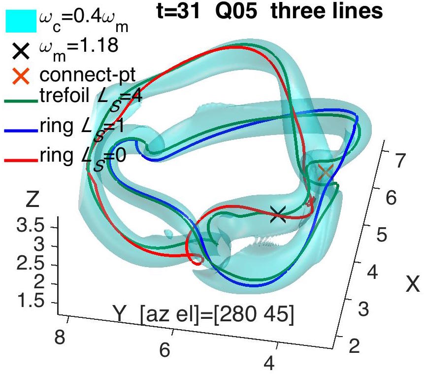
Figure 5: A single vorticity isosurface plus three closed vortex lines at $t=31$. The green line follows a remaining trefoil trajectories seeded near $\omega_{m}$, indicated by X. Its ${\cal L}_{S}=4$, split into ${\cal W+T}=2.85+1.15=4$ The orange cross is the “reconnection point”, the point between the closest approach of the trefoil’s two loops and where, due to an extra twist, the loops are locally anti-parallel. The Red ${\cal L}_{S}=0$ and blue ${\cal L}_{S}=1$ lines originate on either side of the reconnection point and are linked, which gives a total linking of ${\cal L}_{t}=2{\cal L}_{rb}+{\cal L}_{Sb}+{\cal L}_{Sr}=2+1+0=3$, the linking of the original trefoil.

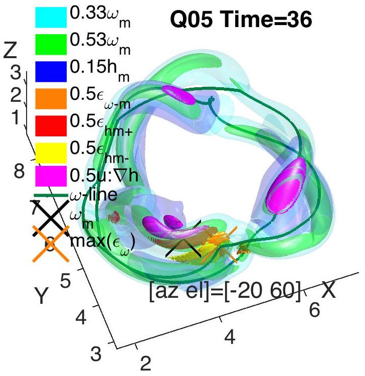
Figure 6: The perspective for $t=36$ is rotated 90^∘ clockwise from the $t=31$ figure so that the reconnection gap to the right of the orange cross and between the green $\omega$ and helicity isosurfaces can be seen directly. The vorticity isosurfaces are at $0.33\omega_{m}$ cyan and $0.53\omega_{m}$ green. The only closed trefoil line found is shown in green vortex line and helps one relate this orientation to that at $t=31$ from in figure 5. Additional isosurfaces are: blue for $h=0.15h_{m}$; orange for $0.5\epsilon_{\omega m}$=$0.5\max(\epsilon_{\omega})$ where $\max(\epsilon_{\omega})=185$; red-brown for $0.5\epsilon_{hm+}$=$0.5\max(\epsilon_{h})$ and yellow for $0.5\epsilon_{hm-}$=$0.5\min(\epsilon_{h})$, where $\max(\epsilon_{h})=4.9$ and $\min(\epsilon_{h})=-3.2$; purple for $0.5\max((\mbox{\boldmath$u$}\cdot\nabla)h)$, helicity-transport where $\max((\mbox{\boldmath$u$}\cdot\nabla)h)=0.06$. There are black and orange crosses at the positions of $\omega_{m}$ and $\max(\epsilon_{\omega})$ respectively.

Figure 7: Helicity spectra $\tilde{\cal H}_{n}=\tilde{\cal H}(k_{n})$ and $0.25\tilde{H}^{(1/2)2}_{n}$ spectra at $t=16$, 30, 54 and 60 from case Q0125. $\tilde{\cal H}_{n}<0$ values are shown in red. $0.25\tilde{H}^{(1/2)2}_{n}$ is included because it provides a guiding, but not strict, upper bound for $|\tilde{\cal H}_{n}|$ for all wavenumber shells. These particular times are shown because the $\tilde{\cal H}_{n}$ spectra are dominated by $\tilde{\cal H}_{n}>0$, the original sign of helicity, in all wavenumber shells with $k<200$ ($\log_{10}(k)\leq 2.3$) except for these two time periods. For the $16\leq t\leq 30$ time period, the period prior to the beginning of reconnection when the trefoil is rearranging itself internally, ${\cal H}_{n}<0$ spans a range of intermediate wavenumbers. This could be due to the formation of writhe of opposite polarity to the twists, twists like those along the trefoil curve in Fig. 5. The second period with $\tilde{\cal H}_{n}<0$ is represented by the spectra at $t=51$ and $t=61$, near the end of the reconnection period. At this time, $\tilde{\cal H}_{n}<0$ is dominant at the lowest wavenumbers, that is the largest physical scales.

3.4 Reconnection period in the trefoil experiment

In the discussion above it has been noted that, as in the experiments, the trefoil simulations resist reconnection and, for the higher Reynolds number cases, preserve their helicity until $t\approx 40$, which is after reconnection has begun. However, as the reconnection proceeds further, the helicity in all cases drops significantly.

It will be assumed in this discussion that the question should not be if helicity is eventually lost in the experiments, but when this occurs. Is the helicity lost during the time period the experiment covers, just after this time period, or at much later in time? This is based upon realising that eventually, as the turbulence dies, energy dissipation, $\epsilon=\nu Z$, and the enstrophy $Z$, must decrease significantly. This implies that helicity must also become decrease significantly due to the following bounds: $|{\cal H}(t)|\leq H^{(1/2)2}\leq\sqrt{2E(t)Z(t)}$. Recalling that for all time $E(t)\leq E(t=0)$.

There are several, overlapping reasons why this particular trefoil experiment is not seeing the depletion of helicity seen in the simulations, despite the similarities up to, and into, the beginning of reconnection. Possibilities include:

• The technique of identifying vortex lines from the hydrogen bubble traces is inadequate.

• The principle of multiplying the lines by the square of the original circulation to get the helicity, which is appropriate for quantised vortices and classical vortices when initialised, should not be used for classical vortices with a continuous circulation once reconnection begins.

• The timescales in the experiment have been misinterpreted.

• The topological changes reported for the experiments have been misinterpreted, possible because they have ignored how the circulation of classical vortices must reconnect gradually.

Both 1) and 2) could be issues, but because their linked ring experiment gave the expected helicity depletion, this discussion will focus upon 3) and 4).

Timescales. To be able to relate the reconnection timescale of the trefoil experiments to simulations, the trefoil simulations here and earlier work on anti-parallel and orthogonal reconnection, it is useful to give their reconnection times (when reconnection begins) in terms of their respective nonlinear timescales $t_{x}$ (16), and not in terms of $\omega_{0}^{-1}$. Thus, anti-parallel reconnection begins at about 1.75$t_{x}$ (Kerr, 2013a), orthogonal reconnection at 2.5$t_{x}$ (Kerr, 2005b) and for the the present trefoil calculations with $t_{x}=9$, reconnection begins near 3.3$t_{x}$.

This timescale argument would suggest that the experimental and numerical trefoils are not in disagreement, at least in the sense of helicity conservation until after $t\gtrsim 4t_{x}$.

Topological changes. However, Scheeler et al. (2014a) also claim that they see helicity being preserved while the trefoil reconnects first into linked rings, then into a twisted loop. While the simulations show helicity begins to decrease significantly once the trefoil has clearly begun to self-reconnect at $t=36$.

To understand these differences better, let us consider the time period during which reconnection begins in the experimental movie S4 that is accessible through Scheeler et al. (2014b) and for which they give one frame at $t=637.7$ms. This frame is from the period between their two proposed reconnections. The first is at $t\approx 625$ms, located where the twisting can be seen in the upper right in the $t=637.7$ms frame and yields the linked rings indicated by the separate orange and white trajectories. The second reconnection is at $t\approx 655$ms, with a clear gap forming roughly where the orange and white trajectories zig-zag over one another in the middle of the $t=637.7$ms frame. They say that the final configuration is a twisted loop.

However, if one compares frames from the movie at $t=614$ms and $t=661$ms, frames that represent the beginning and end of their reconnection dynamics, but do not have the orange trajectory, then the only significant change is the appearance of the gap from their second reconnection. A gap that is similar to the gap noted above for $t=36$ in figure 6.

So let us consider the following alternative scenario for this sequence of events.

• First, there is a partial reconnection at $t\approx 625$ms where some of the vortex trajectories are no longer following the original trefoil. Associated with this is the appearance of new twists along the trajectories that are not where the primary reconnection is occurring. Twists that are similar to those at $t=31$ in figure 5 near the X, but not the red X where the reconnection is actually forming.

• Only later, and not at the same location, does the true reconnection with a gap become evident. In S4 this starts at about $t=655$ms and is similar to the gap that forms in the simulations by $t=36$ in figure 6. In figure 6, the twisting around $\omega_{m}$ seen in the vortex lines at $t=31$, now manifests itself in the helicity and enstrophy dissipation terms around $\omega_{m}$.

• In the simulations all of this is considered to be one reconnection.

• This is because classical vortex reconnection is gradual. It progresses over a finite span of time and during this process twists on the edges of the reconnection event can form, twists that might look like independent reconnections. The details of this process will be described in another paper on anti-parallel reconnection.

3.5 Helicity spectra

While the physical space analysis just completed can show the basic structure of the reconnection along with the associated transport and loss of helicity, it is limited in what it can tell us about how the helicity reaches the small dissipative scales. Spectra of the energy, the helicity and their transfer spectra can fill that gap. All of these have been plotted, but only the three-dimensional spectra of the helicity ${\cal H}$ (4) and of $(H^{(1/2)})^{2}$ (8) will be shown. These spectra are constructed by accumulating the Fourier transform spectra of $\tilde{{\cal H}}(\mbox{\boldmath$k$})=\tilde{\mbox{\boldmath$u$}}(\mbox{\boldmath$k$})\cdot\tilde{\mbox{\boldmath$\omega$}}(-\mbox{\boldmath$k$})$ and $\tilde{H}^{(1/2)2}(\mbox{\boldmath$k$})=|\mbox{\boldmath$k$}||\tilde{\mbox{\boldmath$u$}}(\mbox{\boldmath$k$})|^{2}$ into three-dimensional wavenumbers shells. That is for the $(3\pi)^{3}$ with $k_{min}=2/3$ and $k_{n}=nk_{min}$:

$$\tilde{\cal H}_{n}=\sum_{k_{n}\leq|\mbox{\boldmath$k$}|\leq k_{n+1}}\tilde{{\cal H}}(\mbox{\boldmath$k$})\qquad{\rm and}\qquad\tilde{H}^{(1/2)2}_{n}=\sum_{k_{n}\leq|\mbox{\boldmath$k$}|\leq k_{n+1}}|\mbox{\boldmath$k$}||\tilde{\mbox{\boldmath$u$}}(\mbox{\boldmath$k$})|^{2}$$ (17)

The spectra will be interpreted in terms of two sets of Navier-Stokes calculations whose initial conditions were inspired by truncated shell, or dyadic, models (Biferale, 2003). In particular, how a helical spectral decomposition of the nonlinear Euler interactions (Waleffe, 1992) can be used to generate shell models with helicity-like invariants, including the popular GOY model (Biferale & Kerr, 1995). The models with the strongest interactions, and possible the strongest energy cascades, were based upon interactions between modes with oppositely signed helicity.

Part of the objective of the Navier-Stokes calculations was to determine if these interactions can ever play a significant role in the dynamics. One set of calculations used initial conditions with specified maximally helicity Fourier modes of both signs from a single mid-range wavenumber shell. Spectra showed that simultaneous cascades went to both large and small wavenumbers. Furthermore, when the higher-wavenumber cascade reached the dissipation regime and was annihilated by viscosity, large-scale helicity of the opposite sign was left behind.

This effect was studied further in Holm & Kerr (2007) who looked at both helicity spectra and the helicity on vortices in physical space. Helicity transfer spectra showed spectral pulses of helicity moving to the highest wavenumbers as twists were being generated on reconnecting vortex lines. Both the pulses and twists were then annihilated by viscosity, leaving behind helicity of the opposite sign.

Could these observations be relevant to a trefoil? A configuration whose initial helicity spectrum has only one sign. These observations could be relevant if, as the helicity re-arranges itself prior to reconnection, negative Fourier modes form. These might allow strong oppositely-signed Fourier mode interactions to form.

To demonstrate this possibility, figure 7 shows three-dimensional helicity spectra ${\cal H}_{n}$ and $0.25\tilde{H}^{(1/2)2}_{n}$ spectra from case Q00625 for two time periods, with two times shown for each period. $\tilde{\cal H}_{n}<0$ shells are in red, with the $0.25\tilde{H}^{(1/2)2}_{n}$ shells providing nearly perfect upper bounds to their absolute values $|\tilde{\cal H}|_{n}$. A version of this observation that $|{\cal H}|\leq 0.25H^{(1/2)2}$ has previously been noted for anti-parallel Euler calculations (Kerr, 2005a).

The first period uses spectra at $t=16$ and $t=30$ to represent the helicity conserving period of re-alignments just before reconnection, a period represented in physical space by figure 2 at $t=24$. The second period uses spectra at $t=54$ and $t=60$ to represent the period during which helicity is dissipated, which was represented in physical space by figure 9 at $t=63$. At low wavenumbers, the $0.25\tilde{H}^{(1/2)2}_{n}$ are all the order of $k_{n}^{-3}$, which is equivalent to $k_{n}^{-4}$ energy spectra. This $k_{n}^{-3}$ range is longer at the later times.

In the pre-reconnection period, helicity is conserved, implying that if one wavenumber shell develops either reduced or negative helicity, the helicity in another wavenumber shell must increase. Thus, at $t=16$ shells 3, 4, 5 and 6 are all negative and $0.25\tilde{H}^{(1/2)2}_{n}\sim k_{n}^{-3}$ only up to $n=4$. At $t=30$ the $\tilde{\cal H}_{n}<0$ bands are at their $0.25\tilde{H}^{(1/2)2}_{n}$ upper bound, that is more negative, with a compensating extension of the positive $k_{n}^{-3}$ to $n=6$, including with a slight hump. This transfer of positive helicity to high wavenumbers and the growth of negative helicity at intermediate wavenumbers has been confirmed by helicity transfer spectra.

For the later period, at $t=54$ there is a low wavenumber range where only one shell, $n=3$, has negative helicity. Along with its neighbouring $n=2$ and $n=4$ shells having depleted positive helicity. By $t=60$, there are two shells with $\tilde{\cal H}_{n}<0$. The helicity transfer spectra just before these times, at $t=48$ and $t=54$, show a transfer of $\tilde{\cal H}_{n}<0$ from intermediate wavenumbers to the lowest wavenumbers.

3.6 Negative helicity at large scales

Can this cascade of negative helicity to large scales be seen in physical space? First one needs to identify the direction in which the negative helicity might appear, then identify the best viewing angles. Several profiles were taken, with the $y$ profiles at $t=54$ in figure 8 indicating that the negative helicity region should be at $y\approx 8.3$. This is just outside of the envelope for $3\leq y\leq 7.5$ that contains the enstrophy.

Now that both the helicity spectra and a profile have indicated the existence of a negative helicity region at large scales for $t\sim 54$ to 60, can a $h<0$ region be found in a three-dimensional image?

Figure 9 shows that a substantial $h<0$ region does exist by using the same set of helicity+vorticity isosurfaces as in figure 2 from before reconnection. That is the same percentage of the maxima of $\omega$, $h>0$ and $h<0$, except that by $t=63$ ${\rm abs}(\min(h))$ is the same order of magnitude as ${\rm abs}(\max(h))$. Thus, a significant fraction of space now has large $h<0$.

What does the vorticity isosurface tell us about the trefoil evolution at $t=63$? By rotating the remaining blue vorticity isosurfaces alone, what remains is essentially a twisted ribbon of vorticity, consistent with the approximate self-linking number of $\tilde{{\cal L}}_{S}\approx 1$ mentioned at the end of section 3.2. Although some essense of the original trefoil does remain and because the helicity ${\cal H}$ has decayed to only 2/3rds of its original value in figure 4, one could argue that only one reconnection has benn completed. Since the graphics and $\tilde{{\cal L}}_{S}$ suggest likely that there have been two reconnections, the additional helicity is probably in the form of links whose vorticity is below the threshold of the isosurface in figure 9.

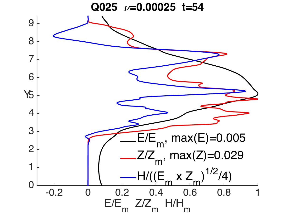
Figure 8: Helicity ${\cal H}$, energy $E$ and enstrophy $Z$ profiles in $y$ at $t=54$, normalized by their maxima, for case Q025. This time is near the end of reconnection phase and has a strong low wavenumber negative helicity ${\cal H}<0$ spectral anomaly that is similar to those in figure 7.

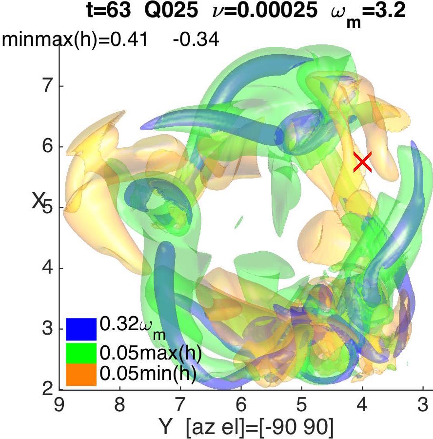
Figure 9: Isosurfaces at $t=63$ as reconnection is ending. The vorticity isosurfaces are in blue and the helicity isosurfaces are of $0.05\max(h)$ in green and $0.05\min(h)$ in yellow where $\max(h)=-0.41$ and $\min(h)=-0.34$. The position where reconnection began is indicted by the red cross.

4 Regularity

From the point of view of the phenomenology of the physics of turbulence, the reported finite $\Delta{\cal H}$ in a finite time as $\nu\rightarrow 0$ trend would make complete sense. That is, the phenomenology that inherently assumes that there is finite energy dissipation in a finite time and which underlies most of the models for turbulent dissipation used in the geophysical sciences and engineering. However, from the point of view of the current mathematics of the Navier-Stokes equations this trend cannot continue all the way to $\nu\equiv 0$.

This is referring to results that show that for any initial condition which is regular under Euler evolution up to time $t_{0}$, there exists a critical viscosity $\nu_{0}$ below which the Navier-Stokes solutions must converge to that regular Euler solution. This was originally formulated for periodic boxes (Constantin, 1986) where the definition of $\nu_{0}$ included the size of the box $\ell$. It has since been reformulated by Masmoudi (2007) in Whole Space, that is for $\ell=\infty$, so that $\nu_{0}$ can be defined solely in terms of the inverse of a function of the time integrals of the initial condition’s time-dependent Euler norms (5). This is the formulation that is relevant to these calculations because the trefoil’s volume-integrated norms are all finite as $\ell\rightarrow\infty$.

These results should apply to these trefoil calculations because the most extreme event while the trefoil evolution is still inviscid, that is before reconnetion begins, is the pre-reconnection anti-parallel re-alignment of the trefoil loops noted in figure 2 at $t=24$ and again for the trefoil trajectory in figure 5 at $t=31$. Based upon the latest evidence for Euler regularity from the series of high-resolution anti-parallel calculations in Kerr (2013b), this imples that the Euler evolution of the trefoil should also be regular.

Therefore, if the viscosity were reduced far enough below the values used here, eventually the trend for finite $-\Delta{\cal H}$ helicity loss as $\nu\rightarrow 0$ must be suppressed.

However, this result does not apply to the range of Reynolds numbers used in this paper. While the relevant time integrals of the Euler Sobolev norms have not been calculated explicitly, case R05 with a thinner initial core and larger Sobolev norms shows that $\nu>\nu_{0}$ for the larger core cases because case R05 reproduces the convergence time of the other four calculations. Which would not have been possible if $\nu\sim\nu_{0}$ applied to any of cases Q05 to Q00625,

For the ongoing high-resolution, higher Reynolds number, anti-parallel calculations that are extending those in Kerr (2013a), an explicit example will be presented for what happens to the $\nu\rightarrow 0$ trends when the $\nu\sim\nu_{0}$ threshold is crossed. And how that trend can be restored by increasing the size of the periodic box.

Figure 10: Helicity ${\cal H}$, energy $E$, $H^{(1/2)}$, $L_{3}$ and $\|\mbox{\boldmath$\omega$}\|_{\infty}$ as functions of the initial box size. Plus squares for their $t=0$ values for case R05 with a thinner core. This figure shows that for the trefoil, all of these norms have finite values in Whole Space.

5 Summary

To summarise, let us return to the three periods of evolution introduced at the beginning.

• First preservation. A long period during which the nearly maximal helicity impedes the dynamics while a locally anti-parallel alignment develops around one of the loop crossings, similar to an event observed in the experiments.

• Period at the beginning of reconnection:

  • As the reconnection begins at $t=31$ in figure 5, fragments of the original trefoil’s circulation are converted by reconnection into linking between new rings plus a twist on one of the new rings.

  • This is identified with what is called the first reconnection in the experimental movie, but for the simulations is interpreted as a region of twisting just outside the zone where the actual reconnection is beginning to form.

  • In the simulations, comparisons between the frames at $t=31$ and $t=36$ suggest that there is period of re-alignment that could be associated with the beginning of reconnection from the original trefoil into a new topology dominated by linked rings.

  • However, significant changes in the global helicity do not appear until after a true gap between reconnected vorticity isosurfaces starts to appear at $t=36$.

  • Which suggests that what is called the second reconnection in the experiment, actually represents the beginning of the first true reconnection, and only after that does the helicity start to decay. Which would have been after the last times shown in the experimental analysis.

• Later period

  • There is finite helicity dissipation in a finite time $t_{h}\approx 72$ as the viscosity goes to zero. $t_{h}$ appears to depend only upon the properties of the initial trajectory of the trefoil, the separation between of the two loops, and the trefoil’s circulation $\Gamma$.

  • Along with helicity dissipation, creation of negative helicity at the largest scales is shown in figures 7,8,9 using spectra, profiles and visualisation.

  • One way to look at this is that a closed vortex loop can generate large-scale writhe and small-scale twist, whose self-linking sum is conserved (10). This could provide a mechanism for transferring negative writhe-helicity to large scales and positive twist-helicity to the small scales. After which, the twist can break off and be dissipated, leaving behind its large-scale negative writhe-helicity.

  • Over this period the energy dissipation goes to zero as viscosity goes to zero. This is associated with only modest growth in the traditional vorticity norms.

  • It is pointed out that if only one configuration is considered, then eventually this $\nu\rightarrow 0$ trend must be suppressed for any $\nu<\nu_{0}$, where $\nu_{0}$ is a function of the Euler norms.

  • Despite this observation, this small viscosity can be decreased by using thinner initial vortices with larger Euler norms. Physically, if a given $\nu$ is too small for viscous reconnection to relieve the small-scale twisting, then by using a thinner vortex, the twisting could continue. This will the subject of later work.

6 Conclusion

The question of a dynamical role for helicity in vortex dynamics has been considered in light of recent experimental claims that helicity is preserved during the self-reconnection of trefoil vortex. Specifically, the claim is that when lines of hydrogen bubbles marking the experimental trefoil vortex knot self-reconnect that the helicity determined from the topological numbers (13) is preserved. And from this they concluded that the helicity is also preserved.

Once a perturbed initial condition for the numerical trefoil vortex knot was generated, one that was not subject to internal instabilities and did not have symmetric reconnections, both qualitative and quantitative comparisons with the experiments became possible. The first result was that as in the experiments, the helicity was preserved for a surprisingly long time. Long meaning up to and into the beginning of the first reconnection and more than 50% longer than the time for the reconnection of anti-parallel or orthogonal vortices to begin.

However, once reconnection in the simulations begins in earnest, neither the helicity nor the self-linking topological number are preserved. It is argued that the experimental conclusion in Scheeler et al. (2014a) that helicity is preserved during the trefoil reconnection is based upon how they identify the observed topological changes as coming from two reconnections. Based upon comparisons with the new simulations, these events are re-interpreted as different phases of the beginning of the first, single reconnection event. And before the helicity in the simulations begins to decay. This suggests that the true significance of the trefoil experiment, if run longer, would not only be in how it suppresses reconnection and the depletion of helicity, but in how it should also see a finite helicity dissipation in a finite rescaled time as the Reynolds number increases. Even when there is almost no energy decay.

References

- Biferale (2003) Biferale, L. 2003 Shell models of energy cascade in turbulence. Annu. Rev. Fluid Mech. 35, 441-–468.
- Biferale & Kerr (1995) Biferale, L., & Kerr, R.M. 1995 On the role of inviscid invariants in shell models of turbulence. Phys. Rev. E 52, 6113–6122.
- Calugareanu (1959) Calugareanu, G. 1959 L’intégral de Gauss et l’analyse des noeuds tridimensionels. Res. Math. Pures Appl. 4, 5–20.
- Constantin (1986) Constantin, P. 1986 Note on Loss of Regularity for Solutions of the 3—D Incompressible Euler and Related Equations. Commun. Math. Phys. 104, 311–326.
- Donzis et al. (2013) Donzis, D., Gibbon, J.D., Gupta, A., Kerr, R. M., Pandit, R., & Vincenzi., D. 2013 Vorticity moments in four numerical simulations of the 3D Navier-Stokes equations. J. Fluid Mech. 732, 316331.
- Escauriaza et al. (2003) Escauriaza, L., Seregin, G., & Sverák, V. 2003 -Solutions to the Navier-Stokes Equations and Backward Uniqueness. Russian Math. Surveys 58, 211–250. translation from Uspekhi Mat. Nauk, 58 (2003), 3–44 (Russian);
- Holm & Kerr (2007) Holm, D., & Kerr, R.M. 2007 Helicity in the formation of turbulence. Phys Fluids 19, 025101.
- Kerr (2005a) Kerr, R.M. 2005 Velocity and scaling of collapsing Euler vortices. Phys. Fluids 17, 075103.
- Kerr (2005b) Kerr, R.M. 2005 Vortex collapse and turbulence. Fluid Dyn Res 36, 249–260.
- Kerr (2013a) Kerr, R.M. 2013 Swirling, turbulent vortex rings formed from a chain reaction of reconnection events. Phys. Fluids 25, 065101.
- Kerr (2013b) Kerr, R.M. 2013 Bounds for Euler from vorticity moments and line divergence.. J. Fluid Mech. 729, R2.
- Kida & Takaoka (1987) Kida, S., & Takaoka, M. 1987 Bridging in vortex reconnection. Phys. Fluids 30, 29112914.
- Kimura & Moffatt (2014) Kimura, Y., & Moffatt, H.K. 2014 Reconnection of skewed vortices. J. Fluid Mech. 751, 329–345.
- Kleckner & Irvine (2013) Kleckner, D., & Irvine, W.T.M 2013 Creation and dynamics of knotted vortices. Nature Phys. 9, 253–258.
- Laing et al. (2015) Laing, C. E., Ricca, R.L, & Sumners, D.W.L. 2015 Conservation of writhe helicity under anti-parallel reconnection.. Sci. Rep. 5, 9224.
- Lu & Doering (2008) Lu, L., & Doering, C.R. 2008 Limits on enstrophy growth for solutions of the three-dimensional Navier-Stokes equations.. Indiana Univ. Math. J. 57, 2693.
- Masmoudi (2007) Masmoudi, N. 2007 Remarks about the inviscid limit of the Navier-Stokes system.. Commun. Math. Phys. 270, 777–788.
- Moffatt (1969) Moffatt, H.K. 1969 Degree of knottedness of tangled vortex lines. J. Fluid Mech. 35, 117–129.
- Moffatt (2014) Moffatt, H.K. 2014 and singular structures in fluid dynamics. Proc. Nat. Acad. Sci. 111, 3663–3670.
- Moffatt & Ricca (1992) Moffatt, H.K., & Ricca, R. 1992 Helicity and the Calugareanu invariant. Proc. Roy. Soc. Math. Phys. Eng. Sci. 439(1906), 411-–429.
- Orszag & Patterson (1972) Orszag, S.A., & Patterson, G.S. 1972 Numerical simulation of three-dimensional homogeneous, isotropic turbulence. Phys. Rev. Lett. 28, 7679.
- Pohl (1968) Pohl, W.F. 1968 The self-linking number of closed space curve. J. Math. Mech 17, 975–985.
- Polifke et al. (1989) Polifke, , & Shtilman, 1989 The dynamics of helical decaying turbulence. Phys. Fluids A 1, 2025–2033.
- Scheeler et al. (2014a) Scheeler, Martin W., Kleckner, Dustin, Proment, Davide, Kindlmann, Gordon L., & Irvine, William T. M. 2014 Helicity conservation by flow across scales in reconnecting vortex links and knots.. Proc. Nat. Acac. Sci. 111, 15350–15355.
- Scheeler et al. (2014b) Scheeler, Martin W., Kleckner, Dustin, Proment, Davide, Kindlmann, Gordon L., & Irvine, William T. M. Supporting information for Scheeler et al. (2014a). www.pnas.org/cgi/content/short/1407232111.
- Seregin (2011) Seregin, G.A. 2011 Necessary conditions of a potential blow-up for Navier-Stokes equations. J. Math. Sci. 178, 345–352.
- Waleffe (1992) Waleffe, F. 1992 The nature of triad interactions in homogeneous turbulence. Phys. Fluids 5, 677–685.