Factorization of the identity through operators with large diagonal

Abstract.

Given a Banach space $X$ with an unconditional basis, we consider the following question: does the identity on $X$ factor through every operator on $X$ with large diagonal relative to the unconditional basis? We show that on Gowers’ unconditional Banach space, there exists an operator for which the answer to the question is negative. By contrast, for any operator on the mixed-norm Hardy spaces $H^{p}(H^{q})$, where $1\leq p,q<\infty$, with the bi-parameter Haar system, this problem always has a positive solution. The spaces $L^{p},1<p<\infty$, were treated first by Andrew [Studia Math. 1979].

1. Introduction

Let $X$ be a Banach space. A basis for $X$ will always mean a Schauder basis. We denote by $I_{X}$ the identity operator on $X$, and write $\langle\cdot,\cdot\rangle$ for the bilinear duality pairing between $X$ and its dual space $X^{*}$. By an operator on $X$, we understand a bounded and linear mapping from $X$ into itself.

Suppose that $X$ has a normalized basis $(b_{n})_{n\in\mathbb{N}}$, and let $b_{n}^{*}\in X^{*}$ be the $n^{\text{th}}$ coordinate functional. For an operator $T$ on $X$, we say that:

• $T$ has large diagonal if $\inf_{n\in\mathbb{N}}|\langle Tb_{n},b_{n}^{*}\rangle|>0$;

• $T$ is diagonal if $\langle Tb_{m},b_{n}^{*}\rangle=0$ whenever $m,n\in\mathbb{N}$ are distinct;

• the identity operator on $X$ factors through $T$ if there are operators $R$ and $S$ on $X$ such that the diagram

  is commutative.

Suppose that the basis $(b_{n})_{n\in\mathbb{N}}$ for $X$ is unconditional. Then the diagonal operators on $X$ correspond precisely to the elements of $\ell_{\infty}(\mathbb{N})$, and so for each operator $T$ on $X$ with large diagonal, there is a diagonal operator $S$ on $X$ such that $\langle STb_{n},b_{n}^{*}\rangle=1$ for each $n\in\mathbb{N}$. This observation naturally leads to the following question.

Question 1.1.

Can the identity operator on $X$ be factored through each operator on $X$ with large diagonal?

In classical Banach spaces such as $\ell^{p}$ with the unit vector basis and $L^{p}$ with the Haar basis, the answer to this question is known to be positive. These are the theorems of Pełczyński [19] and Andrew [2], respectively; see also Johnson, Maurey, Schechtman and Tzafriri [10, Chapter 9].

The aim of the present paper is to establish the following two results.

• There exists a Banach space with an unconditional basis for which the answer to Question 1.1 is negative. This result relies heavily on the deep work of Gowers [7] and Gowers-Maurey [8].

• Question 1.1 has a positive answer for the mixed-norm Hardy space $H^{p}(H^{q})$, where $1\leq p,q<\infty$, with the bi-parameter Haar system as its unconditional basis. This conclusion can be viewed as a bi-parameter extension of Andrew’s theorem [2] on the perturbability of the one-parameter Haar system in $L^{p}$.

The precise statements of these results, together with their proofs, are given in Sections 2 and 5, respectively.

Acknowledgements

It is our pleasure to thank Th. Schlumprecht for very informative conversations and for encouraging the collaboration between Lancaster and Linz. Special thanks are due to J. B. Cooper (Linz) for drawing our attention to the work of Andrew [2].

2. The answer to Question 1.1 is not always positive

The aim of this section is to establish the following result, which answers Question 1.1 in the negative.

Theorem 2.1.

There is an operator $T$ on a Banach space $X$ with an unconditional basis such that $T$ has large diagonal, but the identity operator on $X$ does not factor through $T$.

The proof of Theorem 2.1 relies on two ingredients. The first of these is Fredholm theory, which we shall now recall the relevant parts of.

Given an operator $T$ on a Banach space $X$, we set

$$\alpha(T)=\dim\ker T\in\mathbb{N}_{0}\cup\{\infty\}\qquad\text{and}\qquad\beta(T)=\dim(X/T(X))\in\mathbb{N}_{0}\cup\{\infty\},$$

and we say that:

• $T$ is an upper semi-Fredholm operator if $\alpha(T)<\infty$ and $T$ has closed range;

• $T$ is a Fredholm operator if $\alpha(T)<\infty$ and $\beta(T)<\infty$.

Note that the condition $\beta(T)<\infty$ implies that $T$ has closed range (see, e.g., [4, Corollary 3.2.5]), so that each Fredholm operator is automatically upper semi-Fredholm. For an upper semi-Fredholm operator $T$, we define its index by

$$i(T)=\alpha(T)-\beta(T)\in\mathbb{Z}\cup\{-\infty\}.$$

The main property of the class of upper semi-Fredholm operators that we shall require is that it is stable under strictly singular perturbations in the following precise sense. Let $T$ be an upper semi-Fredholm operator on a Banach space $X$, and suppose that $S$ is an operator on $X$ which is strictly singular in the sense that, for each $\varepsilon>0$, every infinite-dimensional subspace of $X$ contains a unit vector $x$ such that $\|Sx\|\leqslant\varepsilon$. Then $T+S$ is an upper semi-Fredholm operator, and

$$i(T+S)=i(T).$$

A proof of this result can be found in [14, Proposition 2.c.10].

We shall require the following piece of notation in the proof of our next lemma. For an element $x$ of a Banach space $X$ and a functional $f\in X^{*}$, we write $x\otimes f$ for the rank-one operator on $X$ defined by

$$(x\otimes f)y=\langle y,f\rangle x\qquad(y\in X).$$

Lemma 2.2.

Let $T$ be a diagonal upper semi-Fredholm operator on a Banach space with a basis. Then $\beta(T)=\alpha(T)$, so that $T$ is a Fredholm operator with index $0$.

Proof.

Let $X$ be the Banach space on which $T$ acts, and let $(b_{n})_{n\in\mathbb{N}}$ be the basis for $X$ with respect to which $T$ is diagonal. Set $N=\{n\in\mathbb{N}:Tb_{n}=0\}$. Since $T$ is diagonal, we have $\ker T=\overline{\operatorname{span}}\{b_{n}:n\in N\}$, and so the set $N$ is finite, with $\alpha(T)$ elements. Consequently, we can define a projection of $X$ onto $\ker T$ by $P_{N}=\sum_{n\in N}b_{n}\otimes b_{n}^{*}$. The fact that $\ker P_{N}=\overline{\operatorname{span}}\{b_{n}:n\in\mathbb{N}\setminus N\}$ implies that $T(X)\subseteq\ker P_{N}$. Conversely, for each $n\in\mathbb{N}\setminus N$, we have $b_{n}=T(\langle Tb_{n},b_{n}^{*}\rangle^{-1}b_{n})$, so we conclude that $\ker P_{N}\subseteq T(X)$ because $T$ has closed range. Hence

$$\beta(T)=\dim P_{N}(X)=\alpha(T)<\infty,$$

and the result follows. ∎

The other main ingredient in the proof of Theorem 2.1 is the Banach space $X_{\text{G}}$ which Gowers [7] created to solve Banach’s hyperplane problem. This Banach space has subsequently been investigated in more detail by Gowers and Maurey [8, Section (5.1)]. Its main properties are as follows.

Theorem 2.3 (Gowers [7]; Gowers and Maurey [8]).

There is a Banach space $X_{{\text{G}}}$ with an unconditional basis such that each operator on $X_{{\text{G}}}$ is the sum of a diagonal operator and a strictly singular operator.

Corollary 2.4.

Each upper semi-Fredholm operator on the Banach space $X_{{\text{G}}}$ is a Fredholm operator of index $0$.

Proof.

Let $T$ be an upper semi-Fredholm operator on $X_{{\text{G}}}$. By Theorem 2.3, we can find a diagonal operator $D$ and a strictly singular operator $S$ on $X_{{\text{G}}}$ such that $T=D+S$. The stability of the class of upper semi-Fredholm operators under strictly singular perturbations that we stated above implies that $D$ is an upper semi-Fredholm operator with the same index as $T$, and hence the conclusion follows from Lemma 2.2. ∎

Proof of Theorem 2.1..

Let $X=X_{{\text{G}}}$ be the Banach space from Theorem 2.3, and let $(b_{n})_{n\in\mathbb{N}}$ be the unconditional basis for $X_{{\text{G}}}$ with respect to which each operator on $X_{{\text{G}}}$ is the sum of a diagonal operator and a strictly singular operator. We may suppose that $(b_{n})_{n\in\mathbb{N}}$ is normalized. Set

$$T=I_{X_{{\text{G}}}}+b_{1}\otimes b_{2}^{*}+b_{2}\otimes b_{1}^{*}.$$

Then $T$ has large diagonal because $\langle Tb_{n},b_{n}^{*}\rangle=1$ for each $n\in\mathbb{N}$.

Assume towards a contradiction that $I_{X_{{\text{G}}}}=STR$ for some operators $R$ and $S$ on $X_{{\text{G}}}$. Then $R$ is injective, and its range is complemented (because $RST$ is a projection onto it), and it is thus closed, so that $R$ is an upper semi-Fredholm operator with $\alpha(R)=0$. This implies that $R$ is a Fredholm operator of index $0$ by Corollary 2.4, and hence $R$ is invertible. Since $ST$ is a left inverse of $R$, the uniqueness of the inverse shows that $R^{-1}=ST$, but this contradicts that the operator $T$ is not injective (because $T(b_{1}-b_{2})=0$). ∎

As we have seen in the proof of Theorem 2.1, the identity operator need not factor through a Fredholm operator. If, however, we allow ourselves sums of two operators, then we can always factor the identity operator, as the following result shows.

Proposition 2.5.

Let $T$ be a Fredholm operator on an infinite-dimensional Banach space $X$. Then there are operators $R_{1}$, $R_{2}$, $S_{1}$, and $S_{2}$ on $X$ such that

$$I_{X}=S_{1}TR_{1}+S_{2}TR_{2}.$$

Proof.

Let $P=\sum_{j=1}^{n}x_{j}\otimes f_{j}$ be a projection of $X$ onto the kernel of $T$, where $n\in\mathbb{N}$, $x_{1},\ldots,x_{n}\in X$, and $f_{1},\ldots,f_{n}\in X^{*}$, and let $Q$ be a projection of $X$ onto the range of $T$. Since this range is infinite-dimensional, we can find $y_{1},\ldots,y_{n}\in X$ and $g_{1},\ldots,g_{n}\in X^{*}$ such that $\langle Ty_{j},g_{k}\rangle=\delta_{j,k}$ (the Kronecker delta) for each $j,k\in\{1,\ldots,n\}$. The restriction $\widetilde{T}\colon x\mapsto Tx,\,\ker P\to T(X)$, is invertible, so we may define an operator on $X$ by $S_{1}=J\widetilde{T}^{-1}Q$, where $J\colon\ker P\to X$ is the inclusion. Set

$$R_{1}=I_{X}-P,\qquad R_{2}=\sum_{j=1}^{n}y_{j}\otimes f_{j},\qquad\text{and}\qquad S_{2}=\sum_{k=1}^{n}x_{k}\otimes g_{k}.$$

Then, for each $z\in X$, we have

$$(S_{1}TR_{1}+S_{2}TR_{2})z =J\widetilde{T}^{-1}QT(z-Pz)+\sum_{j,k=1}^{n}\langle Ty_{j},g_{k}\rangle\langle z,f_{j}\rangle x_{k}$$

$$=(z-Pz)+Pz=z,$$

from which the conclusion follows. ∎

3. The answer to Question 1.1 is positive in mixed-norm Hardy spaces

In many classical Banach spaces, the answer to Question 1.1 is known to be positive. This includes $\ell^{p}$, $p\geq 1$, and $L^{p}$, $p>1$, see Pełczyński [19] and Andrew [2], respectively. Closely related to this question is the work of Johnson, Maurey, Schechtman and Tzafriri [10, Chapter 9], in which they specify a criterion for an operator on a rearrangement invariant function space to be a factor of the identity.

We now turn to defining the mixed-norm Hardy spaces together with an unconditional basis, the bi-parameter Haar system. Let $\mathscr{D}$ denote the collection of dyadic intervals given by

$$\mathscr{D}=\{[k2^{-n},(k+1)2^{-n})\,:\,n,k\in\mathbb{N}_{0},0\leq k\leq 2^{n}-1\}.$$

The dyadic intervals are nested, i.e. if $I,J\in\mathscr{D}$, then $I\cap J\in\{I,J,\emptyset\}$. For $I\in\mathscr{D}$ we let $|I|$ denote the length of the dyadic interval $I$. Let $I\in\mathscr{D}$ and $I\neq[0,1)$, then $\widetilde{I}$ is the unique dyadic interval satisfying $\widetilde{I}\supset I$ and $|\widetilde{I}|=2|I|$. Given $N_{0}\in\mathbb{N}_{0}$ we define

$$\mathscr{D}_{N_{0}}=\{I\in\mathscr{D}\,:\,|I|=2^{-N_{0}}\}\qquad\text{and}\qquad\mathscr{D}^{N_{0}}=\{I\in\mathscr{D}\,:\,|I|\geq 2^{-N_{0}}\}.$$

Let $h_{I}$ be the $L^{\infty}$-normalized Haar function supported on $I\in\mathscr{D}$; that is, for $I=[a,b)$ and $c=(a+b)/2$, we have $h_{I}(x)=1$ if $a\leq x<c$, $h_{I}(x)=-1$ if $c\leq x<b$, and $h_{I}(x)=0$ otherwise. Moreover, let $\mathscr{R}=\{I\times J:I,J\in\mathscr{D}\}$ be the collection of dyadic rectangles contained in the unit square, and set

$$h_{I\times J}(x,y)=h_{I}(x)h_{J}(y),\qquad(I\times J\in\mathscr{R},\,x,y\in[0,1)).$$

For $1\leq p,q<\infty$, the mixed-norm Hardy space $H^{p}(H^{q})$ is the completion of

$$\operatorname{span}\{h_{I\times J}\,:\,I\times J\in\mathscr{R}\}$$

under the square function norm

$$\|f\|_{H^{p}(H^{q})}=\bigg{(}\int_{0}^{1}\Big{(}\int_{0}^{1}\big{(}\sum_{I\times J}|a_{I\times J}|^{2}h_{I\times J}^{2}(x,y)\big{)}^{q/2}\,\mathrm{d}y\Big{)}^{p/q}\,\mathrm{d}x\bigg{)}^{1/p},$$ (3.1)

where $f=\sum_{I\times J}a_{I\times J}h_{I\times J}$. Then $(h_{I\times J})_{I\times J\in\mathscr{R}}$ is a $1$-unconditional basis of $H^{p}(H^{q})$, called the bi-parameter Haar system. We begin with the following facts:

• It is recorded by Capon [3] that the identity operator provides an isomorphism between $H^{p}(H^{q})$ and $L^{p}(L^{q})$, $1<p,q<\infty$.

• Since the bi-parameter Haar system $\{h_{I\times J}:I\times J\in\mathscr{R}\}$ is an unconditional basis, we do not need to specify an ordering of its index set $\mathscr{R}$.

• This basis is $L^{\infty}$-normalized and not normalized in $H^{p}(H^{q})$; we have

  $$\|h_{I\times J}\|_{H^{p}(H^{q})}=|I|^{1/p}|J|^{1/q}.$$

An operator $T\,:\,H^{p}(H^{q})\to H^{p}(H^{q})$ has large diagonal with respect to the $L^{\infty}$-normalized Haar system $\{h_{I\times J}:I\times J\in\mathscr{R}\}$ if and only if for some $\delta>0$ we have that $|\langle Th_{I\times J},h_{I\times J}\rangle|\geq\delta|I\times J|$ for all $I\times J\in\mathscr{R}$. The remaining sections of the paper are devoted to proving the following theorem.

Theorem 3.1.

Let $1\leq p,q<\infty$ and $\delta>0$, and let $T:H^{p}(H^{q})\to H^{p}(H^{q})$ be an operator satisfying

$$|\langle Th_{I\times J},h_{I\times J}\rangle|\geq\delta|I\times J|\qquad\text{for all $I\times J\in\mathscr{R}$}.$$

Then the identity operator on $H^{p}(H^{q})$ factors through $T$, that is, there are operators $R$ and $S$ such that the diagram

(3.2)

is commutative. Moreover, for any $\eta\in(0,1]$ the operators $R$ and $S$ can be chosen such that $\|R\|\|S\|\leq(1+\eta)/\delta$.

For related, local (finite dimensional, quantitative) factorization theorems in bi-parameter $H^{1}$ and BMO, see [18, 13]. Recently in [11], the second named author obtained local factorization results in mixed-norm Hardy and BMO spaces by combining methods of the present paper with techniques of [13]. Despite the fact that the constants in our theorem are independent of $p$ and $q$, we remark that the passage to the non-separable limiting spaces (corresponding to $p=\infty$ or $q=\infty$) cannot be deduced routinely from the proof given below. The non-separable space $SL^{\infty}$ consisting of functions with square function in $L^{\infty}$ would be an example of such a limiting space. Factorization theorems in $SL^{\infty}$ are treated by the second named author in [12].

The cornerstones upon which the constructions of the operators $R,S$ in Theorem 3.1 rest are embeddings and projections onto a carefully chosen block basis of the bi-parameter Haar system in mixed-norm Hardy spaces.

4. Capon’s local product condition and its consequences

In this section, we treat embeddings and projections in $H^{p}(H^{q})$. They are the main pillars of the construction underlying the proof of Theorem 3.1. We begin by listing some elementary and well known facts concerning $H^{p}(H^{q})$ and its dual.

4.1. Basic facts and notation

Let $1\leq p,q<\infty$ and let $H^{p}(H^{q})^{*}$ denote the dual space of $H^{p}(H^{q})$, identified as a space of functions on $[0,1)^{2}$. Then the duality pairing between $H^{p}(H^{q})$ and $H^{p}(H^{q})^{*}$ is given by

$$\langle f,g\rangle=\int_{0}^{1}\int_{0}^{1}f(x,y)g(x,y)\,\mathrm{d}y\,\mathrm{d}x.$$

Correspondingly, we have

$$\|g\|_{H^{p}(H^{q})^{*}}=\sup_{\|f\|_{H^{p}(H^{q})}\leq 1}|\langle f,g\rangle|.$$

Since $h_{I\times J}$, $I\times J\in\mathscr{R}$ is a $1$-unconditional Schauder basis in $H^{p}(H^{q})$, we may identify an element $g\in H^{p}(H^{q})^{*}$ with the sequence $(\langle h_{I\times J},g\rangle)_{I\times J}$. In the dual space, the norm of $(|\langle h_{I\times J},g\rangle|)_{I\times J}$ is equal to the norm of $(\langle h_{I\times J},g\rangle)_{I\times J}$. See [14, Chapter 1].

If $1<p,p^{\prime},q,q^{\prime}<\infty$ and $\frac{1}{p}+\frac{1}{p^{\prime}}=1$, $\frac{1}{q}+\frac{1}{q^{\prime}}=1$, it is recorded by Capon [3] that there is a constant $C_{p,q}$ such that for any finite linear combination $f$ of Haar functions we have

$$C_{p,q}^{-1}\|f\|_{L^{p}(L^{q})}\leq\|f\|_{H^{p}(H^{q})}\leq C_{p,q}\|f\|_{L^{p}(L^{q})}.$$

Consequently, the identity operator provides an isomorphism between $H^{p}(H^{q})$ and $L^{p}(L^{q})$, and the dual of $H^{p}(H^{q})$ identifies with $H^{p^{\prime}}(H^{q^{\prime}})$. Capon’s argument is based on the observation by Pisier that the $\text{UMD}_{p}$ property of a Banach space does not depend on the value of $1<p<\infty$. For a proof of Pisier’s observation, we refer to [15] respectively [20, Chapter 5].

For the limiting cases we have $H^{1}(H^{q})^{*}=\text{BMO}(H^{q^{\prime}})$, $H^{p}(H^{1})^{*}=H^{p^{\prime}}(\text{BMO})$ and $H^{1}(H^{1})^{*}=\text{BMO}(\text{BMO})$. See Maurey [16] and Müller [17].

Let $\{\mathscr{B}_{R}:R\in\mathscr{R}\}$ be a pairwise disjoint family, where each set $\mathscr{B}_{R}$ is a finite collection of disjoint dyadic rectangles. Given a vector of scalars $\beta=(\beta_{R}:R\in\bigcup_{Q\in\mathscr{R}}\mathscr{B}_{Q})$, we define

$$b_{R}^{(\beta)}(x,y)=\sum_{Q\in\mathscr{B}_{R}}\beta_{Q}h_{Q}(x,y),\qquad x,y\in[0,1)$$ (4.1)

and we call $\{b_{R}^{(\beta)}:R\in\mathscr{R}\}$ the block basis generated by $\{\mathscr{B}_{R}:R\in\mathscr{R}\}$ and $\beta=(\beta_{R}:R\in\bigcup_{Q\in\mathscr{R}}\mathscr{B}_{Q})$. Now, let $1\leq p,q<\infty$ be fixed. Note that $\{b_{R}^{(\beta)}:R\in\mathscr{R}\}$ is $1$-unconditional in $H^{p}(H^{q})$ since $\{h_{R}:R\in\mathscr{R}\}$ is $1$-unconditional in $H^{p}(H^{q})$, i.e.

$$\Big{\|}\sum_{R\in\mathscr{R}}\gamma_{R}\alpha_{R}b_{R}^{(\beta)}\Big{\|}_{H^{p}(H^{q})}\leq\sup_{R\in\mathscr{R}}|\gamma_{R}|\ \Big{\|}\sum_{R\in\mathscr{R}}\alpha_{R}b_{R}^{(\beta)}\Big{\|}_{H^{p}(H^{q})},\qquad(\gamma_{R})_{R\in\mathscr{R}}\in\ell^{\infty}(\mathscr{R}),$$

whenever the series $\sum_{R\in\mathscr{R}}\alpha_{R}b_{R}^{(\beta)}$ converges. We say that the system $\{b_{R}^{(\beta)}:R\in\mathscr{R}\}$ is equivalent to the Haar system $\{h_{R}:R\in\mathscr{R}\}$ if the operator $B_{\beta}:H^{p}(H^{q})\to H^{p}(H^{q})$ given by

$$B_{\beta}(f)=\sum_{R\in\mathscr{R}}\frac{\langle f,h_{R}\rangle}{\|h_{R}\|_{2}^{2}}\,b_{R}^{(\beta)},\qquad f\in H^{p}(H^{q}),$$

is bounded and an isomorphism onto its range. In this case, whenever $C_{1},C_{2}>0$ are constants such that

$$\frac{1}{C_{1}}\|f\|_{H^{p}(H^{q})}\leq\|B_{\beta}f\|_{H^{p}(H^{q})}\leq C_{2}\|f\|_{H^{p}(H^{q})},\qquad f\in H^{p}(H^{q}),$$

we say that $\{b_{R}^{(\beta)}:R\in\mathscr{R}\}$ is $C_{1}C_{2}$-equivalent to $\{h_{R}:R\in\mathscr{R}\}$.

If $\beta_{R}=1$ for each $R\in\mathscr{R}$, then we write $b_{R}$ instead of $b_{R}^{(\beta)}$ and $B$ in place of $B_{\beta}$.

4.2. Uniform weak and weak* limits

Let $\Gamma$ denote the closed unit ball of $\ell^{\infty}(\mathscr{R})$, so that $\Gamma$ consists of all families $\gamma=(\gamma_{R}:R\in\mathscr{R})$ of scalars with $|\gamma_{R}|\leq 1$ for each $R\in\mathscr{R}$. Given $\gamma\in\Gamma$, the $1$-unconditionality of the bi-parameter Haar system implies that the definition

$$M_{\gamma}\colon h_{R}\mapsto\gamma_{R}h_{R},\qquad R\in\mathscr{R}$$ (4.2)

extends uniquely to an operator of norm $\sup_{R}|\gamma_{R}|$ on $H^{p}(H^{q})$.

Lemma 4.1.

For $m\in\mathbb{N}$, let $\mathscr{X}_{m}$ and $\mathscr{Y}_{m}$ be non-empty, finite families of pairwise disjoint dyadic intervals, define $f_{m}=\sum_{I\in\mathscr{X}_{m},\,J\in\mathscr{Y}_{m}}h_{I\times J}$, $X_{m}=\bigcup\mathscr{X}_{m}$, and $Y_{m}=\bigcup\mathscr{Y}_{m}$, and let $1\leq p,q<\infty$. Then:

1. $\|f_{m}\|_{H^{p}(H^{q})}=|X_{m}|^{1/p}|Y_{m}|^{1/q}$ for all $m\in\mathbb{N}$;

2. $\|f_{m}\|_{H^{p}(H^{q})^{*}}=|X_{m}|^{1-1/p}|Y_{m}|^{1-1/q}$ for all $m\in\mathbb{N}$.

Suppose in addition that:

• $\mathscr{X}_{m}\cap\mathscr{X}_{n}=\emptyset$ or $\mathscr{Y}_{m}\cap\mathscr{Y}_{n}=\emptyset$ whenever $m,n\in\mathbb{N}$ are distinct;

• $X_{m}=X_{n}$ and $Y_{m}=Y_{n}$ for all $m,n\in\mathbb{N}$.

Then:

1. the sequence $(|X_{m}|^{-1/p}|Y_{m}|^{-1/q}f_{m})_{m\in\mathbb{N}}$ in $H^{p}(H^{q})$ is isometrically equivalent to the unit vector basis of $\ell^{2}$;

2. for each $g\in H^{p}(H^{q})^{*}$, $\sup_{\gamma\in\Gamma}|\langle M_{\gamma}f_{m},g\rangle|\to 0$ as $m\to\infty$;

3. for each $g\in H^{p}(H^{q})$, $\sup_{\gamma\in\Gamma}|\langle M_{\gamma}g,f_{m}\rangle|\to 0$ as $m\to\infty$.

Note that in (i), (iii), and (iv), we regard $f_{m}$ as an element of $H^{p}(H^{q})$, whereas in (ii) and (v), we regard it as an element of $H^{p}(H^{q})^{*}$.

Proof.

Set $\mathscr{B}_{m}=\{I\times J:I\in\mathscr{X}_{m},\,J\in\mathscr{Y}_{m}\}$ for each $m\in\mathbb{N}$.

(i). This follows immediately from the definition of $\|\cdot\|_{H^{p}(H^{q})}$.

(ii). For any $g=\sum_{K\times L\in\mathscr{B}_{m}}a_{K\times L}h_{K\times L}\in H^{p}(H^{q})$ we obtain by Hölder’s inequality that

$$|\langle f_{m},g\rangle| \leq\sum_{K\in\mathscr{X}_{m}}|K|\sum_{L\in\mathscr{Y}_{m}}|a_{K\times L}||L|\leq|Y_{m}|^{1-1/q}\sum_{K\in\mathscr{X}_{m}}|K|\Bigl{(}\sum_{L\in\mathscr{Y}_{m}}|a_{K\times L}|^{q}|L|\Bigr{)}^{1/q}$$

$$\leq|X_{m}|^{1-1/p}|Y_{m}|^{1-1/q}\biggl{(}\sum_{K\in\mathscr{X}_{m}}|K|\Bigl{(}\sum_{L\in\mathscr{Y}_{m}}|a_{K\times L}|^{q}|L|\Bigr{)}^{p/q}\biggr{)}^{1/p}$$

$$=|X_{m}|^{1-1/p}|Y_{m}|^{1-1/q}\|g\|_{H^{p}(H^{q})},$$

and thus we have proved $\|f_{m}\|_{H^{p}(H^{q})^{*}}\leq|X_{m}|^{1-1/p}|Y_{m}|^{1-1/q}$. For the other inequality, recall from (i) that $\|f_{m}\|_{H^{p}(H^{q})}=|X_{m}|^{1/p}|Y_{m}|^{1/q}$, thus

$$\langle f_{m},f_{m}\rangle=|X_{m}||Y_{m}|=|X_{m}|^{1-1/p}|Y_{m}|^{1-1/q}\|f_{m}\|_{H^{p}(H^{q})}.$$

(iii). We observe that the first of the additional assumptions ensures that $\mathscr{B}_{m}\cap\mathscr{B}_{n}=\emptyset$ whenever $m,n\in\mathbb{N}$ are distinct. Set $X:=X_{m}$ and $Y:=Y_{m}$ for some (and hence all) $m\in\mathbb{N}$, and let $(c_{m})_{m\in\mathbb{N}}$ be a sequence of scalars that vanishes eventually. Since

$$\sum_{R\in\mathscr{B}_{m}}{\mathbbm{1}}_{R}(x,y)=\Bigl{(}\sum_{I\in\mathscr{X}_{m}}{\mathbbm{1}}_{I}(x)\Bigr{)}\Bigl{(}\sum_{J\in\mathscr{Y}_{m}}{\mathbbm{1}}_{J}(y)\Bigr{)}={\mathbbm{1}}_{X}(x){\mathbbm{1}}_{Y}(y)$$

for all $m\in\mathbb{N}$ and $x,y\in[0,1)$, (3.1) implies that

$$\Bigl{\|}\sum_{m}c_{m}f_{m}\Bigr{\|}_{H^{p}(H^{q})}^{p} =\int_{0}^{1}\biggl{(}\int_{0}^{1}\Bigl{(}\sum_{m}|c_{m}|^{2}{\mathbbm{1}}_{X}(x){\mathbbm{1}}_{Y}(y)\Bigr{)}^{q/2}\mathrm{d}y\biggr{)}^{p/q}\mathrm{d}x$$

$$=\Bigl{(}\sum_{m}|c_{m}|^{2}\Bigr{)}^{p/2}|X|\,|Y|^{p/q},$$

from which the conclusion follows.

(iv). Let $g\in H^{p}(H^{q})^{*}$ and $\varepsilon>0$. For each $R\in\mathscr{R}$, we can choose a scalar $\beta_{R}$ with $|\beta_{R}|=1$ such that $\beta_{R}\langle h_{R},g\rangle=|\langle h_{R},g\rangle|$. Set $\beta=(\beta_{R})\in\Gamma$. By (iii), the sequence $(f_{m})_{m\in\mathbb{N}}$ converges weakly to $0$, so we can find $m_{0}\in\mathbb{N}$ such that $|\langle f_{m},M_{\beta}^{*}g\rangle|\leq\varepsilon$ whenever $m\geq m_{0}$. Then, for each $\gamma=(\gamma_{R})\in\Gamma$ and $m\geq m_{0}$ we have

$$|\langle M_{\gamma}f_{m},g\rangle| =\Bigl{|}\sum_{R\in\mathscr{B}_{m}}\gamma_{R}\langle h_{R},g\rangle\Bigr{|}\leq\sum_{R\in\mathscr{B}_{m}}|\langle h_{R},g\rangle|$$

$$=\sum_{R\in\mathscr{B}_{m}}\beta_{R}\langle h_{R},g\rangle=\langle M_{\beta}f_{m},g\rangle\leq\varepsilon,$$

as required.

(v). Given $g\in H^{p}(H^{q})$ and $\varepsilon>0$, we choose a finite subset $\mathscr{F}$ of $\mathscr{R}$ such that $\|g-Pg\|_{H^{p}(H^{q})}\leq\varepsilon$, where $P:H^{p}(H^{q})\to H^{p}(H^{q})$ is the orthogonal projection given by $Pf=\sum_{R\in\mathscr{F}}\frac{\langle f,h_{R}\rangle}{|R|}h_{R}$. Since the sets $\mathscr{B}_{m},\,m\in\mathbb{N}$, are pairwise disjoint and $\mathscr{F}$ is finite, we can find $m_{0}\in\mathbb{N}$ such that $\bigl{(}\bigcup_{m\geq m_{0}}\mathscr{B}_{m}\bigr{)}\cap\mathscr{F}=\emptyset$. Then, for each $m\geq m_{0}$ and $\gamma\in\Gamma$, we have $P^{*}f_{m}=0$, and hence

$$|\langle M_{\gamma}g,f_{m}\rangle| =|\langle M_{\gamma}g,(I-P)^{*}f_{m}\rangle|=|\langle M_{\gamma}(I-P)g,f_{m}\rangle|$$

$$\leq\|M_{\gamma}\|\,\|g-Pg\|_{H^{p}(H^{q})}\|f_{m}\|_{H^{p}(H^{q})^{*}}\leq\varepsilon,$$

where we have used that $M_{\gamma}$ commutes with $P$, and that

$$\|f_{m}\|_{H^{p}(H^{q})^{*}}=|X|^{1-1/p}|Y|^{1-1/q}\leq 1$$

by (ii). ∎

4.3. Embeddings and projections

For each $R\in\mathscr{R}$ let $\mathscr{X}_{R},\mathscr{Y}_{R}\subset\mathscr{D}$ denote non-empty, finite collections of dyadic intervals that define the collection of dyadic rectangles $\mathscr{B}_{R}$ by

$$\mathscr{B}_{R}=\{K\times L\,:\,K\in\mathscr{X}_{R},\,L\in\mathscr{Y}_{R}\},\qquad R\in\mathscr{R}.$$ (4.3)

Now (4.1) assumes the following form, if $\beta_{R}=1$ for each $R\in\mathscr{R}$:

$$b_{R}(x,y)=\Big{(}\sum_{K\in\mathscr{X}_{R}}h_{K}(x)\Big{)}\Big{(}\sum_{L\in\mathscr{Y}_{R}}h_{L}(y)\Big{)},\qquad R\in\mathscr{R};$$ (4.4)

see Figure 1.

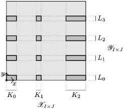
Figure 1. For a dyadic rectangle $I\times J\in\mathscr{R}$, this figure depicts $\mathscr{B}_{I\times J}=\mathscr{X}_{I\times J}\times\mathscr{Y}_{I\times J}$ (the collection of the dark gray rectangles) contained in the unit square (the light gray area). Here, $\mathscr{X}_{I\times J}=\{K_{0},K_{1},K_{2}\}$. The dyadic rectangles in $K_{i}\times\mathscr{Y}_{I\times J}$ are connected by dotted lines.

Capon [3] discovered a condition for $\{\mathscr{B}_{R}:R\in\mathscr{R}\}$ which ensures that the block basis $\{b_{R}:R\in\mathscr{R}\}$ given by (4.4) is equivalent to the Haar system $\{h_{R}:R\in\mathscr{R}\}$ in $H^{p}(H^{q})$, whenever $1<p,q<\infty$ (see Theorem 4.2). The local product condition (P1)–(P4) has its roots in Capon’s seminal work [3].

We now introduce some notation. For $R\in\mathscr{R}$ we set

$$X_{R}=\bigcup\{K:K\in\mathscr{X}_{R}\}\qquad\text{and}\qquad Y_{R}=\bigcup\{L:L\in\mathscr{Y}_{R}\}.$$ (4.5)

For each $I_{0}\times J_{0}\in\mathscr{R}$ we consider the following unions

$$X_{I_{0}}=\bigcup\{X_{I_{0}\times J}:J\in\mathscr{D}\},\quad Y_{J_{0}}=\bigcup\{Y_{I\times J_{0}}:I\in\mathscr{D}\}.$$ (4.6)

Clearly, for all $I\times J\in\mathscr{R}$ the following crucial inclusions hold true:

$$X_{I\times J}\subset X_{I}\qquad\text{and}\qquad Y_{I\times J}\subset Y_{J}.$$ (4.7)

We say that $\{\mathscr{B}_{I\times J}:I\times J\in\mathscr{R}\}$ given by (4.3) satisfies the local product condition with constants $C_{X},C_{Y}>0$, if the following four properties (P1), (P2), (P3) and (P4) hold true.

1. For all $R\in\mathscr{R}$ the collection $\mathscr{B}_{R}$ consists of pairwise disjoint dyadic rectangles, and for all $R_{0},R_{1}\in\mathscr{R}$ with $R_{0}\neq R_{1}$ we have $\mathscr{B}_{R_{0}}\operatorname{\cap}\mathscr{B}_{R_{1}}=\emptyset$.

2. For all $I\times J,I_{0}\times J_{0},I_{1}\times J_{1}\in\mathscr{R}$ with $I_{0}\cap I_{1}=\emptyset$, $I_{0}\operatorname{\cup}I_{1}\subset I$ and $J_{0}\cap J_{1}=\emptyset$, $J_{0}\operatorname{\cup}J_{1}\subset J$ we have

   $$X_{I_{0}}\operatorname{\cap}X_{I_{1}} =\emptyset, X_{I_{0}}\operatorname{\cup}X_{I_{1}} \subset X_{I},$$

   $$Y_{J_{0}}\operatorname{\cap}Y_{J_{1}} =\emptyset, Y_{J_{0}}\operatorname{\cup}Y_{J_{1}} \subset Y_{J}.$$

3. For each $R=I\times J\in\mathscr{R}$, we have

   $$|I|\leq C_{X}|X_{R}|,\qquad|X_{I}|\leq C_{X}|I|,\qquad|J|\leq C_{Y}|Y_{R}|,\qquad|Y_{J}|\leq C_{Y}|J|.$$

4. For all $I_{0}\times J_{0},I\times J\in\mathscr{R}$ with $I_{0}\times J_{0}\subset I\times J$ and for every $K\in\mathscr{X}_{I\times J}$ and $L\in\mathscr{Y}_{I\times J}$, we have

   $$\frac{|K\operatorname{\cap}X_{I_{0}}|}{|K|}\geq C_{X}^{-1}\frac{|X_{I_{0}}|}{|X_{I}|}\qquad\text{and}\qquad\frac{|L\operatorname{\cap}Y_{J_{0}}|}{|L|}\geq C_{Y}^{-1}\frac{|Y_{J_{0}}|}{|Y_{J}|}.$$

See Figure 2 for the collections $\mathscr{X}_{R}$, $R\in\mathscr{R}$, and Figure 3 as well as Figure 4 for a depiction of $\mathscr{X}_{R}$ and $\mathscr{Y}_{R}$, $R\in\mathscr{R}$.

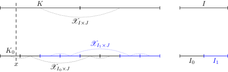
Figure 2. The figure depicts the collections $\mathscr{X}_{I\times J}$, $\mathscr{X}_{I_{0}\times J}$, $\mathscr{X}_{I_{1}\times J}$, with $I_{0}\operatorname{\cup}I_{1}=I$ and $I_{0}\cap I_{1}=\emptyset$, $J\in\mathscr{D}$. Given $x\in[0,1)$, the dashed vertical line connects the intervals $K_{0}$ and $K$ with $x\in K_{0}\subset K$. By (P2) we have $X_{I_{0}}\subset X_{I}$, and in the figure (P4) is realized by $\frac{|K\operatorname{\cap}X_{I_{0}}|}{|K|}=\frac{|X_{I_{0}}|}{|X_{I}|}$.

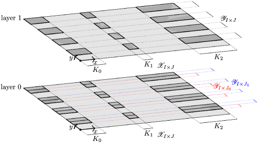
Figure 3. The dyadic rectangles $I\times J$, $I\times J_{0}$ and $I\times J_{1}$ in $\mathscr{R}$ are such that $J_{0}\operatorname{\cup}J_{1}=J$ and $J_{0}\cap J_{1}=\emptyset$. This figure depicts the collections $\mathscr{B}_{I\times J}=\mathscr{X}_{I\times J}\times\mathscr{Y}_{I\times J}$ in the top layer, and $\mathscr{B}_{I\times J_{0}}=\mathscr{X}_{I\times J_{0}}\times\mathscr{Y}_{I\times J_{0}}$ and $\mathscr{B}_{I\times J_{1}}=\mathscr{X}_{I\times J_{1}}\times\mathscr{Y}_{I\times J_{1}}$ in the bottom layer. Here, $\mathscr{X}_{I\times J}=\mathscr{X}_{I_{0}\times J}=\mathscr{X}_{I_{1}\times J}=\{K_{0},K_{1},K_{2}\}$. Each interval in $\mathscr{Y}_{I\times J}$ is split in two intervals, which are then placed into $\mathscr{Y}_{I\times J_{0}}$ and $\mathscr{Y}_{I\times J_{1}}$, respectively.

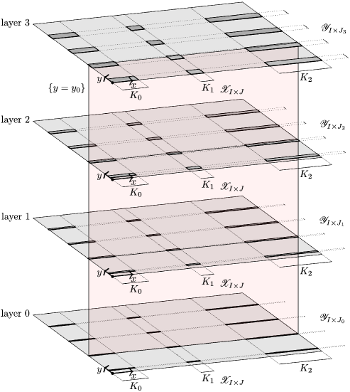
Figure 4. In the figure, $\mathscr{X}_{I\times J_{j}}=\{K_{0},K_{1},K_{2}\}$, $0\leq j\leq 3$, whereas $\mathscr{Y}_{I\times J_{j}}$ changes with each layer $0\leq j\leq 3$. For $y_{0}\in[0,1)$, the light red vertical plane connects the lines $\ell=\{(x,y_{0}):x\in[0,1)\}$ in the four layers depicted in the figure.

Theorem 4.2 (Capon).

Let $1\leq p,q<\infty$. If the conditions (P1)–(P3) are satisfied, then $\{b_{I\times J}\,:\,I\times J\in\mathscr{R}\}$ is $C$-equivalent to $\{h_{I\times J}\,:\,I\times J\in\mathscr{R}\}$ in $H^{p}(H^{q})$, where $C$ depends only on $C_{X}$ and $C_{Y}$.

We emphasize that $p$ or $q$ may take the value $1$ in the above theorem. By a duality argument, M. Capon [3] showed the equivalence stated in Theorem 4.2 implies that the orthogonal projection $P\,:\,H^{p}(H^{q})\to H^{p}(H^{q})$ given by

$$Pf=\sum_{I\times J\in\mathscr{R}}\frac{\langle f,b_{I\times J}\rangle}{\|b_{I\times J}\|_{2}^{2}}b_{I\times J}$$ (4.8)

is bounded on $H^{p}(H^{q})$, whenever $1<p,q<\infty$. We point out that the parameters $p=1$ or $q=1$ are both excluded by the duality argument. Indeed, the duality argument of Capon shows that

$$\|P:H^{p}(H^{q})\to H^{p}(H^{q})\|\leq C(p,q,C_{X},C_{Y}),$$

where the constants $C(p,q,C_{X},C_{Y})\to\infty$ in each of the cases $p\to 1$, $p\to\infty$, $q\to 1$ or $q\to\infty$.

The next theorem is our first major step towards proving Theorem 3.1. We show that the operator $P$ is bounded on $H^{p}(H^{q})$, $1\leq p,q<\infty$ with an upper estimate for the norm independent of $p$ or $q$. Specifically, Theorem 4.3 includes the cases $p=1$ or $q=1$.

Theorem 4.3.

Let $1\leq p,q<\infty$, let $\{\mathscr{B}_{R}\,:\,R\in\mathscr{R}\}$ be a pairwise disjoint family which satisfies the local product condition (P1)–(P4) with constants $C_{X}$ and $C_{Y}$, and let $\beta=(\beta_{Q}:Q\in\bigcup_{R\in\mathscr{R}}\mathscr{B}_{R})$ be a family of scalars such that

$$M:=\sup_{Q}|\beta_{Q}|<\infty.$$

Then the operators $B_{\beta},A_{\beta}:H^{p}(H^{q})\to H^{p}(H^{q})$ given by

$$B_{\beta}f=\sum_{R\in\mathscr{R}}\frac{\langle f,h_{R}\rangle}{\|h_{R}\|_{2}^{2}}b_{R}^{(\beta)}\qquad\text{and}\qquad A_{\beta}f=\sum_{R\in\mathscr{R}}\frac{\langle f,b_{R}^{(\beta)}\rangle}{\|b_{R}\|_{2}^{2}}h_{R}$$

satisfy the estimates

$$\|B_{\beta}f\|_{H^{p}(H^{q})} \leq MC_{X}^{1/p}C_{Y}^{1/q}\|f\|_{H^{p}(H^{q})}, f \in H^{p}(H^{q}),$$ (4.9)

$$\|A_{\beta}f\|_{H^{p}(H^{q})} \leq MC_{X}^{3+1/p}C_{Y}^{3+1/q}\|f\|_{H^{p}(H^{q})}, f \in H^{p}(H^{q}).$$

If we additionally assume that

$$m:=\inf_{Q}|\beta_{Q}|>0,$$

and if we define the vector of scalars $\gamma=\bigl{(}\gamma_{Q}:Q\in\bigcup_{R\in\mathscr{R}}\mathscr{B}_{R}\bigr{)}$ by $\beta_{Q}\gamma_{Q}=1$, then the diagram

(4.10)

is commutative, and the operator $A_{\gamma}$ satisfies the estimate $\|A_{\gamma}\|\leq m^{-1}C_{X}^{3+1/p}C_{Y}^{3+1/q}$. Moreover, the composition $P_{\beta,\gamma}=B_{\beta}A_{\gamma}$ is the projection $P_{\beta,\gamma}:H^{p}(H^{q})\to H^{p}(H^{q})$ given by

$$P_{\beta,\gamma}(f)=\sum_{R\in\mathscr{R}}\frac{\langle f,b_{R}^{(\gamma)}\rangle}{\|b_{R}\|_{2}^{2}}b_{R}^{(\beta)}.$$

Consequently, the range of $B_{\beta}$ is complemented (by $P_{\beta,\gamma}$), and $B_{\beta}$ is an isomorphism onto its range. Finally, if $\beta_{Q}=\gamma_{Q}=1$ for each $Q$, then $P_{\beta,\gamma}$ conincides with the orthogonal projection $P$ defined by (4.8).

Before we proceed with the proof, we record some simple facts.

Lemma 4.4.

Let $\mathscr{B}_{R}=\mathscr{X}_{R}\times\mathscr{Y}_{R}\subset\mathscr{R}$, $R\in\mathscr{R}$ satisfy the conditions (P1) and (P3). Then

$$C_{X}^{-1}C_{Y}^{-1}|R|\leq\|b_{R}\|_{2}^{2}\leq C_{X}C_{Y}|R|,\qquad R\in\mathscr{R}.$$

Proof.

Let $R\in\mathscr{R}$ be fixed. By condition (P1) and (4.3), the collections $\mathscr{X}_{R}$ and $\mathscr{Y}_{R}$ each consist of pairwise disjoint dyadic intervals, thus, Lemma 4.1 (i) yields

$$\|b_{R}\|_{2}^{2}=|X_{R}||Y_{R}|.$$

By (P3) and (4.7) we obtain

$$C_{X}^{-1}C_{Y}^{-1}|R|\leq|X_{R}||Y_{R}|\leq C_{X}C_{Y}|R|.\qed$$

Below we use Minkowski’s inequality in various function spaces. For ease of reference, we include it in the form that we need it.

Lemma 4.5.

Let $(\Omega,\mu)$ be a probability space.

1. Let $1\leq r<\infty$ and let $g_{k}\in L^{r}(\Omega)$ be real valued. Then

   $$\int_{\Omega}\Big{(}\sum_{k}g_{k}^{2}\Big{)}^{r/2}\,\mathrm{d}\mu\geq\Big{(}\sum_{k}\big{(}\int_{\Omega}g_{k}\,\mathrm{d}\mu\big{)}^{2}\Big{)}^{r/2}.$$

2. Let $1\leq r,s<\infty$ and let $g_{k,\ell}\in L^{s}(\Omega)$ be real valued. Then

   $$\int_{\Omega}\Big{(}\sum_{k}\big{(}\sum_{\ell}g_{k,\ell}^{2}\big{)}^{s/2}\Big{)}^{r/s}\,\mathrm{d}\mu\geq\bigg{(}\sum_{k}\Big{(}\sum_{\ell}\big{(}\int_{\Omega}g_{k,\ell}\,\mathrm{d}\mu\big{)}^{2}\Big{)}^{s/2}\bigg{)}^{r/s}.$$

Proof.

First, we apply Minkowski’s inequality (see e.g. [6, Corollary 5.4.2], [9, Theorem 202]) to the integral and the sum over $\ell$:

$$\bigg{(}\sum_{k}\Big{(}\sum_{\ell}\big{(}\int_{\Omega}g_{k,\ell}\,\mathrm{d}\mu\big{)}^{2}\Big{)}^{s/2}\bigg{)}^{1/s}\leq\bigg{(}\sum_{k}\Big{(}\int_{\Omega}\big{(}\sum_{\ell}g_{k,\ell}^{2}\big{)}^{1/2}\,\mathrm{d}\mu\Big{)}^{s}\bigg{)}^{1/s}.$$

Secondly, applying Minkowski’s inequality to the integral and the sum over $k$ yields

$$\bigg{(}\sum_{k}\Big{(}\int_{\Omega}\big{(}\sum_{\ell}g_{k,\ell}^{2}\big{)}^{1/2}\,\mathrm{d}\mu\Big{)}^{s}\bigg{)}^{1/s}\leq\int_{\Omega}\Big{(}\sum_{k}\big{(}\sum_{\ell}g_{k,\ell}^{2}\big{)}^{s/2}\Big{)}^{1/s}\,\mathrm{d}\mu.$$

Finally, we obtain (ii) by Hölder’s inequality.

The assertion (i) follows from (ii) by putting $s=2$. ∎

Lemma 4.6.

Assume that $(Z_{I}:I\in\mathscr{D})$ satisfies the following condition: For all $I,I_{0},I_{1}\in\mathscr{D}$ with $I_{0}\cap I_{1}=\emptyset$, $I_{0}\operatorname{\cup}I_{1}\subset I$ we have that

$$Z_{I_{0}}\operatorname{\cap}Z_{I_{1}}=\emptyset\qquad\text{and}\qquad Z_{I_{0}}\operatorname{\cup}Z_{I_{1}}\subset Z_{I}.$$

Let $0<r<\infty$, $N_{0}\in\mathbb{N}$ and $c_{I}\geq 0$ and define

$$f(z)=\Big{(}\sum_{I\in\mathscr{D}^{N_{0}}}c_{I}{\mathbbm{1}}_{Z_{I}}(z)\Big{)}^{r}.$$

Then

$$\widetilde{c}_{I}=\Big{(}\sum_{E\supset I}c_{E}\Big{)}^{r}-\Big{(}\sum_{E\supsetneq I}c_{E}\Big{)}^{r}$$

satisfies $\widetilde{c}_{I}\geq 0$ and we obtain the identity

$$f(z)=\sum_{I\in\mathscr{D}^{N_{0}}}\widetilde{c}_{I}{\mathbbm{1}}_{Z_{I}}(z).$$

Proof.

Observe that by telescoping and the tree structure of the sets $(Z_{I}:I\in\mathscr{D})$ we have that

$$\Big{(}\sum_{I\in\mathscr{D}^{N_{0}}}c_{I}{\mathbbm{1}}_{Z_{I}}(z)\Big{)}^{r}=\sum_{I\in\mathscr{D}^{N_{0}}}\widetilde{c}_{I}{\mathbbm{1}}_{Z_{I}}(z).$$

The fact that $\widetilde{c}_{I}\geq 0$ is self-evident. ∎

Proof of Theorem 4.3.

The proof will be split into three parts. In the first part, we will give the estimate for $B_{\beta}$, and in the second part, we will establish the estimate for $A_{\beta}$.

Part 1: The estimate for $B_{\beta}$. We emphasize that our proof of the estimate for $B_{\beta}$ only uses the conditions (P1)–(P3); specifically, we do not use (P4).

For $N_{0}\in\mathbb{N}$ we define the collections of indices

$$\mathscr{R}_{N_{0}}=\{I_{0}\times J_{0}\in\mathscr{R}\,:\,I_{0},J_{0}\in\mathscr{D}_{N_{0}}\}$$ (4.11a)

and

$$\mathscr{R}^{N_{0}}=\{I_{0}\times J_{0}\in\mathscr{R}\,:\,I_{0},J_{0}\in\mathscr{D}^{N_{0}}\}.$$ (4.11b)

Let us assume that

$$f=\sum_{R\in\mathscr{R}^{N_{0}}}a_{R}h_{R}.$$

Then by (P1) and (4.3) we find that

$$\|B_{\beta}f\|_{H^{p}(H^{q})}^{p}=\int_{0}^{1}\bigg{(}\int_{0}^{1}\Big{(}\sum_{R\in\mathscr{R}^{N_{0}}}|a_{R}|^{2}\sum_{Q\in\mathscr{B}_{R}}|\beta_{Q}|^{2}{\mathbbm{1}}_{Q}(x,y)\Big{)}^{q/2}\,\mathrm{d}y\bigg{)}^{p/q}\,\mathrm{d}x.$$

Recall that $|\beta_{I\times J}|\leq M$ and that by (4.7) ${\mathbbm{1}}_{X_{I\times J}}(x){\mathbbm{1}}_{Y_{I\times J}}(y)\leq{\mathbbm{1}}_{X_{I}}(x){\mathbbm{1}}_{Y_{J}}(y)$, so we note

$$\|B_{\beta}f\|_{H^{p}(H^{q})}^{p}\leq M^{p}\int_{0}^{1}\bigg{(}\int_{0}^{1}\Big{(}\sum_{I\times J\in\mathscr{R}^{N_{0}}}|a_{I\times J}|^{2}{\mathbbm{1}}_{X_{I}}(x){\mathbbm{1}}_{Y_{J}}(y)\Big{)}^{q/2}\,\mathrm{d}y\bigg{)}^{p/q}\,\mathrm{d}x.$$ (4.12)

If we define $c_{J}(x)=\sum_{I\in\mathscr{D}^{N_{0}}}|a_{I\times J}|^{2}{\mathbbm{1}}_{X_{I}}(x)$, (4.12) reads

$$\|B_{\beta}f\|_{H^{p}(H^{q})}^{p}\leq M^{p}\int_{0}^{1}\bigg{(}\int_{0}^{1}\Big{(}\sum_{J\in\mathscr{D}^{N_{0}}}c_{J}(x){\mathbbm{1}}_{Y_{J}}(y)\Big{)}^{q/2}\,\mathrm{d}y\bigg{)}^{p/q}\,\mathrm{d}x.$$ (4.13)

Lemma 4.6 yields the following identity for the inner integrand of (4.13):

$$\Big{(}\sum_{J\in\mathscr{D}^{N_{0}}}c_{J}(x){\mathbbm{1}}_{Y_{J}}(y)\Big{)}^{q/2}=\sum_{J\in\mathscr{D}^{N_{0}}}\widetilde{c}_{J}(x){\mathbbm{1}}_{Y_{J}}(y),$$ (4.14)

where $\widetilde{c}_{J}(x)=\big{(}\sum_{J_{1}\supset J}c_{J_{1}}(x)\big{)}^{q/2}-\big{(}\sum_{J_{1}\supsetneq J}c_{J_{1}}(x)\big{)}^{q/2}\geq 0$. Integrating (4.14) with respect to $y$ and using that $|Y_{J}|\leq C_{Y}|J|$ by (P3), we have

$$\int_{0}^{1}\Big{(}\sum_{J\in\mathscr{D}^{N_{0}}}c_{J}(x){\mathbbm{1}}_{Y_{J}}(y)\Big{)}^{q/2}\,\mathrm{d}y\leq C_{Y}\sum_{J\in\mathscr{D}^{N_{0}}}\widetilde{c}_{J}(x)|J|.$$

Combining the latter estimate with (4.13) yields

$$\|B_{\beta}f\|_{H^{p}(H^{q})}^{p}\leq M^{p}C_{Y}^{p/q}\int_{0}^{1}\bigg{(}\sum_{J\in\mathscr{D}^{N_{0}}}\widetilde{c}_{J}(x)|J|\bigg{)}^{p/q}\,\mathrm{d}x.$$ (4.15)

It remains to estimate $\int_{0}^{1}\big{(}\sum_{J\in\mathscr{D}^{N_{0}}}\widetilde{c}_{J}(x)|J|\big{)}^{p/q}\,\mathrm{d}x$ from above by a constant multiple of $\|f\|_{H^{p}(H^{q})}^{p}$. Note that

$$\big{(}\sum_{J_{1}\supset J}c_{J_{1}}(x)\big{)}^{q/2} =\Big{(}\sum_{I\in\mathscr{D}^{N_{0}}}d_{I,J}{\mathbbm{1}}_{X_{I}}(x)\Big{)}^{q/2},\qquad\text{where}\ d_{I,J}=\sum_{J_{1}\supset J}|a_{I\times J_{1}}|^{2},$$

$$\big{(}\sum_{J_{1}\supsetneq J}c_{J_{1}}(x)\big{)}^{q/2} =\Big{(}\sum_{I\in\mathscr{D}^{N_{0}}}e_{I,J}{\mathbbm{1}}_{X_{I}}(x)\Big{)}^{q/2},\qquad\text{where}\ e_{I,J}=\sum_{J_{1}\supsetneq J}|a_{I\times J_{1}}|^{2},$$

and that $\widetilde{c}_{J}(x)$ was defined as the difference between the two quantities, above. By Lemma 4.6, we obtain

$$\Big{(}\sum_{I\in\mathscr{D}^{N_{0}}}d_{I,J}{\mathbbm{1}}_{X_{I}}(x)\Big{)}^{q/2} =\sum_{I\in\mathscr{D}^{N_{0}}}\widetilde{d}_{I,J}{\mathbbm{1}}_{X_{I}}(x),$$

$$\Big{(}\sum_{I\in\mathscr{D}^{N_{0}}}e_{I,J}{\mathbbm{1}}_{X_{I}}(x)\Big{)}^{q/2} =\sum_{I\in\mathscr{D}^{N_{0}}}\widetilde{e}_{I,J}{\mathbbm{1}}_{X_{I}}(x),$$

where

$$\widetilde{d}_{I,J} =\Big{(}\sum_{I_{1}\supset I}d_{I_{1},J}\Big{)}^{q/2}-\Big{(}\sum_{I_{1}\supsetneq I}d_{I_{1},J}\Big{)}^{q/2}\geq 0,$$

$$\widetilde{e}_{I,J} =\Big{(}\sum_{I_{1}\supset I}e_{I_{1},J}\Big{)}^{q/2}-\Big{(}\sum_{I_{1}\supsetneq I}e_{I_{1},J}\Big{)}^{q/2}\geq 0.$$

Summing up, in between (4.15) and here, we have shown that

$$\|B_{\beta}f\|_{H^{p}(H^{q})}^{p}\leq M^{p}C_{Y}^{p/q}\int_{0}^{1}\Big{(}\sum_{I\in\mathscr{D}^{N_{0}}}f_{I}{\mathbbm{1}}_{X_{I}}(x)\Big{)}^{p/q}\,\mathrm{d}x,$$ (4.16)

where $f_{I}=\sum_{J\in\mathscr{D}^{N_{0}}}|J|(\widetilde{d}_{I,J}-\widetilde{e}_{I,J})$.

It is important to show that $f_{I}\geq 0$, for all $I\in\mathscr{D}^{N_{0}}$. To this end, note the identity

$$\widetilde{d}_{I,J}-\widetilde{e}_{I,J} =\Big{(}\sum_{\begin{subarray}{c}I_{1}\supset I\\ J_{1}\supset J\end{subarray}}|a_{I_{1}\times J_{1}}|^{2}\Big{)}^{q/2}-\Big{(}\sum_{\begin{subarray}{c}I_{1}\supsetneq I\\ J_{1}\supset J\end{subarray}}|a_{I_{1}\times J_{1}}|^{2}\Big{)}^{q/2}$$

$$\qquad-\Big{(}\sum_{\begin{subarray}{c}I_{1}\supset I\\ J_{1}\supsetneq J\end{subarray}}|a_{I_{1}\times J_{1}}|^{2}\Big{)}^{q/2}+\Big{(}\sum_{\begin{subarray}{c}I_{1}\supsetneq I\\ J_{1}\supsetneq J\end{subarray}}|a_{I_{1}\times J_{1}}|^{2}\Big{)}^{q/2}.$$

Let $J_{0}\in\mathscr{D}_{N_{0}}$, then grouping together the first with the third term as well as the second with the fourth, and summing the latter identity over $J\supset J_{0}$ yields

$$\sum_{J\supset J_{0}}\widetilde{d}_{I,J}-\widetilde{e}_{I,J}=\Big{(}\sum_{\begin{subarray}{c}I_{1}\supset I\\ J_{1}\supset J_{0}\end{subarray}}|a_{I_{1}\times J_{1}}|^{2}\Big{)}^{q/2}-\Big{(}\sum_{\begin{subarray}{c}I_{1}\supsetneq I\\ J_{1}\supset J_{0}\end{subarray}}|a_{I_{1}\times J_{1}}|^{2}\Big{)}^{q/2}\geq 0.$$

Since we have

$$f_{I}=\sum_{J_{0}\in\mathscr{D}_{N_{0}}}|J_{0}|\sum_{J\supset J_{0}}(\widetilde{d}_{I,J}-\widetilde{e}_{I,J}),$$

we showed that $f_{I}\geq 0$.

A final application of Lemma 4.6 gives

$$\int_{0}^{1}\Big{(}\sum_{I\in\mathscr{D}^{N_{0}}}f_{I}{\mathbbm{1}}_{X_{I}}(x)\Big{)}^{p/q}\,\mathrm{d}x=\int_{0}^{1}\sum_{I\in\mathscr{D}^{N_{0}}}\widetilde{f}_{I}{\mathbbm{1}}_{X_{I}}(x)\,\mathrm{d}x=\sum_{I\in\mathscr{D}^{N_{0}}}\widetilde{f}_{I}|X_{I}|,$$

where $\widetilde{f}_{I}=\big{(}\sum_{I_{1}\supset I}f_{I}\big{)}^{p/q}-\big{(}\sum_{I_{1}\supsetneq I}f_{I}\big{)}^{p/q}\geq 0$. Using (P3) in the above identity and combining it with (4.16) yields

$$\|B_{\beta}f\|_{H^{p}(H^{q})}^{p}\leq C_{X}M^{p}C_{Y}^{p/q}\sum_{I\in\mathscr{D}^{N_{0}}}\widetilde{f}_{I}|I|.$$

Finally, we remark that

$$\|f\|_{H^{p}(H^{q})}^{p}=\sum_{I\in\mathscr{D}^{N_{0}}}\widetilde{f}_{I}|I|.$$

To see this, it suffices to apply Lemma 4.6 as above.

Part 2: The estimate for $A_{\beta}$. Let $N_{0}\in\mathbb{N}$, and define the collections of building blocks $\mathscr{B}_{N_{0}}$ and $\mathscr{B}^{N_{0}}$ by

$$\mathscr{B}_{N_{0}}=\{K_{0}\times L_{0}\in\mathscr{B}_{I_{0}\times J_{0}}\,:\,I_{0}\times J_{0}\in\mathscr{R}_{N_{0}}\}$$

and

$$\mathscr{B}^{N_{0}}=\{K\times L\in\mathscr{B}_{I\times J}\,:\,I\times J\in\mathscr{R}^{N_{0}}\},$$

where $\mathscr{R}_{N_{0}}$ and $\mathscr{R}^{N_{0}}$ are defined in (4.11). Taking into account that the bi-parameter Haar system is a $1$-unconditional basis of $H^{p}(H^{q})$, it suffices to consider only those $f$ that can be written as follows:

$$f=\sum_{K\times L\in\mathscr{B}^{N_{0}}}a_{K\times L}h_{K\times L}.$$

We will now estimate $\|A_{\beta}f\|_{H^{p}(H^{q})}^{p}$. To this end, note that by the definitions of $A_{\beta}$ and the norm in $H^{p}(H^{q})$ we have

$$\|A_{\beta}f\|_{H^{p}(H^{q})}^{p}=\int_{0}^{1}\bigg{(}\int_{0}^{1}\Big{(}\sum_{R\in\mathscr{R}^{N_{0}}}\frac{|\langle f,b_{R}^{(\beta)}\rangle|^{2}}{\|b_{R}\|_{2}^{4}}{\mathbbm{1}}_{R}(x,y)\Big{)}^{q/2}\,\mathrm{d}y\bigg{)}^{p/q}\,\mathrm{d}x.$$

Since $\mathscr{D}_{N_{0}}$ is a partition of the unit interval, we obtain that

$$\|A_{\beta}f\|_{H^{p}(H^{q})}^{p}=\sum_{I_{0}\in\mathscr{D}_{N_{0}}}\int_{I_{0}}\bigg{(}\sum_{J_{0}\in\mathscr{D}_{N_{0}}}\int_{J_{0}}\Big{(}\sum_{R\in\mathscr{R}^{N_{0}}}\frac{|\langle f,b_{R}^{(\beta)}\rangle|^{2}}{\|b_{R}\|_{2}^{4}}{\mathbbm{1}}_{R}(x,y)\Big{)}^{q/2}\,\mathrm{d}y\bigg{)}^{p/q}\,\mathrm{d}x.$$

Recall that $|\beta_{Q}|\leq M$, note that for $I_{0},J_{0}\in\mathscr{D}_{N_{0}}$ and $R\in\mathscr{R}^{N_{0}}$ as in the above sums, ${\mathbbm{1}}_{R}(x,y)=1$ exactly when $R\supset I_{0}\times J_{0}$, and apply Lemma 4.4 to obtain

$$\|A_{\beta}f\|_{H^{p}(H^{q})}^{p}$$ (4.17)

$$\leq M^{p}C_{X}^{p}C_{Y}^{p}\sum_{I_{0}\in\mathscr{D}_{N_{0}}}|I_{0}|\bigg{(}\sum_{J_{0}\in\mathscr{D}_{N_{0}}}|J_{0}|\Big{(}\sum_{\begin{subarray}{c}R\in\mathscr{R}^{N_{0}}\\ R\supset I_{0}\times J_{0}\end{subarray}}\Big{(}\sum_{Q\in\mathscr{B}_{R}}\frac{|a_{Q}||Q|}{|R|}\Big{)}^{2}\Big{)}^{q/2}\bigg{)}^{p/q}.$$

We continue by proving a lower bound for $\|f\|_{H^{p}(H^{q})}^{p}$. Set

$$w_{R}=\sum_{Q\in\mathscr{B}_{R}}|a_{Q}|h_{Q},\qquad R\in\mathscr{R}^{N_{0}},$$

and observe that by (P1) we have

$$\|f\|_{H^{p}(H^{q})}^{p}=\int_{0}^{1}\bigg{(}\int_{0}^{1}\Big{(}\sum_{R\in\mathscr{R}^{N_{0}}}w_{R}^{2}(x,y)\Big{)}^{q/2}\,\mathrm{d}y\bigg{)}^{p/q}\,\mathrm{d}x.$$

By (P2) the collections $\{X_{I_{0}}:I_{0}\in\mathscr{D}_{N_{0}}\}$ and $\{Y_{J_{0}}:J_{0}\in\mathscr{D}_{N_{0}}\}$ are each pairwise disjoint, thus we obtain

$$\|f\|_{H^{p}(H^{q})}^{p}\geq\sum_{I_{0}\in\mathscr{D}_{N_{0}}}\int_{X_{I_{0}}}\bigg{(}\sum_{J_{0}\in\mathscr{D}_{N_{0}}}|Y_{J_{0}}|\int_{Y_{J_{0}}}\Big{(}\sum_{R\in\mathscr{R}^{N_{0}}}w_{R}^{2}(x,y)\Big{)}^{q/2}\frac{\,\mathrm{d}y}{|Y_{J_{0}}|}\bigg{)}^{p/q}\,\mathrm{d}x.$$

For fixed $I_{0},J_{0}\in\mathscr{D}_{N_{0}}$, $x\in X_{I_{0}}$, $y\in Y_{J_{0}}$ and $R\in\mathscr{R}^{N_{0}}$, we have by (4.7) and (P2) that $w_{R}(x,y)\neq 0$ implies $R\supset I_{0}\times J_{0}$, so we obtain from the latter estimate together with (P3) the following lower estimate for $C_{Y}^{p/q}\|f\|_{H^{p}(H^{q})}^{p}$:

$$\sum_{I_{0}\in\mathscr{D}_{N_{0}}}\int_{X_{I_{0}}}\bigg{(}\sum_{J_{0}\in\mathscr{D}_{N_{0}}}|J_{0}|\int_{Y_{J_{0}}}\Big{(}\sum_{R\supset I_{0}\times J_{0}}w_{R}^{2}(x,y)\Big{)}^{q/2}\frac{\,\mathrm{d}y}{|Y_{J_{0}}|}\bigg{)}^{p/q}\,\mathrm{d}x.$$ (4.18)

With $I_{0},J_{0}\in\mathscr{D}_{N_{0}}$ fixed, we now prepare for the application of Lemma 4.5 to the inner integral of the above estimate. We use the following specification. We put $\Omega=Y_{J_{0}}$, $\,\mathrm{d}\mu=\frac{\,\mathrm{d}y}{|Y_{J_{0}}|}$, and $r=q$. In view of (i) of Lemma 4.5 we obtain that

$$\int_{Y_{J_{0}}}\Big{(}\sum_{R\supset I_{0}\times J_{0}}w_{R}^{2}(x,y)\Big{)}^{q/2}\frac{\,\mathrm{d}y}{|Y_{J_{0}}|}\geq\Big{(}\sum_{R\supset I_{0}\times J_{0}}\Big{(}\int_{Y_{J_{0}}}|w_{R}(x,y)|\frac{\,\mathrm{d}y}{|Y_{J_{0}}|}\Big{)}^{2}\Big{)}^{q/2}.$$ (4.19)

By (P1) we have $|w_{R}(x,y)|=\sum_{K\times L\in\mathscr{B}_{R}}|a_{K\times L}|{\mathbbm{1}}_{K}(x){\mathbbm{1}}_{L}(y)$, hence by (P4) and (P3)

$$\int_{Y_{J_{0}}}|w_{R}(x,y)|\frac{\,\mathrm{d}y}{|Y_{J_{0}}|} =\sum_{K\times L\in\mathscr{B}_{R}}|a_{K\times L}|\frac{|L\operatorname{\cap}Y_{J_{0}}|}{|Y_{J_{0}}|}{\mathbbm{1}}_{K}(x)$$

$$\geq C_{Y}^{-2}\sum_{K\times L\in\mathscr{B}_{R}}|a_{K\times L}|\frac{|L|}{|J|}{\mathbbm{1}}_{K}(x)$$

for all $R\in\mathscr{R}^{N_{0}}$ with $R=I\times J\supset I_{0}\times J_{0}$. Combining the latter estimate with (4.19) and (4.18) we obtain the following lower estimate for $C_{Y}^{2p+p/q}\|f\|_{H^{p}(H^{q})}^{p}$:

$$\sum_{I_{0}\in\mathscr{D}_{N_{0}}}|X_{I_{0}}|\int_{X_{I_{0}}}\bigg{(}\sum_{J_{0}\in\mathscr{D}_{N_{0}}}|J_{0}|\Big{(}\sum_{R\supset I_{0}\times J_{0}}v_{R}^{2}(x)\Big{)}^{q/2}\bigg{)}^{p/q}\frac{\,\mathrm{d}x}{|X_{I_{0}}|},$$ (4.20)

where we put $v_{R}(x)=\sum_{K\times L\in\mathscr{B}_{R}}\frac{|a_{K\times L}||L|}{|J|}{\mathbbm{1}}_{K}(x)$, if $R=I\times J$. With $I_{0}\in\mathscr{D}_{N_{0}}$ fixed, we now prepare for the application of Lemma 4.5 to obtain a lower bound for the following term:

$$\int_{X_{I_{0}}}\bigg{(}\sum_{J_{0}\in\mathscr{D}_{N_{0}}}|J_{0}|\Big{(}\sum_{R\supset I_{0}\times J_{0}}v_{R}^{2}(x)\Big{)}^{q/2}\bigg{)}^{p/q}\frac{\,\mathrm{d}x}{|X_{I_{0}}|}.$$ (4.21)

To this end, we use the following specification. We put $\Omega=X_{I_{0}}$, $\,\mathrm{d}\mu=\frac{\,\mathrm{d}x}{|X_{I_{0}}|}$, and $r=p$, $s=q$. Invoking (ii) of Lemma 4.5, we find that (4.21) is bounded from below by

$$\bigg{(}\sum_{J_{0}\in\mathscr{D}_{N_{0}}}|J_{0}|\Big{(}\sum_{R\supset I_{0}\times J_{0}}\Big{(}\int_{X_{I_{0}}}v_{R}(x)\frac{\,\mathrm{d}x}{|X_{I_{0}}|}\Big{)}^{2}\Big{)}^{q/2}\bigg{)}^{p/q}.$$ (4.22)

Recall that we defined $v_{R}(x)=\sum_{K\times L\in\mathscr{B}_{R}}\frac{|a_{K\times L}||L|}{|J|}{\mathbbm{1}}_{K}(x)$, if $R=I\times J$. By (P4) and (P3) we estimate

$$\int_{X_{I_{0}}}v_{R}(x)\frac{\,\mathrm{d}x}{|X_{I_{0}}|} =\sum_{K\times L\in\mathscr{B}_{R}}\frac{|a_{K\times L}||L|}{|J|}\frac{|K\cap X_{I_{0}}|}{|X_{I_{0}}|}$$

$$\geq C_{X}^{-2}\sum_{Q\in\mathscr{B}_{R}}\frac{|a_{Q}||Q|}{|R|}$$

for all $R=I\times J\in\mathscr{R}^{N_{0}}$ with $R\supset I_{0}\times J_{0}$. Combining the latter estimate with (4.22), (4.21), and (4.20), we obtain the following lower estimate for $C_{X}^{2p}C_{Y}^{2p+p/q}\|f\|_{H^{p}(H^{q})}^{p}$:

$$\sum_{I_{0}\in\mathscr{D}_{N_{0}}}|X_{I_{0}}|\bigg{(}\sum_{J_{0}\in\mathscr{D}_{N_{0}}}|J_{0}|\Big{(}\sum_{R\supset I_{0}\times J_{0}}\Big{(}\sum_{Q\in\mathscr{B}_{R}}\frac{|a_{Q}||Q|}{|R|}\Big{)}^{2}\Big{)}^{q/2}\bigg{)}^{p/q}.$$

Finally, by (P3) the latter estimate yields

$$C_{X}^{2p+1} C_{Y}^{2p+p/q}\|f\|_{H^{p}(H^{q})}^{p}\geq$$ (4.23)

$$\sum_{I_{0}\in\mathscr{D}_{N_{0}}}|I_{0}|\bigg{(}\sum_{J_{0}\in\mathscr{D}_{N_{0}}}|J_{0}|\Big{(}\sum_{R\supset I_{0}\times J_{0}}\Big{(}\sum_{Q\in\mathscr{B}_{R}}\frac{|a_{Q}||Q|}{|R|}\Big{)}^{2}\Big{)}^{q/2}\bigg{)}^{p/q}.$$

Direct comparison with (4.17) gives

$$\|A_{\beta}f\|_{H^{p}(H^{q})}\leq MC_{X}^{3+1/p}C_{Y}^{3+1/q}\|f\|_{H^{p}(H^{q})}.$$

Part 3: Conclusion of the proof. If additionally, we assume that $m:=\inf_{Q}|\beta_{Q}|>0$, Part 2 implies that $A_{\gamma}$ is bounded by $m^{-1}C_{X}^{3+1/p}C_{Y}^{3+1/q}$. The commutativity of the diagram (4.10) follows from the fact that $\beta_{Q}\gamma_{Q}=1$.∎

4.4. A linear order on $\mathscr{R}$ and Capon’s local product condition

In Section 5, we will iteratively construct collections of dyadic rectangles $\mathscr{B}_{R}\subset\mathscr{R}$, $R\in\mathscr{R}$ satisfying Capon’s local product condition. This will be accomplished by organizing the dyadic rectangles according to the linear order $\operatorname{\lhd\,}$ defined in the present section, below. The other purpose of this section is to introduce the auxiliary condition (R1)–(R6) and to show that it implies Capon’s local product condition (P1)–(P4).

First, we define the bijective function $\mathcal{O}_{\mathbb{N}_{0}^{2}}:\mathbb{N}_{0}^{2}\to\mathbb{N}_{0}$ by

$$\mathcal{O}_{\mathbb{N}_{0}^{2}}(m,n)=\begin{cases}n^{2}+m,&\text{if $m<n$},\\ m^{2}+m+n,&\text{if $m\geq n$}.\end{cases}$$

To see that $\mathcal{O}_{\mathbb{N}_{0}^{2}}$ is bijective consider that for each $k\in\mathbb{N}$:

• $\mathcal{O}_{\mathbb{N}_{0}^{2}}(0,0)=0$,

• $m\mapsto\mathcal{O}_{\mathbb{N}_{0}^{2}}(m,k)$ maps $\{0,\dots,k-1\}$ bijectively onto $\{k^{2},\dots,k^{2}+k-1\}$ and preserves the natural order on $\mathbb{N}_{0}$,

• $\mathcal{O}_{\mathbb{N}_{0}^{2}}(k,0)=\mathcal{O}_{\mathbb{N}_{0}^{2}}(k-1,k)+1$,

• $n\mapsto\mathcal{O}_{\mathbb{N}_{0}^{2}}(k,n)$ maps $\{0,\dots,k\}$ bijectively onto $\{k^{2}+k,\dots,k^{2}+2k\}$ and preserves the natural order on $\mathbb{N}_{0}$,

• $\mathcal{O}_{\mathbb{N}_{0}^{2}}(0,k+1)=\mathcal{O}_{\mathbb{N}_{0}^{2}}(k,k)+1$.

See Figure 5 for a depiction of $\mathcal{O}_{\mathbb{N}_{0}^{2}}$.

Now, let $\operatorname{<_{\ell}}$ denote the lexicographic order on $\mathbb{R}^{3}$. For two dyadic rectangles $I_{k}\times J_{k}\in\mathscr{R}$ with $|I_{k}|=2^{-m_{k}}$, $|J_{k}|=2^{-n_{k}}$, $k=0,1$, we define $I_{0}\times J_{0}\operatorname{\lhd\,}I_{1}\times J_{1}$ if and only if

$$\big{(}\mathcal{O}_{\mathbb{N}_{0}^{2}}(m_{0},n_{0}),\inf I_{0},\inf J_{0}\big{)}\operatorname{<_{\ell}}\big{(}\mathcal{O}_{\mathbb{N}_{0}^{2}}(m_{1},n_{1}),\inf I_{1},\inf J_{1}\big{)}.$$

Associated to the linear ordering $\operatorname{\lhd\,}$ is the bijective index function $\mathcal{O}_{\operatorname{\lhd\,}}:\mathscr{R}\rightarrow\mathbb{N}_{0}$ defined by

$$\mathcal{O}_{\operatorname{\lhd\,}}(R_{0})<\mathcal{O}_{\operatorname{\lhd\,}}(R_{1})\Leftrightarrow R_{0}\operatorname{\lhd\,}R_{1},\qquad R_{0},R_{1}\in\mathscr{R}.$$

The geometry of a dyadic rectangle is linked to its index by the estimate

$$(2^{k}-1)^{2}\leq\mathcal{O}_{\operatorname{\lhd\,}}(I\times J)<(2^{k+1}-1)^{2},\qquad\text{whenever $\min(|I|,|J|)=2^{-k}$},$$ (4.24)

and hence,

$$\frac{1}{(1+\sqrt{i})^{2}}\leq|I|\,|J|,\qquad i=\mathcal{O}_{\operatorname{\lhd\,}}(I\times J).$$ (4.25)

The index of a dyadic rectangle and its predecessors are related by

$$\widetilde{I}\times J\operatorname{\lhd\,}I\times J,\ \text{for $I\neq[0,1)$}\qquad\text{and}\qquad I\times\widetilde{J}\operatorname{\lhd\,}I\times J,\ \text{for $J\neq[0,1)$},$$ (4.26)

where we recall that for $I\neq[0,1)$, $\widetilde{I}$ is the unique dyadic interval satisfying $\widetilde{I}\supset I$ and $|\widetilde{I}|=2|I|$. See Figure 6 for a picture of $\mathcal{O}_{\operatorname{\lhd\,}}$.

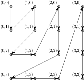
Figure 5. This figure depicts the order of the first 16 pairs in $\mathbb{N}_{0}^{2}$ with respect to the map $\mathcal{O}_{\mathbb{N}_{0}^{2}}$.

Figure 6. The first $49$ rectangles and their indices $\mathcal{O}_{\operatorname{\lhd\,}}$.

For a dyadic interval $I$, we write $I^{\ell}$ and $I^{r}$ for the dyadic intervals which are the left and right halves of $I$, respectively. In the following definition, we use the notation introduced in (4.5), so that for a collection $\mathscr{X}_{R}$ (respectively, $\mathscr{Y}_{R}$) of dyadic intervals, $X_{R}$ (respectively, $Y_{R}$) denotes its union.

Definition 4.7.

Let $\mathscr{A}=\mathscr{R}$ or $\mathscr{A}=\{R\in\mathscr{R}:R\operatorname{\unlhd\,}R_{0}\}$ for some $R_{0}\in\mathscr{R}$. We say that $\{\mathscr{B}_{R}:R\in\mathscr{A}\}$ satisfies the auxiliary condition (R1)–(R6) if the following properties hold true.

1. For each $R\in\mathscr{A}$, there are non-negative integers $\mu(R)$, $\nu(R)$ and non-empty sets $\mathscr{X}_{R}\subset\mathscr{D}_{\mu(R)}$ and $\mathscr{Y}_{R}\subset\mathscr{D}_{\nu(R)}$ such that $\mathscr{B}_{R}=\{K\times L:K\in\mathscr{X}_{R},\,L\in\mathscr{Y}_{R}\}$.

2. $\mu([0,1)\times[0,1))=\nu([0,1)\times[0,1))=0$ and $\mathscr{X}_{[0,1)\times[0,1)}=\mathscr{Y}_{[0,1)\times[0,1)}=\{[0,1)\}$.

3. For each $I\in\mathscr{D}\setminus\{[0,1)\}$ with $R=I\times[0,1)\in\mathscr{A}$

   $$X_{I\times[0,1)}=\begin{cases}\bigcup\{K^{\ell}:K\in\mathscr{D}_{\kappa(R)},\,K\subset X_{\widetilde{I}\times[0,1)}\}&\text{if}\ \ I=\widetilde{I}^{\ell},\\ \bigcup\{K^{r}:K\in\mathscr{D}_{\kappa(R)},\,K\subset X_{\widetilde{I}\times[0,1)}\}&\text{if}\ \ I=\widetilde{I}^{r},\end{cases}$$

   where $\kappa(R)=\max\{\mu(S):S\operatorname{\lhd\,}[0,|I|)\times[0,1)\}$;

4. If $R=I\times J\in\mathscr{A}$ with $|I|<|J|$, then

   $$\mu(R)>\max\{\mu(S):S\operatorname{\lhd\,}R\},$$

   $X_{R}=X_{I\times[0,1)}$, and $\mathscr{Y}_{R}=\mathscr{Y}_{I^{\prime}\times J}$, where $I^{\prime}\in\mathscr{D}$ is the unique dyadic interval such that $I^{\prime}\supset I$ and $|I^{\prime}|=|J|$.

5. For $J\in\mathscr{D}\setminus\{[0,1)\}$ with $R=[0,1)\times J\in\mathscr{A}$

   $$Y_{[0,1)\times J}=\begin{cases}\bigcup\{L^{\ell}:L\in\mathscr{D}_{\lambda(R)},\,L\subset Y_{[0,1)\times\widetilde{J}}\}&\text{if}\ \ J=\widetilde{J}^{\ell},\\ \bigcup\{L^{r}:L\in\mathscr{D}_{\lambda(R)},\,L\subset Y_{[0,1)\times\widetilde{J}}\}&\text{if}\ \ J=\widetilde{J}^{r},\end{cases}$$

   where $\lambda(R)=\max\{\nu(S):S\operatorname{\lhd\,}[0,1)\times[0,|J|)\}$.

6. If $R=I\times J\in\mathscr{A}\setminus\{[0,1)\times[0,1)\}$ with $|I|\geq|J|$, then

   $$\nu(R)>\max\{\nu(S):S\operatorname{\lhd\,}R\},$$

   $Y_{R}=Y_{[0,1)\times J}$, and $\mathscr{X}_{R}=\mathscr{X}_{I\times J^{\prime}}$, where $J^{\prime}\in\mathscr{D}$ is the unique dyadic interval such that $J^{\prime}\supset J$ and $|J^{\prime}|=2|I|$ if $I\neq[0,1)$, and $J^{\prime}=[0,1)$ if $I=[0,1)$.

Remark 4.8.

Let $\{\mathscr{B}_{R}:R\in\mathscr{R}\}$ be a collection such that each of the finite sub-collections $\{\mathscr{B}_{R}:R\operatorname{\unlhd\,}R_{0}\}$, $R_{0}\in\mathscr{R}$, satisfies the auxiliary condition (R1)–(R6). Then it is easy to see that $\{\mathscr{B}_{R}:R\in\mathscr{R}\}$ itself satisfies the auxiliary condition (R1)–(R6).

Lemma 4.9.

Let $\{\mathscr{B}_{R}:R\in\mathscr{R}\}$ satisfy the auxiliary condition (R1)–(R6). Then $\{\mathscr{B}_{R}:R\in\mathscr{R}\}$ satisfies the local product condition (P1)–(P4) with constants $C_{X}=C_{Y}=1$.

Proof.

The usual linear order $\prec$ on dyadic intervals is given by $I_{1}\prec I_{0}$ if and only if either $|I_{1}|>|I_{0}|$ or $|I_{1}|=|I_{0}|$ and $\min I_{1}<\min I_{0}$. The proof uses induction with respect to the linear orders $\prec$ and $\operatorname{\lhd\,}$.

Verification of (P1). For each $R\in\mathscr{R}$, $\mathscr{X}_{R}$ consists of pairwise disjoint intervals because $\mathscr{X}_{R}$ is contained in $\mathscr{D}_{\mu(R)}$. Similarly, $\mathscr{Y}_{R}\subset\mathscr{D}_{\nu(R)}$ and consists of pairwise disjoint intervals, and therefore the rectangles in $\mathscr{B}_{R}$ are pairwise disjoint.

Now suppose that $R_{0},R_{1}\in\mathscr{R}$ are distinct. By relabelling them if necessary, we may suppose that $R_{1}\operatorname{\lhd\,}R_{0}$, where $R_{0}=I_{0}\times J_{0}\neq[0,1)\times[0,1)$. To establish the disjointness of $\mathscr{B}_{R_{0}}$ and $\mathscr{B}_{R_{1}}$, we must show that either $\mathscr{X}_{R_{0}}$ and $\mathscr{X}_{R_{1}}$ are disjoint or $\mathscr{Y}_{R_{0}}$ and $\mathscr{Y}_{R_{1}}$ are disjoint. If $|I_{0}|<|J_{0}|$, then (R4) implies that $\mu(R_{0})>\mu(R_{1})$, so that $\mathscr{X}_{R_{0}}\cap\mathscr{X}_{R_{1}}\subset\mathscr{D}_{\mu(R_{0})}\cap\mathscr{D}_{\mu(R_{1})}=\emptyset$. Otherwise $|I_{0}|\geq|J_{0}|$, in which case a similar argument based on (R6) shows that $\mathscr{Y}_{R_{0}}\cap\mathscr{Y}_{R_{1}}=\emptyset$.

Verification of (P2). We begin by oberving that (R4) and (R6) imply that the sets $X_{R}$, $Y_{R}$, $X_{I}$, and $Y_{J}$ defined in (4.5)–(4.6) are given by

$$X_{R}=X_{I\times[0,1)}=X_{I}\qquad\text{and}\qquad Y_{R}=Y_{[0,1)\times J}=Y_{J},\qquad R=I\times J\in\mathscr{R}.$$ (4.27)

Since the order $\prec$ is linear, and the set $\mathscr{D}$ is countable and has a minimum element $[0,1)$ with respect to $\prec$, we may use induction on $I_{0}\in\mathscr{D}$ to prove the following two statements:

1. $X_{I_{0}\times[0,1)}\cap X_{I_{1}\times[0,1)}=\emptyset$ and $Y_{[0,1)\times I_{0}}\cap Y_{[0,1)\times I_{1}}=\emptyset$ for each $I_{1}\in\mathscr{D}$ with $I_{1}\prec I_{0}$ and $I_{0}\cap I_{1}=\emptyset$;

2. $X_{I_{0}\times[0,1)}\subset X_{I_{1}\times[0,1)}$ and $Y_{[0,1)\times I_{0}}\subset Y_{[0,1)\times I_{1}}$ for each $I_{1}\in\mathscr{D}$ with $I_{0}\subset I_{1}$.

The statements (a) and (b) above together with (4.27) imply (P2). The start of the induction is easy. Indeed, suppose that $I_{0}=[0,1)$. Then no $I_{1}$ satisfies $I_{1}\prec[0,1)$, so that (a) is vacuous, while (b) holds trivially because $I_{1}=[0,1)$ is the only dyadic interval which contains $[0,1)$.

Now let $I_{0}\in\mathscr{D}\setminus\{[0,1)\}$, and assume inductively that (a)–(b) have been established for each $I_{0}^{\prime}\prec I_{0}$ (that is, (a)–(b) hold whenever $I_{0}$ is replaced with $I_{0}^{\prime}$). We shall prove the statements concerning $X_{I_{0}\times[0,1)}$; the proofs for $Y_{[0,1)\times I_{0}}$ are similar, requiring only minor adjustments of the notation.

To verify (a), suppose that $I_{1}\in\mathscr{D}$ satisfies $I_{1}\prec I_{0}$ and $I_{0}\cap I_{1}=\emptyset$. Then either $I_{1}\cap\widetilde{I}_{0}=\emptyset$, or $I_{1}=(\widetilde{I}_{0})^{\ell}$ and $I_{0}=(\widetilde{I}_{0})^{r}$. (Note that because $I_{1}\prec I_{0}$, we cannot have $I_{1}=(\widetilde{I}_{0})^{r}$ and $I_{0}=(\widetilde{I}_{0})^{\ell}$.) In the first case, since $I_{1}\prec I_{0}$ and $\widetilde{I}_{0}\prec I_{0}$, the induction hypothesis implies that $X_{\widetilde{I}_{0}\times[0,1)}\cap X_{I_{1}\times[0,1)}=\emptyset$, from which the result follows because $X_{I_{0}\times[0,1)}\subset X_{\widetilde{I}_{0}\times[0,1)}$ by (R3).

In the second case, we observe that $\widetilde{I}_{0}=\widetilde{I}_{1}$ and $|I_{0}|=|I_{1}|$, so that $\kappa(I_{0}\times[0,1))=\kappa(I_{1}\times[0,1))$. This implies that $X_{I_{0}\times[0,1)}$ and $X_{I_{1}\times[0,1)}$ are disjoint because $X_{I_{0}\times[0,1)}$ is the disjoint union of the right halves of the intervals $K\in\mathscr{D}_{\kappa(I_{0}\times[0,1))}$ with $K\subset X_{\widetilde{I}_{0}\times[0,1)}$, while $X_{I_{1}\times[0,1)}$ is the disjoint union of the left halves of the same intervals.

Next, to prove (b), suppose that $I_{1}\in\mathscr{D}$ with $I_{0}\subset I_{1}$. The inclusion is obvious if $I_{0}=I_{1}$, so we may suppose that $I_{0}\subsetneq I_{1}$. Then we have $\widetilde{I}_{0}\subset I_{1}$, so the induction hypothesis implies that $X_{\widetilde{I}_{0}\times[0,1)}\subset X_{I_{1}\times[0,1)}$. Hence the statement follows from the fact that $X_{I_{0}\times[0,1)}\subset X_{\widetilde{I}_{0}\times[0,1)}$.

Verification of (P3). The proofs of (P3) and (P4) both rely on the following two identities:

$$|K\cap X_{I\times[0,1)}|=\frac{|K\cap X_{\widetilde{I}\times[0,1)}|}{2}\qquad\text{and}\qquad|L\cap Y_{[0,1)\times J}|=\frac{|L\cap Y_{[0,1)\times\widetilde{J}}|}{2},$$ (4.28)

valid for $I,J\in\mathscr{D}\setminus\{[0,1)\}$, $K\in\mathscr{D}^{\kappa(I\times[0,1))}$, and $L\in\mathscr{D}^{\lambda([0,1)\times J)}$.

We shall establish the first of these identities; again, the proof of the other requires only notational changes. For $I\in\mathscr{D}\setminus\{[0,1)\}$ and $K\in\mathscr{D}^{\kappa(I\times[0,1))}$, set $\mathscr{V}_{I}(K)=\{K_{0}\in\mathscr{D}_{\kappa(I\times[0,1))}:K_{0}\subset K\cap X_{\widetilde{I}\times[0,1)}\}$. We claim that

$$K\cap X_{\widetilde{I}\times[0,1)}=\bigcup\mathscr{V}_{I}(K)\quad\text{and}\quad K\cap X_{I\times[0,1)}=\begin{cases}\bigcup\{K_{0}^{\ell}:K_{0}\in\mathscr{V}_{I}(K)\}&\text{if}\ I=\widetilde{I}^{\ell}\\ \bigcup\{K_{0}^{r}:K_{0}\in\mathscr{V}_{I}(K)\}&\text{if}\ I=\widetilde{I}^{r}.\end{cases}$$ (4.29)

Indeed, the inclusion $\bigcup\mathscr{V}_{I}(K)\subset K\cap X_{\widetilde{I}\times[0,1)}$ is clear from the definition of $\mathscr{V}_{I}(K)$. Conversely, for each $x\in K\cap X_{\widetilde{I}\times[0,1)}$, there is a (necessarily unique) interval $K_{0}\in\mathscr{X}_{\widetilde{I}\times[0,1)}$ such that $x\in K_{0}$. We have $\mu(\widetilde{I}\times[0,1))\leq\kappa(I\times[0,1))$ because $\widetilde{I}\times[0,1)\operatorname{\lhd\,}[0,|I|)\times[0,1)$, so we can find $K_{1}\in\mathscr{D}_{\kappa(I\times[0,1))}$ such that $x\in K_{1}\subset K_{0}$. The sets $K_{1}$ and $K$ are not disjoint as they both contain $x$; combined with the fact that $|K_{1}|\leq|K|$, this shows that $K_{1}\subset K$. Moreover, we have $K_{1}\subset K_{0}\subset X_{\widetilde{I}\times[0,1)}$, so that $K_{1}\in\mathscr{V}_{I}(K)$, and hence $x\in K_{1}\subset\bigcup\mathscr{V}_{I}(K)$.

Moving on to the second part of (4.29), we obtain the inclusion $\supset$ directly from the definition of $\mathscr{V}_{I}(K)$ and (R3). Conversely, suppose that $x\in K\cap X_{I\times[0,1)}$, so that $x\in K$ and either $x\in K_{0}^{\ell}$ or $x\in K_{0}^{r}$ (depending on whether $I=(\widetilde{I})^{\ell}$ or $I=(\widetilde{I})^{r}$) for some $K_{0}\in\mathscr{D}_{\kappa(I\times[0,1))}$ with $K_{0}\subset X_{\widetilde{I}\times[0,1)}$. In both cases, we see that $K\cap K_{0}\neq\emptyset$ and $|K_{0}|\leq|K|$, so that $K_{0}\subset K$, and hence $K_{0}\in\mathscr{V}_{I}(K)$, from which the inclusion follows.

The first equation in (4.28) is immediate from (4.29) because $\mathscr{V}_{I}(K)$ consists of disjoint sets and $|K_{0}^{\ell}|=|K_{0}^{r}|=|K_{0}|/2$.

We can now easily establish (P3) with $C_{X}=C_{Y}=1$. By (4.27), we must show that

$$|X_{I\times[0,1)}|=|I|\qquad\text{and}\qquad|Y_{[0,1)\times I}|=|I|,\qquad I\in\mathscr{D}.$$ (4.30)

We do so by induction on $I$. The start of the induction, where $I=[0,1)$, follows immediately from the fact that $X_{[0,1)\times[0,1)}=Y_{[0,1)\times[0,1)}=[0,1)$ by (R2).

Now let $I\in\mathscr{D}\setminus\{[0,1)\}$, and assume inductively that the result is true for each $I^{\prime}\prec I$. Using (4.28) with $K=L=[0,1)$, we obtain that $|X_{I\times[0,1)}|=|X_{\widetilde{I}\times[0,1)}|/2=|\widetilde{I}|/2=|I|$ because $\widetilde{I}\prec I$ and likewise $|Y_{[0,1)\times I}|=|I|$.

Verification of (P4). We shall prove that, for each $R_{0}=I_{0}\times J_{0}$ and $R=I\times J$ in $\mathscr{R}$ with $R_{0}\subset R$,

$$\frac{|K\cap X_{I_{0}\times[0,1)}|}{|I_{0}|}=\frac{|K|}{|I|}\qquad\text{and}\qquad\frac{|L\cap Y_{[0,1)\times J_{0}}|}{|J_{0}|}=\frac{|L|}{|J|},\qquad K\in\mathscr{X}_{R},\,L\in\mathscr{Y}_{R}.$$ (4.31)

By (4.27) and (4.30), this will verify (P4) with $C_{X}=C_{Y}=1$.

The proof of (4.31) is by induction on $R_{0}$. The start of the induction is trivial because the only $R\in\mathscr{R}$ that contains $R_{0}=[0,1)\times[0,1)$ is $R_{0}$ itself.

Now let $R_{0}\in\mathscr{R}\setminus\{[0,1)\times[0,1)\}$, and assume inductively that (4.31) has been verified for each $R_{0}^{\prime}\operatorname{\lhd\,}R_{0}$. This time, we shall focus on the proof of the second identity in (4.31); the proof of the first identity is similar, but formally slightly easier due to the lack of symmetry between conditions (R4) and (R6): when $|I|=|J|$, we re-use an existing set as $\mathscr{X}_{R}$ and define a new set $\mathscr{Y}_{R}$.

Suppose that $R=I\times J\in\mathscr{R}$ with $R_{0}\subset R$, and let $L\in\mathscr{Y}_{R}$. If $J_{0}=J$, then $L\subset Y_{[0,1)\times J_{0}}$, and the identity is immediate. Hence we may suppose that $J_{0}\subsetneq J$. Moreover, we may suppose that $|I|\geq|J|$. Indeed, if not, then by (R4) $\mathscr{Y}_{R}=\mathscr{Y}_{I^{\prime}\times J}$, where $I^{\prime}\in\mathscr{D}$ satisfies $I^{\prime}\supset I$ and $|I^{\prime}|=|J|$, so that we may replace $I$ with $I^{\prime}$ to obtain that $|I|\geq|J|$.

Then we have $|J_{0}|<|J|=\min\{|I|,|J|\}$, so that $R\operatorname{\lhd\,}[0,1)\times[0,|J_{0}|)$, and hence $\lambda([0,1)\times J_{0})\geq\nu(R)$; thus $L\in\mathscr{Y}_{R}\subset\mathscr{D}_{\nu(R)}\subset\mathscr{D}^{\lambda([0,1)\times J_{0})}$, so that (4.28) shows that $|L\cap Y_{[0,1)\times J_{0}}|=|L\cap Y_{[0,1)\times\widetilde{J}_{0}}|/2$. Now $R_{0}^{\prime}=I_{0}\times\widetilde{J}_{0}$ satisfies $R_{0}^{\prime}\operatorname{\lhd\,}R_{0}$ and $R_{0}^{\prime}\subset R$, and therefore the induction hypothesis implies that $|L\cap Y_{[0,1)\times\widetilde{J}_{0}}|/|\widetilde{J}_{0}|=|L|/|J|$. Hence the conclusion follows because $|\widetilde{J}_{0}|=2|J_{0}|$.∎

Having obtained Theorem 4.3 and Lemma 4.9, we are finally prepared to prove Theorem 3.1.

5. Proof of Theorem 3.1

Here, we prove that the identity operator on $H^{p}(H^{q})$ factors through any operator $T:H^{p}(H^{q})\to H^{p}(H^{q})$ having large diagonal with respect to the bi-parameter Haar system (see Theorem 3.1). The basic pattern of our argument below is the following: we carefully construct $\{\mathscr{B}_{R}:R\in\mathscr{R}\}$ satisfying the auxiliary condition (R1)–(R6) (see Section 4). Moreover, these collections are chosen in such a way that we are able to find signs $\varepsilon_{Q}\in\{\pm 1\}$, $Q\in\bigcup_{R\in\mathscr{R}}\mathscr{B}_{R}$, for which the block basis $b_{R}^{(\varepsilon)}=\sum_{Q\in\mathscr{B}_{R}}\varepsilon_{Q}h_{Q}$, $R\in\mathscr{R}$ has the following properties: $|\langle Tb_{R_{1}}^{(\varepsilon)},b_{R_{2}}^{(\varepsilon)}\rangle|$ is small in the precise sense of (5.6a) below whenever $R_{1},R_{2}\in\mathscr{R}$ are distinct, and

$$|\langle Tb_{R}^{(\varepsilon)},b_{R}^{(\varepsilon)}\rangle|\geq\delta\|b_{R}^{(\varepsilon)}\|_{2}^{2},\qquad R\in\mathscr{R}.$$

Thereafter we apply the two main results of the preceding section, Theorem 4.3 and Lemma 4.9, and finally we construct a factorization of the identity operator through $T$.

Proof of Theorem 3.1.

Let $1\leq p,q<\infty$ and $\delta>0$, and let $T:H^{p}(H^{q})\to H^{p}(H^{q})$ be an operator such that

$$|\langle Th_{R},h_{R}\rangle|\geq\delta|R|,\qquad R\in\mathscr{R}.$$ (5.1)

We define $\gamma=(\gamma_{R}:R\in\mathscr{R})$ by

$$\gamma_{R}=\frac{\overline{\langle Th_{R},h_{R}\rangle}}{|\langle Th_{R},h_{R}\rangle|},\qquad R\in\mathscr{R}.$$

Recall that in (4.2) we defined the Haar multiplier $M_{\gamma}$ which satisfies $\|M_{\gamma}\|=1$, and $\langle(TM_{\gamma})h_{R},h_{R}\rangle\geq\delta|R|$. Thereby, replacing $T$ with $TM_{\gamma}$, it suffices to consider the special case where

$$\langle Th_{R},h_{R}\rangle\geq\delta|R|,\qquad R\in\mathscr{R}.$$ (5.2)

Overview. Let $0<\eta\leq 1$. The main part of the proof consists of choosing collections of dyadic rectangles $\mathscr{B}_{R}$, $R\in\mathscr{R}$ and suitable signs $\varepsilon=(\varepsilon_{Q})$ such that $b_{R}^{(\varepsilon)}=\sum_{Q\in\mathscr{B}_{R}}\varepsilon_{Q}h_{Q}$ satisfies the following:

• The closed linear span of $\{b_{R}^{(\varepsilon)}:R\in\mathscr{R}\}$ is complemented and isomorphic to $H^{p}(H^{q})$.

• There is an operator $U:H^{p}(H^{q})\to H^{p}(H^{q})$ given by

  $$U(f)=\sum_{R\in\mathscr{R}}\frac{\langle f,b_{R}^{(\varepsilon)}\rangle}{\langle Tb_{R}^{(\varepsilon)},b_{R}^{(\varepsilon)}\rangle}b_{R}^{(\varepsilon)}.$$

• For every finite linear combination $g=\sum_{R\in\mathscr{R}}\lambda_{R}b_{R}^{(\varepsilon)}$ we have

  $$\|UTg-g\|_{H^{p}(H^{q})}\leq\frac{\eta}{2}\|g\|_{H^{p}(H^{q})}.$$

Preparation. Given $R=I\times J\in\mathscr{R}$ we write

$$Th_{R}=\alpha_{R}h_{R}+r_{R},$$ (5.3a)

where

$$\alpha_{R}=\frac{\langle Th_{R},h_{R}\rangle}{|R|}\qquad\text{and}\qquad r_{R}=\sum_{S\neq R}\frac{\langle Th_{R},h_{S}\rangle}{|S|}h_{S}.$$ (5.3b)

We note the estimates

$$\delta\leq\alpha_{R}\leq\|T\|\qquad\text{and}\qquad\|r_{R}\|_{H^{p}(H^{q})}\leq 2\|T\||I|^{1/p}|J|^{1/q}.$$ (5.4)

Inductive construction of $b_{R}^{(\varepsilon)}$. We will now inductively define the block basis $\{b_{R}^{(\varepsilon)}\,:\,R\in\mathscr{R}\}$. For fixed $R\in\mathscr{R}$, the block basis element $b_{R}^{(\varepsilon)}$ is determined by a collection of dyadic rectangles $\mathscr{B}_{R}\subset\mathscr{R}$ and a suitable choice of signs $\varepsilon=(\varepsilon_{Q})$ and is of the following form:

$$b_{R}^{(\varepsilon)}=\sum_{Q\in\mathscr{B}_{R}}\varepsilon_{Q}h_{Q}.$$ (5.5)

From now on, we systematically use the following rule: whenever $\mathcal{O}_{\operatorname{\lhd\,}}(R)=i$ we set

$$\mathscr{B}_{i}=\mathscr{B}_{R},\qquad b_{i}^{(\varepsilon)}=b_{R}^{(\varepsilon)},\qquad h_{i}=h_{R}.$$

We will construct collections $\{\mathscr{B}_{i}:i\in\mathbb{N}_{0}\}$ satisfying the auxiliary condition (R1)–(R6) and choose signs $\varepsilon=(\varepsilon_{Q})$ such that

$$\sum_{j=0}^{i-1}|\langle Tb_{j}^{(\varepsilon)},b_{i}^{(\varepsilon)}\rangle|+|\langle b_{i}^{(\varepsilon)},T^{*}b_{j}^{(\varepsilon)}\rangle| \leq\eta\delta 4^{-i-2},\qquad i\in\mathbb{N},$$ (5.6a)

$$|\langle Tb_{i}^{(\varepsilon)},b_{i}^{(\varepsilon)}\rangle| \geq\delta\|b_{i}^{(\varepsilon)}\|_{2}^{2},\qquad i\in\mathbb{N}_{0}.$$ (5.6b)

The induction begins by putting

$$\mathscr{B}_{0}=\{[0,1)\times[0,1)\}\qquad\text{and}\qquad b_{0}^{(\varepsilon)}=h_{[0,1)\times[0,1)}.$$ (5.7)

Consequently, $\mathscr{X}_{[0,1)\times[0,1)}=\mathscr{Y}_{[0,1)\times[0,1)}=\{[0,1)\}$ and $\mu([0,1)\times[0,1))=0$, $\nu([0,1)\times[0,1))=0$. Obviously, $\{\mathscr{B}_{0}\}$ satisfies (R1)–(R6).

Let $i_{0}\in\mathbb{N}$. At this stage we assume that

• $\{\mathscr{B}_{j}:0\leq j\leq i_{0}-1\}$ satisfies the auxiliary condition (R1)–(R6).

• the block basis $\{b_{j}^{(\varepsilon)}:0\leq j\leq i_{0}-1\}$ given by (5.5) satisfies (5.6) (for $0\leq i\leq i_{0}-1$).

Now, we turn to the construction of $\mathscr{B}_{i_{0}}$ and $\varepsilon_{Q}$, where $Q\in\mathscr{B}_{i_{0}}$. In the first step we will find $\mathscr{B}_{i_{0}}$ in (5.20), and only then we will choose the signs $\varepsilon_{Q}$, $Q\in\mathscr{B}_{i_{0}}$ in (5.23). The collection $\mathscr{B}_{i_{0}}$ and the signs $\varepsilon_{Q}$, $Q\in\mathscr{B}_{i_{0}}$ then determine $b_{i_{0}}^{(\varepsilon)}$.

Construction of $\mathscr{B}_{i_{0}}$. Let $I_{0}\times J_{0}\in\mathscr{R}$ be such that $\mathcal{O}_{\operatorname{\lhd\,}}(I_{0}\times J_{0})=i_{0}$. We distinguish between the four cases

$$|I_{0}|<|J_{0}|,J_{0}=[0,1),\qquad|I_{0}|<|J_{0}|,J_{0}\neq[0,1),$$

and

$$|I_{0}|\geq|J_{0}|,I_{0}=[0,1),\qquad|I_{0}|\geq|J_{0}|,I_{0}\neq[0,1).$$

Case 1: $|I_{0}|<|J_{0}|$. Here, we will construct the collection $\mathscr{B}_{I_{0}\times J_{0}}$, for which the index rectangle $I_{0}\times J_{0}$ is “below the diagonal”.

First, we define

$$\nu(I_{0}\times J_{0})=\nu(I_{0}^{\prime}\times J_{0})\qquad\text{and}\qquad\mathscr{Y}_{I_{0}\times J_{0}}=\mathscr{Y}_{I_{0}^{\prime}\times J_{0}},$$ (5.8)

where $I_{0}^{\prime}\in\mathscr{D}$ is the unique interval such that $I_{0}^{\prime}\supset I_{0}$ and $|I_{0}^{\prime}|=|J_{0}|$. We remark that $\mu(I_{0}\times J_{0})$ will be defined at the end of the proof in (5.21a).

Case 1.a: $J_{0}=[0,1)$. Here, we know that $I_{0}\neq[0,1)$. Recall that $\widetilde{I}_{0}$ denotes the dyadic predecessor of $I_{0}$, and note that $\mathscr{B}_{\widetilde{I}_{0}\times[0,1)}$ has already been defined. The collections indexed by the black rectangles have already been constructed. Here, we determine the collections for the gray rectangles. The white ones will be treated later.

Note that $[0,|I_{0}|)\times[0,1)\operatorname{\unlhd\,}I_{0}\times[0,1)$, and define the integer $\kappa(I_{0}\times[0,1))$ by

$$\kappa(I_{0}\times[0,1))=\max\{\mu(Q):Q\operatorname{\lhd\,}[0,|I_{0}|)\times[0,1)\}.$$

Recall that for a dyadic interval $K_{0}$ we denote its left half by $K_{0}^{\ell}$ and its right half by $K_{0}^{r}$. Following the basic construction of Gamlen-Gaudet [5], we proceed as follows. The set $X_{\widetilde{I_{0}}\times[0,1)}$ has already been defined in a previous step of the construction. Now we put

$$X_{I_{0}\times[0,1)}=\begin{cases}\bigcup\{K_{0}^{\ell}:K_{0}\in\mathscr{D}_{\kappa(I_{0}\times[0,1))},\,K_{0}\subset X_{\widetilde{I_{0}}\times[0,1)}\}&\text{if}\ \ I_{0}=\widetilde{I_{0}}^{\ell},\\ \bigcup\{K_{0}^{r}:K_{0}\in\mathscr{D}_{\kappa(I_{0}\times[0,1))},\,K_{0}\subset X_{\widetilde{I_{0}}\times[0,1)}\}&\text{if}\ \ I_{0}=\widetilde{I_{0}}^{r}.\end{cases}$$

To finish the construction in Case 1.a, we define the family of high frequency covers of the set $X_{I_{0}\times[0,1)}\times[0,1)$ by putting

$$\mathscr{F}_{m}=\{K\times[0,1)\in\mathscr{R}\,:\,K\in\mathscr{D}_{m},\,K\subset X_{I_{0}\times[0,1)}\},$$ (5.9)

for all $m>\kappa(I_{0}\times[0,1))$, see Figure 7, and observe that

$$\bigcup\mathscr{F}_{m}=X_{I_{0}\times[0,1)}\times[0,1).$$ (5.10)

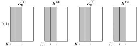
Figure 7. The above figure depicts an instance of $\mathscr{F}_{m}$ in Case 1.a. $K_{0}^{(k)}$ is a dyadic interval such that $K_{0}^{(k)}\times[0,1)\in\mathscr{B}_{\widetilde{I}_{0}\times[0,1)}$, and $K$ is a dyadic interval such that $K\times[0,1)\in\mathscr{F}_{m}$.

Case 1.b: $J_{0}\neq[0,1)$. The collections indexed by the black rectangles have already been constructed. Here, we determine the collections for the gray rectangles. The white ones will be treated later.

By our induction hypothesis, $\{\mathscr{B}_{I\times J}:\mathcal{O}_{\operatorname{\lhd\,}}(I\times J)\leq i_{0}-1\}$ satisfies (R1)–(R6). Note that the set $X_{I_{0}\times[0,1)}$ is already defined. To conclude the construction in Case 1.b, we define the high frequency covers of $X_{I_{0}\times[0,1)}\times Y_{I_{0}\times J_{0}}$ by

$$\mathscr{F}_{m}=\{K\times L_{0}\in\mathscr{R}\,:\,K\in\mathscr{D}_{m},\,K\subset X_{I_{0}\times[0,1)},\ L_{0}\in\mathscr{Y}_{I_{0}\times J_{0}}\},$$ (5.11)

for $m>\mu({I_{0}\times\widetilde{J}_{0}})$.

Case 2: $|I_{0}|\geq|J_{0}|$. In this case, we will construct the collection $\mathscr{B}_{I_{0}\times J_{0}}$, for which the index rectangle $I_{0}\times J_{0}$ is “on or above the diagonal”.

First, we set

$$\mu(I_{0}\times J_{0})=\mu(I_{0}\times J_{0}^{\prime})\qquad\text{and}\qquad\mathscr{X}_{I_{0}\times J_{0}}=\mathscr{X}_{I_{0}\times J_{0}^{\prime}},$$ (5.12)

where $J_{0}^{\prime}\in\mathscr{D}$ is the unique dyadic interval such that $J_{0}^{\prime}\supset J_{0}$ and $|J_{0}^{\prime}|=2|I|$ if $I\neq[0,1)$, and $J_{0}^{\prime}=[0,1)$ if $I=[0,1)$. We remark that $\nu(I_{0}\times J_{0})$ will be defined at the end of the proof in (5.21b).

Case 2.a: $I_{0}=[0,1)$. Note that $J_{0}\neq[0,1)$ and $\mathscr{B}_{[0,1)\times\widetilde{J}_{0}}$ has already been constructed. The collections indexed by the black rectangles have already been constructed. Here, we determine the collections for the gray rectangles. The white ones will be treated later.

Note that $[0,1)\times[0,|J_{0}|)\operatorname{\unlhd\,}[0,1)\times J_{0}$. Define $\lambda([0,1)\times J_{0})$ to be

$$\lambda([0,1)\times J_{0})=\max\{\nu(Q):Q\operatorname{\lhd\,}[0,1)\times[0,|J_{0}|)\}.$$ (5.13)

Recall that for a dyadic interval $L_{0}$ we denote its left (=lower) half by $L_{0}^{\ell}$ and its right (=upper) half by $L_{0}^{r}$. The set $Y_{[0,1)\times\widetilde{J}_{0}}$ has already been defined. Now, put

$$Y_{[0,1)\times J_{0}}=\begin{cases}\bigcup\{L_{0}^{\ell}:L_{0}\in\mathscr{D}_{\lambda([0,1)\times J_{0})},\,L_{0}\subset Y_{[0,1)\times\widetilde{J}_{0}}\}&\text{if}\ \ J_{0}=\widetilde{J}_{0}^{\ell},\\ \bigcup\{L_{0}^{r}:L_{0}\in\mathscr{D}_{\lambda([0,1)\times J_{0})},\,L_{0}\subset Y_{[0,1)\times\widetilde{J}_{0}}\}&\text{if}\ \ J_{0}=\widetilde{J}_{0}^{r}.\end{cases}$$

We define the family of high frequency covers of the set $[0,1)\times Y_{[0,1)\times J_{0}}$ by

$$\mathscr{F}_{m}=\{[0,1)\times L\in\mathscr{R}\,:\,L\in\mathscr{D}_{m},\,L\subset Y_{[0,1)\times J_{0}}\},$$ (5.14)

for all $m>\lambda([0,1)\times J_{0})$, see Figure 8, and observe that

$$\bigcup\mathscr{F}_{m}=[0,1)\times Y_{[0,1)\times J_{0}}.$$ (5.15)

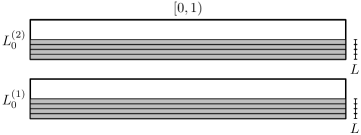
Figure 8. The above figure depicts an instance of $\mathscr{F}_{m}$ in Case 2.a. $L_{0}^{(k)}$ is a dyadic interval such that $[0,1)\times L_{0}^{(k)}\in\mathscr{B}_{[0,1)\times\widetilde{J}_{0}}$, and $L$ is a dyadic interval such that $[0,1)\times L\in\mathscr{F}_{m}$.

Case 2.b: $I_{0}\neq[0,1)$. The collections indexed by the black rectangles have already been constructed. Here, we determine the collections for the gray rectangles.

By our induction hypothesis, $\{\mathscr{B}_{I\times J}:\mathcal{O}_{\operatorname{\lhd\,}}(I\times J)\leq i_{0}-1\}$ satisfies (R1)–(R6). At this stage of the proof, the set $Y_{[0,1)\times J_{0}}$ has already been constructed. Now, we define the high frequency covers of $X_{I_{0}\times J_{0}}\times Y_{[0,1)\times J_{0}}$ by putting

$$\mathscr{F}_{m}=\{K_{0}\times L\,:\,K_{0}\in\mathscr{X}_{I_{0}\times J_{0}},\,L\in\mathscr{D}_{m},\,L\subset Y_{[0,1)\times J_{0}}\},$$ (5.16)

whenever $m>\nu(\widetilde{I}_{0}\times J_{0})$, see Figure 9.

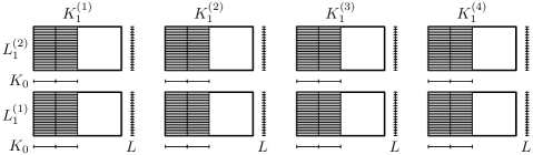
Figure 9. The above figure depicts an instance of $\mathscr{F}_{m}$ in Case 2.b. We have $K_{1}^{(k)}\in\mathscr{X}_{\widetilde{I}_{0}\times J_{0}}$, $L_{1}^{(\ell)}\in\mathscr{Y}_{\widetilde{I}_{0}\times J_{0}}$, and the dyadic interval $K_{0}$ is in $\mathscr{X}_{I_{0}\times J_{0}}$. $\mathscr{F}_{m}$ is the collection of all the small gray rectangles. We obtain $\mathscr{F}_{m}$ by leaving intact the intervals of the $x$-coordinate ($K_{0}\in\mathscr{X}_{I_{0}\times J_{0}}$) and using a high frequency cover – comprised of the intervals $L$ – of the intervals $L_{1}^{(\ell)}\in\mathscr{Y}_{\widetilde{I}_{0}\times J_{0}}$. The intervals $L_{1}^{(\ell)}\in\mathscr{Y}_{\widetilde{I}_{0}\times J_{0}}$ in this Figure are covering the exact same set as the intervals denoted by $L$ in Figure 8, i.e. they cover $Y_{[0,1)\times J_{0}}$.

In each of the above cases (5.9), (5.11), (5.14), and (5.16) we define the following functions. Firstly, let

$$f_{m}=\sum_{Q\in\mathscr{F}_{m}}h_{Q},$$ (5.17a)

and secondly for any choice of signs $$\varepsilon_{Q}\in\{-1,+1\} Q\in\mathscr{F}_{m}$$, put

$$f_{m}^{(\varepsilon)}=\sum_{Q\in\mathscr{F}_{m}}\varepsilon_{Q}h_{Q}.$$ (5.17b)

Now, we specify the value of $m$. To this end, put

$$k_{i_{0}}=\max\{\mu(R),\nu(R):R\in\mathscr{R},\ \mathcal{O}_{\operatorname{\lhd\,}}(R)\leq i_{0}-1\},$$ (5.18)

and note that each $\mathscr{F}_{m}$, $m>k_{i_{0}}$ can be written as the product of two sets of intervals, i.e.

$$\mathscr{F}_{m}=\{K\times L:K\in\mathscr{X}_{m},\ L\in\mathscr{Y}_{m}\},\qquad m>k_{i_{0}},$$

where the collections $\mathscr{X}_{m}$ and $\mathscr{Y}_{m}$, $m>k_{i_{0}}$, satisfy the following:

• $\mathscr{X}_{m}$ and $\mathscr{Y}_{m}$ are each a non-empty, finite collection of pairwise disjoint dyadic intervals of equal length, whenever $m>k_{i_{0}}$;

• $\mathscr{X}_{m}\cap\mathscr{X}_{n}=\emptyset$ or $\mathscr{Y}_{m}\cap\mathscr{Y}_{n}=\emptyset$ whenever $m,n>k_{i_{0}}$ are distinct;

• the union of the sets in $\mathscr{X}_{m}$ is independent of $m>k_{i_{0}}$, and the union of the sets in $\mathscr{Y}_{m}$ is independent of $m>k_{i_{0}}$.

Thus, by Lemma 4.1, we have that

• for each $g\in H^{p}(H^{q})^{*}$, $\sup_{\gamma\in\Gamma}|\langle M_{\gamma}f_{m},g\rangle|\to 0$ as $m\to\infty;$

• for each $g\in H^{p}(H^{q})$, $\sup_{\gamma\in\Gamma}|\langle M_{\gamma}g,f_{m}\rangle|\to 0$ as $m\to\infty$;

where we recall that $\Gamma$ denotes the unit ball of $\ell^{\infty}(\mathscr{R})$, and that $\gamma=(\gamma_{R}:R\in\mathscr{R})\in\Gamma$ defines the operator $M_{\gamma}$ (see (4.2)). Hence, we can find an integer $m_{i_{0}}>k_{i_{0}}$ such that

$$\sum_{j=0}^{i_{0}-1}|\langle Tb_{j}^{(\varepsilon)},f_{m_{i_{0}}}^{(\varepsilon)}\rangle|+|\langle f_{m_{i_{0}}}^{(\varepsilon)},T^{*}b_{j}^{(\varepsilon)}\rangle|\leq\eta\delta 4^{-i_{0}-2},$$ (5.19)

for all choices of signs $\varepsilon_{K\times L}$, $K\times L\in\mathscr{F}_{m_{i_{0}}}$. Now, we put

$$\mathscr{B}_{I_{0}\times J_{0}}=\mathscr{B}_{i_{0}}=\mathscr{F}_{m_{i_{0}}}.$$ (5.20)

If $$I_{0}\times J_{0} |I_{0}|<|J_{0}|$$ is a “Case 1” rectangle, i.e. , then

$$\mu(I_{0}\times J_{0})=m_{i_{0}}\quad\text{and}\quad\mathscr{X}_{I_{0}\times J_{0}}=\{I\in\mathscr{D}_{m_{i_{0}}}:I\times J\in\mathscr{B}_{I_{0}\times J_{0}}\},$$ (5.21a)

and if $$I_{0}\times J_{0} |I_{0}|\geq|J_{0}|$$ is a “Case 2” rectangle, i.e. , then

$$\nu(I_{0}\times J_{0})=m_{i_{0}}\quad\text{and}\quad\mathscr{Y}_{I_{0}\times J_{0}}=\{J\in\mathscr{D}_{m_{i_{0}}}:I\times J\in\mathscr{B}_{I_{0}\times J_{0}}\}.$$ (5.21b)

Thereby, we have completed the construction of $\mathscr{B}_{I_{0}\times J_{0}}=\mathscr{B}_{i_{0}}$.

Reviewing the four cases Case 1.a, Case 1.b, Case 2.a, and Case 2.b of the construction we see that $\{\mathscr{B}_{i}:i\leq i_{0}\}$ satisfies (R1)–(R6).

Selecting the signs $\varepsilon$. Let $\varepsilon_{Q}\in\{\pm 1\}$, $Q\in\mathscr{B}_{i_{0}}$ be fixed. We obtain from (5.3) and (5.17)

$$\langle Tf_{m_{i_{0}}}^{(\varepsilon)},f_{m_{i_{0}}}^{(\varepsilon)}\rangle=\sum_{Q\in\mathscr{B}_{i_{0}}}\alpha_{Q}|Q|+\langle f_{m_{i_{0}}}^{(\varepsilon)},s_{m_{i_{0}}}^{(\varepsilon)}\rangle,$$

where

$$s_{m_{i_{0}}}^{(\varepsilon)}=\sum_{Q\in\mathscr{B}_{i_{0}}}\varepsilon_{Q}r_{Q}.$$

By (5.3) we have $\langle h_{Q},r_{Q}\rangle=0$, $Q\in\mathscr{R}$, and consequently

$$\langle f_{m_{i_{0}}}^{(\varepsilon)},s_{m_{i_{0}}}^{(\varepsilon)}\rangle=\sum\varepsilon_{Q_{0}}\varepsilon_{Q_{1}}\langle h_{Q_{0}},r_{Q_{1}}\rangle,$$ (5.22)

where the sum is taken over all $Q_{0},Q_{1}\in\mathscr{B}_{i_{0}}$ with $Q_{0}\neq Q_{1}$. Let $\operatorname{\mathbb{E}}_{\varepsilon}$ denote the average over all possible choices of signs $\varepsilon_{Q}$, $Q\in\mathscr{B}_{i_{0}}$. Taking expectations we obtain from (5.22) that

$$\operatorname{\mathbb{E}}_{\varepsilon}\langle f_{m_{i_{0}}}^{(\varepsilon)},s_{m_{i_{0}}}^{(\varepsilon)}\rangle=0.$$

This gives us

$$\operatorname{\mathbb{E}}_{\varepsilon}\langle Tf_{m_{i_{0}}}^{(\varepsilon)},f_{m_{i_{0}}}^{(\varepsilon)}\rangle=\sum_{Q\in\mathscr{B}_{i_{0}}}\alpha_{Q}|Q|.$$

Hence, in view of (5.4), there exists at least one $\varepsilon$ such that

$$|\langle Tf_{m_{i_{0}}}^{(\varepsilon)},f_{m_{i_{0}}}^{(\varepsilon)}\rangle|\geq\sum_{Q\in\mathscr{B}_{i_{0}}}\alpha_{Q}|Q|\geq\delta\|f_{m_{i_{0}}}^{(\varepsilon)}\|_{2}^{2}.$$ (5.23)

We complete the inductive construction by choosing $\varepsilon$ according to (5.23) and define

$$b_{I_{0}\times J_{0}}^{(\varepsilon)}=b_{i_{0}}^{(\varepsilon)}=f_{m_{i_{0}}}^{(\varepsilon)}.$$ (5.24)

Hence, (5.6b) holds for $i=i_{0}$, while (5.19) ensures that (5.6a) holds for $i=i_{0}$.

Essential properties of our inductive construction. Since each of the finite collections $\{\mathscr{B}_{i}:i\leq i_{0}\}$, $i_{0}\in\mathbb{N}_{0}$, satisfies (R1)–(R6), Remark 4.8 asserts that the infinite collection $\{\mathscr{B}_{i}:i\in\mathbb{N}_{0}\}$ satisfies (R1)–(R6), and hence, by Lemma 4.9, it satisfies the local product condition (P1)–(P4) with constants $C_{X}=C_{Y}=1$.

For $1\leq u,v<\infty$ and $I\times J\in\mathscr{R}$, Lemma 4.1(i)–(ii) together with (4.7) and (P3) gives us the following mixed-norm estimates for $b_{I\times J}^{(\varepsilon)}$:

$$\|b_{I\times J}^{(\varepsilon)}\|_{H^{u}(H^{v})} =|I|^{1/u}|J|^{1/v}=\|h_{I\times J}\|_{H^{u}(H^{v})},$$ (5.25a)

$$\|b_{I\times J}^{(\varepsilon)}\|_{H^{u}(H^{v})^{*}} =|I|^{1-1/u}|J|^{1-1/v}=\|h_{I\times J}\|_{H^{u}(H^{v})^{*}}.$$ (5.25b)

The estimates (5.6a) and (5.6b) show that the block basis $\{b_{i}^{(\varepsilon)}\}$ almost-diagonalizes $T$ in the following precise sense:

$$|\langle Tb_{i}^{(\varepsilon)},b_{i}^{(\varepsilon)}\rangle| \geq\delta\|b_{i}^{(\varepsilon)}\|_{2}^{2},\qquad i\in\mathbb{N}_{0},$$ (5.26)

$$\sum_{j=0}^{i-1}|\langle Tb_{j}^{(\varepsilon)},b_{i}^{(\varepsilon)}\rangle|+|\langle Tb_{i}^{(\varepsilon)},b_{j}^{(\varepsilon)}\rangle| \leq\eta\delta 4^{-i-2},\qquad i\in\mathbb{N}.$$ (5.27)

Putting it together. The basic model of argument presented below can be traced to the seminal paper of Alspach, Enflo, and Odell [1]. Since $\{\mathscr{B}_{I\times J}\}$ satisfies the local product condition (P1)–(P4) with constants $C_{X}=C_{Y}=1$, we obtain from Theorem 4.3 the following. First, let $Y=\overline{\operatorname{span}}\{b_{i}^{(\varepsilon)}\,:\,i\in\mathbb{N}_{0}\}\subset H^{p}(H^{q})$ and let $B_{\varepsilon}:H^{p}(H^{q})\to Y$ denote the unique linear extension of $B_{\varepsilon}h_{i}=b_{i}^{(\varepsilon)}$, $i\in\mathbb{N}_{0}$, then by Theorem 4.3

$$\vbox{\lx@xy@svg{\hbox{\raise 0.0pt\hbox{\kern 18.77304pt\hbox{\ignorespaces\ignorespaces\ignorespaces\hbox{\vtop{\kern 0.0pt\offinterlineskip\halign{\entry@#!@&&\entry@@#!@\cr&\\&\crcr}}}\ignorespaces{\hbox{\kern-18.77304pt\raise 0.0pt\hbox{\hbox{\kern 0.0pt\raise 0.0pt\hbox{\hbox{\kern 3.0pt\raise 0.0pt\hbox{$\textstyle{H^{p}(H^{q})\ignorespaces\ignorespaces\ignorespaces\ignorespaces\ignorespaces\ignorespaces\ignorespaces\ignorespaces}$}}}}}}}\ignorespaces\ignorespaces\ignorespaces\ignorespaces{}{\hbox{\lx@xy@droprule}}\ignorespaces\ignorespaces\ignorespaces{\hbox{\kern 19.17766pt\raise 6.74722pt\hbox{{}\hbox{\kern 0.0pt\raise 0.0pt\hbox{\hbox{\kern 3.0pt\hbox{\hbox{\kern 0.0pt\raise-1.03612pt\hbox{$\scriptstyle{I_{H^{p}(H^{q})}}$}}}\kern 3.0pt}}}}}}\ignorespaces{\hbox{\kern 42.77304pt\raise 0.0pt\hbox{\hbox{\kern 0.0pt\raise 0.0pt\hbox{\lx@xy@tip{1}\lx@xy@tip{-1}}}}}}{\hbox{\lx@xy@droprule}}{\hbox{\lx@xy@droprule}}\ignorespaces\ignorespaces\ignorespaces\ignorespaces{}{\hbox{\lx@xy@droprule}}\ignorespaces\ignorespaces\ignorespaces{\hbox{\kern-13.52602pt\raise-19.34303pt\hbox{{}\hbox{\kern 0.0pt\raise 0.0pt\hbox{\hbox{\kern 3.0pt\hbox{\hbox{\kern 0.0pt\raise-1.9611pt\hbox{$\scriptstyle{B_{\varepsilon}}$}}}\kern 3.0pt}}}}}}\ignorespaces{\hbox{\kern 0.0pt\raise-28.85277pt\hbox{\hbox{\kern 0.0pt\raise 0.0pt\hbox{\lx@xy@tip{1}\lx@xy@tip{-1}}}}}}{\hbox{\lx@xy@droprule}}{\hbox{\lx@xy@droprule}}{\hbox{\kern 42.77304pt\raise 0.0pt\hbox{\hbox{\kern 0.0pt\raise 0.0pt\hbox{\hbox{\kern 3.0pt\raise 0.0pt\hbox{$\textstyle{H^{p}(H^{q})}$}}}}}}}{\hbox{\kern-7.01389pt\raise-38.68608pt\hbox{\hbox{\kern 0.0pt\raise 0.0pt\hbox{\hbox{\kern 3.0pt\raise 0.0pt\hbox{$\textstyle{Y\ignorespaces\ignorespaces\ignorespaces\ignorespaces}$}}}}}}}\ignorespaces\ignorespaces\ignorespaces\ignorespaces{}{\hbox{\lx@xy@droprule}}\ignorespaces\ignorespaces\ignorespaces{\hbox{\kern 24.35431pt\raise-44.76108pt\hbox{{}\hbox{\kern 0.0pt\raise 0.0pt\hbox{\hbox{\kern 3.0pt\hbox{\hbox{\kern 0.0pt\raise-1.70833pt\hbox{$\scriptstyle{I_{Y}}$}}}\kern 3.0pt}}}}}}\ignorespaces{\hbox{\kern 54.5322pt\raise-38.68608pt\hbox{\hbox{\kern 0.0pt\raise 0.0pt\hbox{\lx@xy@tip{1}\lx@xy@tip{-1}}}}}}{\hbox{\lx@xy@droprule}}{\hbox{\lx@xy@droprule}}{\hbox{\kern 54.5322pt\raise-38.68608pt\hbox{\hbox{\kern 0.0pt\raise 0.0pt\hbox{\hbox{\kern 3.0pt\raise 0.0pt\hbox{$\textstyle{Y\ignorespaces\ignorespaces\ignorespaces\ignorespaces}$}}}}}}}\ignorespaces\ignorespaces\ignorespaces\ignorespaces{}{\hbox{\lx@xy@droprule}}\ignorespaces\ignorespaces\ignorespaces{\hbox{\kern 61.54608pt\raise-19.34305pt\hbox{{}\hbox{\kern 0.0pt\raise 0.0pt\hbox{\hbox{\kern 3.0pt\hbox{\hbox{\kern 0.0pt\raise-1.75pt\hbox{$\scriptstyle{A_{\varepsilon}|Y}$}}}\kern 3.0pt}}}}}}\ignorespaces{\hbox{\kern 61.54608pt\raise-5.5pt\hbox{\hbox{\kern 0.0pt\raise 0.0pt\hbox{\lx@xy@tip{1}\lx@xy@tip{-1}}}}}}{\hbox{\lx@xy@droprule}}{\hbox{\lx@xy@droprule}}\ignorespaces}}}}\ignorespaces}\qquad\|B_{\varepsilon}\|=\|A_{\varepsilon}\|=1, \textstyle{H^{p}(H^{q})\ignorespaces\ignorespaces\ignorespaces\ignorespaces\ignorespaces\ignorespaces\ignorespaces\ignorespaces} \scriptstyle{I_{H^{p}(H^{q})}} \scriptstyle{B_{\varepsilon}} \textstyle{H^{p}(H^{q})} \textstyle{Y\ignorespaces\ignorespaces\ignorespaces\ignorespaces} \scriptstyle{I_{Y}} \textstyle{Y\ignorespaces\ignorespaces\ignorespaces\ignorespaces} \scriptstyle{A_{\varepsilon}|Y} \textstyle{H^{p}(H^{q})\ignorespaces\ignorespaces\ignorespaces\ignorespaces\ignorespaces\ignorespaces\ignorespaces\ignorespaces} \scriptstyle{I_{H^{p}(H^{q})}} \scriptstyle{B_{\varepsilon}} \textstyle{H^{p}(H^{q})} \textstyle{Y\ignorespaces\ignorespaces\ignorespaces\ignorespaces} \scriptstyle{I_{Y}} \textstyle{Y\ignorespaces\ignorespaces\ignorespaces\ignorespaces} \scriptstyle{A_{\varepsilon}|Y}$$ (5.28)

where we recall that $A_{\varepsilon}:H^{p}(H^{q})\to H^{p}(H^{q})$ denotes the operator given by

$$A_{\varepsilon}f=\sum_{i=0}^{\infty}\frac{\langle f,b_{i}^{(\varepsilon)}\rangle}{\|b_{i}\|_{2}^{2}}h_{i},\qquad f\in H^{p}(H^{q}).$$

Secondly, we put

$$\gamma_{i}=\frac{\|b_{i}\|_{2}^{2}}{\langle Tb_{i}^{(\varepsilon)},b_{i}^{(\varepsilon)}\rangle},\qquad i\in\mathbb{N}_{0}.$$

Recall that $M_{\gamma}$ was defined in (4.2) as the linear extension of $M_{\gamma}h_{i}=\gamma_{i}h_{i}$, $i\in\mathbb{N}_{0}$. The operator norm of $M_{\gamma}$ is $\sup_{i\in\mathbb{N}_{0}}|\gamma_{i}|\leq\frac{1}{\delta}$ by (5.26). Define $U:H^{p}(H^{q})\to Y$ by $U=B_{\varepsilon}M_{\gamma}A_{\varepsilon}$ and note that

$$U(f)=\sum_{i=0}^{\infty}\frac{\langle f,b_{i}^{(\varepsilon)}\rangle}{\langle Tb_{i}^{(\varepsilon)},b_{i}^{(\varepsilon)}\rangle}b_{i}^{(\varepsilon)},\qquad f\in H^{p}(H^{q}).$$ (5.29)

The above estimates for the norms of the operators $A_{\varepsilon}$, $B_{\varepsilon}$, and $M_{\gamma}$ yield

$$\|U:H^{p}(H^{q})\to Y\|_{H^{p}(H^{q})}\leq\|M_{\gamma}\|\,\|B_{\varepsilon}\|\,\|A_{\varepsilon}\|\leq\frac{1}{\delta}.$$ (5.30)

Thirdly, observe that for all $g=\sum_{i=0}^{\infty}\lambda_{i}b_{i}^{(\varepsilon)}\in Y$, we have the identity

$$UTg-g=\sum_{i=1}^{\infty}\sum_{j=0}^{i-1}\lambda_{j}\frac{\langle Tb_{j}^{(\varepsilon)},b_{i}^{(\varepsilon)}\rangle}{\langle Tb_{i}^{(\varepsilon)},b_{i}^{(\varepsilon)}\rangle}b_{i}^{(\varepsilon)}+\lambda_{i}\frac{\langle Tb_{i}^{(\varepsilon)},b_{j}^{(\varepsilon)}\rangle}{\langle Tb_{j}^{(\varepsilon)},b_{j}^{(\varepsilon)}\rangle}b_{j}^{(\varepsilon)}.$$ (5.31)

Using that $\|b_{j}^{(\varepsilon)}\|_{H^{p}(H^{q})}\leq 1$, $j\in\mathbb{N}_{0}$, we obtain

$$\|UTg-g\|_{H^{p}(H^{q})}\leq\sum_{i=1}^{\infty}\sum_{j=0}^{i-1}|\lambda_{j}|\frac{|\langle Tb_{j}^{(\varepsilon)},b_{i}^{(\varepsilon)}\rangle|}{|\langle Tb_{i}^{(\varepsilon)},b_{i}^{(\varepsilon)}\rangle|}+|\lambda_{i}|\frac{|\langle Tb_{i}^{(\varepsilon)},b_{j}^{(\varepsilon)}\rangle|}{|\langle Tb_{j}^{(\varepsilon)},b_{j}^{(\varepsilon)}\rangle|}.$$ (5.32)

Now, we will make the following two observations: The first is that (5.25b) implies $\|b_{j}^{(\varepsilon)}\|_{H^{p}(H^{q})^{*}}\leq 1$, and thus by (5.25a) and (4.25), we obtain

$$\|g\|_{H^{p}(H^{q})}\geq\|g\|_{H^{p}(H^{q})}\|b_{j}^{(\varepsilon)}\|_{H^{p}(H^{q})^{*}}\geq|\langle g,b_{j}^{(\varepsilon)}\rangle|=|\lambda_{j}|\|b_{j}^{(\varepsilon)}\|_{2}^{2}\geq\frac{1}{(1+\sqrt{j})^{2}}|\lambda_{j}|,$$

for all $j\in\mathbb{N}_{0}$. The second observation is that $|\langle Tb_{j}^{(\varepsilon)},b_{j}^{(\varepsilon)}\rangle|\geq\frac{\delta}{(1+\sqrt{j})^{2}}$, $j\in\mathbb{N}_{0}$, which is a consequence of (5.26), (5.25a), and (4.25). These two observations yield the following estimate:

$$\frac{|\lambda_{j}|}{|\langle Tb_{i}^{(\varepsilon)},b_{i}^{(\varepsilon)}\rangle|}\leq\frac{1}{\delta}\|g\|_{H^{p}(H^{q})}(1+\sqrt{i})^{2}(1+\sqrt{j})^{2},\qquad j\neq i.$$

Inserting this estimate into (5.32) and applying (5.27) yields

$$\|UTg-g\|_{H^{p}(H^{q})} \leq\frac{1}{\delta}\|g\|_{H^{p}(H^{q})}\sum_{i=1}^{\infty}(1+\sqrt{i})^{4}\sum_{j=0}^{i-1}|\langle Tb_{j}^{(\varepsilon)},b_{i}^{(\varepsilon)}\rangle|+|\langle Tb_{i}^{(\varepsilon)},b_{j}^{(\varepsilon)}\rangle|$$

$$\leq\frac{\eta}{2}\|g\|_{H^{p}(H^{q})}.$$

To see the latter estimate note that $\sum_{i=1}^{\infty}(1+\sqrt{i})^{4}4^{-i}\leq 4\sum_{i=1}^{\infty}(1+i)^{2}4^{-i}=4\frac{53}{27}\leq 8$.

Finally, let $J:Y\to H^{p}(H^{q})$ denote the inclusion operator given by $Jy=y$. Since we assumed that $0<\eta\leq 1$, the operator $UTJ$ is invertible, and its inverse has norm at most $(1-\frac{\eta}{2})^{-1}\leq 1+\eta$. Now we define the operator $V:H^{p}(H^{q})\to Y$ by $(UTJ)^{-1}U$ and observe that

$$\vbox{\lx@xy@svg{\hbox{\raise 0.0pt\hbox{\kern 18.77304pt\hbox{\ignorespaces\ignorespaces\ignorespaces\hbox{\vtop{\kern 0.0pt\offinterlineskip\halign{\entry@#!@&&\entry@@#!@\cr&&\\&&\\&&\crcr}}}\ignorespaces{\hbox{\kern-7.01389pt\raise 0.0pt\hbox{\hbox{\kern 0.0pt\raise 0.0pt\hbox{\hbox{\kern 3.0pt\raise 0.0pt\hbox{$\textstyle{Y\ignorespaces\ignorespaces\ignorespaces\ignorespaces\ignorespaces\ignorespaces\ignorespaces\ignorespaces\ignorespaces\ignorespaces\ignorespaces\ignorespaces}$}}}}}}}\ignorespaces\ignorespaces\ignorespaces\ignorespaces{}{\hbox{\lx@xy@droprule}}\ignorespaces\ignorespaces\ignorespaces{\hbox{\kern 43.3682pt\raise 6.075pt\hbox{{}\hbox{\kern 0.0pt\raise 0.0pt\hbox{\hbox{\kern 3.0pt\hbox{\hbox{\kern 0.0pt\raise-1.70833pt\hbox{$\scriptstyle{I_{Y}}$}}}\kern 3.0pt}}}}}}\ignorespaces{\hbox{\kern 92.55997pt\raise 0.0pt\hbox{\hbox{\kern 0.0pt\raise 0.0pt\hbox{\lx@xy@tip{1}\lx@xy@tip{-1}}}}}}{\hbox{\lx@xy@droprule}}{\hbox{\lx@xy@droprule}}\ignorespaces\ignorespaces\ignorespaces\ignorespaces{}{\hbox{\lx@xy@droprule}}\ignorespaces\ignorespaces\ignorespaces{\hbox{\kern-10.55486pt\raise-37.75969pt\hbox{{}\hbox{\kern 0.0pt\raise 0.0pt\hbox{\hbox{\kern 3.0pt\hbox{\hbox{\kern 0.0pt\raise-2.39166pt\hbox{$\scriptstyle{J}$}}}\kern 3.0pt}}}}}}\ignorespaces{\hbox{\kern 0.0pt\raise-64.48053pt\hbox{\hbox{\kern 0.0pt\raise 0.0pt\hbox{\lx@xy@tip{1}\lx@xy@tip{-1}}}}}}{\hbox{\lx@xy@droprule}}{\hbox{\lx@xy@droprule}}\ignorespaces\ignorespaces\ignorespaces{}\ignorespaces\ignorespaces{\hbox{\lx@xy@drawline@}}\ignorespaces\ignorespaces\ignorespaces{\hbox{\kern 6.4815pt\raise-23.80832pt\hbox{{}\hbox{\kern 0.0pt\raise 0.0pt\hbox{\hbox{\kern 3.0pt\hbox{\hbox{\kern 0.0pt\raise-2.39166pt\hbox{$\scriptstyle{UTJ}$}}}\kern 3.0pt}}}}}}\ignorespaces{\hbox{\kern 42.77304pt\raise-31.64825pt\hbox{\hbox{\kern 0.0pt\raise 0.0pt\hbox{\lx@xy@tip{1}\lx@xy@tip{-1}}}}}}\ignorespaces\ignorespaces{\hbox{\lx@xy@drawline@}}\ignorespaces{\hbox{\lx@xy@drawline@}}{\hbox{\kern 46.78693pt\raise 0.0pt\hbox{\hbox{\kern 0.0pt\raise 0.0pt\hbox{\hbox{\kern 3.0pt\raise 0.0pt\hbox{$\textstyle{}$}}}}}}}{\hbox{\kern 92.55997pt\raise 0.0pt\hbox{\hbox{\kern 0.0pt\raise 0.0pt\hbox{\hbox{\kern 3.0pt\raise 0.0pt\hbox{$\textstyle{Y}$}}}}}}}{\hbox{\kern-3.0pt\raise-36.83331pt\hbox{\hbox{\kern 0.0pt\raise 0.0pt\hbox{\hbox{\kern 3.0pt\raise 0.0pt\hbox{$\textstyle{}$}}}}}}}{\hbox{\kern 42.77304pt\raise-36.83331pt\hbox{\hbox{\kern 0.0pt\raise 0.0pt\hbox{\hbox{\kern 3.0pt\raise 0.0pt\hbox{$\textstyle{Y\ignorespaces\ignorespaces\ignorespaces\ignorespaces}$}}}}}}}\ignorespaces\ignorespaces\ignorespaces{}\ignorespaces\ignorespaces{\hbox{\lx@xy@drawline@}}\ignorespaces\ignorespaces\ignorespaces{\hbox{\kern 48.63074pt\raise-11.27222pt\hbox{{}\hbox{\kern 0.0pt\raise 0.0pt\hbox{\hbox{\kern 3.0pt\hbox{\hbox{\kern 0.0pt\raise-2.39444pt\hbox{$\scriptstyle{(UTJ)^{-1}}$}}}\kern 3.0pt}}}}}}\ignorespaces{\hbox{\kern 95.51917pt\raise-3.0pt\hbox{\hbox{\kern 0.0pt\raise 0.0pt\hbox{\lx@xy@tip{1}\lx@xy@tip{-1}}}}}}\ignorespaces\ignorespaces{\hbox{\lx@xy@drawline@}}\ignorespaces{\hbox{\lx@xy@drawline@}}{\hbox{\kern 96.57385pt\raise-36.83331pt\hbox{\hbox{\kern 0.0pt\raise 0.0pt\hbox{\hbox{\kern 3.0pt\raise 0.0pt\hbox{$\textstyle{}$}}}}}}}{\hbox{\kern-18.77304pt\raise-75.5194pt\hbox{\hbox{\kern 0.0pt\raise 0.0pt\hbox{\hbox{\kern 3.0pt\raise 0.0pt\hbox{$\textstyle{H^{p}(H^{q})\ignorespaces\ignorespaces\ignorespaces\ignorespaces}$}}}}}}}\ignorespaces\ignorespaces\ignorespaces\ignorespaces{}{\hbox{\lx@xy@droprule}}\ignorespaces\ignorespaces\ignorespaces{\hbox{\kern 44.25551pt\raise-80.91106pt\hbox{{}\hbox{\kern 0.0pt\raise 0.0pt\hbox{\hbox{\kern 3.0pt\hbox{\hbox{\kern 0.0pt\raise-2.39166pt\hbox{$\scriptstyle{T}$}}}\kern 3.0pt}}}}}}\ignorespaces{\hbox{\kern 80.80081pt\raise-75.5194pt\hbox{\hbox{\kern 0.0pt\raise 0.0pt\hbox{\lx@xy@tip{1}\lx@xy@tip{-1}}}}}}{\hbox{\lx@xy@droprule}}{\hbox{\lx@xy@droprule}}{\hbox{\kern 46.78693pt\raise-75.5194pt\hbox{\hbox{\kern 0.0pt\raise 0.0pt\hbox{\hbox{\kern 3.0pt\raise 0.0pt\hbox{$\textstyle{}$}}}}}}}{\hbox{\kern 80.80081pt\raise-75.5194pt\hbox{\hbox{\kern 0.0pt\raise 0.0pt\hbox{\hbox{\kern 3.0pt\raise 0.0pt\hbox{$\textstyle{H^{p}(H^{q})\ignorespaces\ignorespaces\ignorespaces\ignorespaces\ignorespaces\ignorespaces\ignorespaces\ignorespaces}$}}}}}}}\ignorespaces\ignorespaces\ignorespaces{}\ignorespaces\ignorespaces{\hbox{\lx@xy@drawline@}}\ignorespaces\ignorespaces\ignorespaces{\hbox{\kern 73.39539pt\raise-50.7847pt\hbox{{}\hbox{\kern 0.0pt\raise 0.0pt\hbox{\hbox{\kern 3.0pt\hbox{\hbox{\kern 0.0pt\raise-2.39166pt\hbox{$\scriptstyle{U}$}}}\kern 3.0pt}}}}}}\ignorespaces{\hbox{\kern 53.64532pt\raise-39.83331pt\hbox{\hbox{\kern 0.0pt\raise 0.0pt\hbox{\lx@xy@tip{1}\lx@xy@tip{-1}}}}}}\ignorespaces\ignorespaces{\hbox{\lx@xy@drawline@}}\ignorespaces{\hbox{\lx@xy@drawline@}}\ignorespaces\ignorespaces\ignorespaces\ignorespaces{}{\hbox{\lx@xy@droprule}}\ignorespaces\ignorespaces\ignorespaces{\hbox{\kern 99.57385pt\raise-37.7597pt\hbox{{}\hbox{\kern 0.0pt\raise 0.0pt\hbox{\hbox{\kern 3.0pt\hbox{\hbox{\kern 0.0pt\raise-2.39166pt\hbox{$\scriptstyle{V}$}}}\kern 3.0pt}}}}}}\ignorespaces{\hbox{\kern 99.57385pt\raise-3.0pt\hbox{\hbox{\kern 0.0pt\raise 0.0pt\hbox{\lx@xy@tip{1}\lx@xy@tip{-1}}}}}}{\hbox{\lx@xy@droprule}}{\hbox{\lx@xy@droprule}}\ignorespaces}}}}\ignorespaces}\qquad\|J\|\|V\|\leq(1+\eta)/\delta. \textstyle{Y\ignorespaces\ignorespaces\ignorespaces\ignorespaces\ignorespaces\ignorespaces\ignorespaces\ignorespaces\ignorespaces\ignorespaces\ignorespaces\ignorespaces} \scriptstyle{I_{Y}} \scriptstyle{J} \scriptstyle{UTJ} \textstyle{Y} \textstyle{Y\ignorespaces\ignorespaces\ignorespaces\ignorespaces} \scriptstyle{(UTJ)^{-1}} \textstyle{H^{p}(H^{q})\ignorespaces\ignorespaces\ignorespaces\ignorespaces} \scriptstyle{T} \textstyle{H^{p}(H^{q})\ignorespaces\ignorespaces\ignorespaces\ignorespaces\ignorespaces\ignorespaces\ignorespaces\ignorespaces} \scriptstyle{U} \scriptstyle{V} \textstyle{Y\ignorespaces\ignorespaces\ignorespaces\ignorespaces\ignorespaces\ignorespaces\ignorespaces\ignorespaces\ignorespaces\ignorespaces\ignorespaces\ignorespaces} \scriptstyle{I_{Y}} \scriptstyle{J} \scriptstyle{UTJ} \textstyle{Y} \textstyle{Y\ignorespaces\ignorespaces\ignorespaces\ignorespaces} \scriptstyle{(UTJ)^{-1}} \textstyle{H^{p}(H^{q})\ignorespaces\ignorespaces\ignorespaces\ignorespaces} \scriptstyle{T} \textstyle{H^{p}(H^{q})\ignorespaces\ignorespaces\ignorespaces\ignorespaces\ignorespaces\ignorespaces\ignorespaces\ignorespaces} \scriptstyle{U} \scriptstyle{V}$$ (5.33)

Merging the commutative diagram (5.28) with (5.33) yields

where $\|B_{\varepsilon}\|=\|A_{\varepsilon}\|=1$ and $\|J\|\|V\|\leq(1+\eta)/\delta$, which concludes the proof of Theorem 3.1.∎

References

- [1] D. Alspach, P. Enflo, and E. Odell. On the structure of separable spaces . Studia Math., 60(1):79–90, 1977.
- [2] A. D. Andrew. Perturbations of Schauder bases in the spaces and , . Studia Math., 65(3):287–298, 1979.
- [3] M. Capon. Primarité de , . Israel J. Math., 42(1-2):87–98, 1982.
- [4] S. R. Caradus, W. E. Pfaffenberger, and B. Yood. Calkin algebras and algebras of operators on Banach spaces. Marcel Dekker, Inc., New York, 1974. Lecture Notes in Pure and Applied Mathematics, Vol. 9.
- [5] J. L. B. Gamlen and R. J. Gaudet. On subsequences of the Haar system in . Israel J. Math., 15:404–413, 1973.
- [6] D. J. H. Garling. Inequalities: a journey into linear analysis. Cambridge University Press, Cambridge, 2007.
- [7] W. T. Gowers. A solution to Banach’s hyperplane problem. Bull. London Math. Soc., 26(6):523–530, 1994.
- [8] W. T. Gowers and B. Maurey. Banach spaces with small spaces of operators. Math. Ann., 307(4):543–568, 1997.
- [9] G. H. Hardy, J. E. Littlewood, and G. Pólya. Inequalities. Cambridge University Press, 1952. 2d ed.
- [10] W. B. Johnson, B. Maurey, G. Schechtman, and L. Tzafriri. Symmetric structures in Banach spaces. Mem. Amer. Math. Soc., 19(217):v+298, 1979.
- [11] R. Lechner. Factorization in mixed norm Hardy and BMO spaces. Studia Math., to appear. Preprint available on ArXiv.
- [12] R. Lechner. Factorization in . Israel J. Math., to appear. Preprint available on ArXiv.
- [13] R. Lechner and P. F. X. Müller. Localization and projections on bi-parameter BMO. Q. J. Math., 66(4):1069–1101, 2015.
- [14] J. Lindenstrauss and L. Tzafriri. Classical Banach spaces. I. Springer-Verlag, Berlin-New York, 1977. Sequence spaces, Ergebnisse der Mathematik und ihrer Grenzgebiete, Vol. 92.
- [15] B. Maurey. Système de Haar. Séminaire Maurey-Schwartz 1974–1975: Espaces , applications radonifiantes et géométrie des espaces de Banach, Exp. Nos. I et II, 1975.
- [16] B. Maurey. Isomorphismes entre espaces . Acta Math., 145(1-2):79–120, 1980.
- [17] P. F. X. Müller. Orthogonal projections on martingale spaces of two parameters. Illinois J. Math., 38(4):554–573, 1994.
- [18] P. F. X. Müller. Isomorphisms between spaces, volume 66 of Instytut Matematyczny Polskiej Akademii Nauk. Monografie Matematyczne (New Series) [Mathematics Institute of the Polish Academy of Sciences. Mathematical Monographs (New Series)]. Birkhäuser Verlag, Basel, 2005.
- [19] A. Pełczyński. Projections in certain Banach spaces. Studia Math., 19:209–228, 1960.
- [20] G. Pisier. Martingales in Banach Spaces. Cambridge University Press, 2016.