Level Set Jet Schemes for Stiff Advection Equations: The SemiJet Method

Abstract

Many interfacial phenomena in physical and biological systems are dominated by high order geometric quantities such as curvature. Here a semi-implicit method is combined with a level set jet scheme to handle stiff nonlinear advection problems. The new method offers an improvement over the semi-implicit gradient augmented level set method previously introduced by requiring only one smoothing step when updating the level set jet function while still preserving the underlying methods higher accuracy. Sample results demonstrate that accuracy is not sacrificed while strict time step restrictions can be avoided.

1 Introduction and Overview

Level set methods are one of the most popular interface capturing approaches with a wide variety of applications ranging from fluid flow [1], image segmentation [2], materials science [3] and structural topology optimization [4]. In the level set approach an interface $\Gamma(t)$ is represented as a zero level set of a smooth function $\phi(\boldsymbol{x},t)$:

$$\Gamma(t)=\left\{\boldsymbol{x}:\phi(\boldsymbol{x},t)=0\right\}.$$ (1)

The evolution of the interface is implicitly tracked by evolving $\phi(\boldsymbol{x},t)$ due to an underlying velocity field $\boldsymbol{u}$,

$$\frac{D\phi}{Dt}=\frac{\partial\phi}{\partial t}+\boldsymbol{u}\cdot\nabla\phi=0.$$ (2)

Level set methods are robust in handling topological changes and also enable easy calculation of geometric quantities of the interface. For instance, the unit normal pointing outward from the interface and the curvature of the interface can be expressed in terms of $\phi(\boldsymbol{x},t)$:

$$\boldsymbol{n}= \frac{\nabla\phi}{\left|\left|\nabla\phi\right|\right|},$$ (3)

$$\kappa= \nabla\cdot\frac{\nabla\phi}{\left|\left|\nabla\phi\right|\right|}.$$ (4)

The accuracy of the level set method can be improved by including the gradients of the level set and advecting them in a fully coupled manner. This method is known as the gradient augmented level set and was first introduced by Nave et al. as a globally third order accurate method that uses p-cubic Hermite interpolation with an optimally local stencil [5]. Benefits of incorporating gradient information also include: 1) representation of subgrid structures, 2) simple and accurate approximation of the curvature and 3) simple implementation of adaptive mesh refinement with optimal locality [6]. When used for multiphase flow these benefits result in increased volume conservation over the base level set method [7].

Jet schemes, developed by Seibold et al., are a natural extension of the original gradient augmented level set method and allow for the creation of schemes with an arbitrary high order of accuracy [8]. The higher order of accuracy is accomplished by tracking a suitable jet of the solution, i.e. appropriate derivative information in addition to function values. The higher order spatial derivatives are utilized to construct high order Hermite interpolations. Jet schemes of up to fifth order accuracy were developed and shown to obtain comparable results to that of WENO5 [8]. Chidyagwai et al. demonstrated that jet schemes are computationally more efficient than comparable WENO schemes while possessing the optimal locality of discontinuous Galerkin methods [9].

Many problems concerning moving interfaces require computation of higher order spatial derivatives of the level set. For example, the surface tension driven flows of immiscible fluids contain nonlinear and nonlocal higher order terms due to the Laplace-Young condition at the interface [1, 10, 11, 12, 13]. As another example, in modeling the hydrodynamics of lipid vesicles the bending resistance exerted on the surrounding fluid is proportional to the second derivative of the curvature [14]. This involves the computation of up to the fourth order derivative of the level set function which makes the evolution of the interface front extremely stiff. The gradient augmented level set method and jet schemes were originally developed for linear advection equations and are not able to maintain a smooth level set field without strict time step restrictions [15].

The semi-implicit formulation of an Eulerian level set method was first introduced by Smereka and allows for time steps on the order of the grid spacing [16]. This method is based on extracting the linear portion of the advection equation and treating that implicitly while using an explicit form of the nonlinear part. Semi-implicit methods are a powerful alternative to explicit integration methods which suffer from strict time step conditions and fully implicit methods which require solving a non-linear system of equations for every time step [12, 16].

A combination of the standard semi-implicit method and the original gradient augmented level set method was recently reported under the name of the Semi-implicit Gradient Augmented Level Set (SIGALS) [15]. The method provides more accuracy through tracking the level set gradients and alleviates some of the nonlocal behavior of the original semi-implicit level set method. Another closely related formulation of this method has been successfully implemented in the simulation of vesicle electrohydrodynamics and the numerical experiments show the robustness of the semi-implicit formulation in capturing the fast and long-range deformation of the vesicle in strong DC electric fields [17, 18]. In another recent work a semi-implicit method was introduced to treat the numerical instabilities of partial differential equations in general [19].

In this work the level set jet scheme is extended to model interface evolution due to numerically stiff velocity fields. Unlike the SIGALS method, which requires four smoothing operations per time step for a three-dimensional problem and updates the gradients through an analytical differentiation method, here a different approach is introduced to keep the level set and gradients smooth with less computational cost. Additionally, the derivatives are updated through a simpler and more effective $\epsilon$-finite difference method. Compared to the original SIGALS method, which uses an analytic updating method for the derivative fields, this $\epsilon$-finite difference method extends more easily to higher level-set derivative fields. It has also been previously demonstrated that the accuracy of the $\epsilon$-finite difference method and analytic method is identical, while the $\epsilon$-finite difference method has a lower computational cost [9].

The remainder of this paper is organized as follows. In Section 2 the numerical background information is presented. This includes the base level set jet scheme and the original level set semi-implicit formulation. In Section 3 the new semi-implicit jet scheme (SemiJet) is described. Convergence and stability analysis using sample two and three dimensional results are provided in Section 4. A brief conclusion and future work is given in Section 5.

2 Numerical Background

The method presented in this paper is built upon the original level set jet scheme and a semi-implicit formulation for Hamilton-Jacobi equations. In this section some background information on the original level set jet scheme and the semi-implicit level set method are given. A brief mention of velocity extension and reinitialization is also presented.

2.1 Level Set Jet Schemes

Consider the advection of an interface using the level set method on a fixed grid. The level set function is only known at grid points. To obtain interface information away from grid points some type of interpolation must be used. The idea behind level set jet schemes is to advect some or all of the information needed to obtain high-order interpolation functions in a local manner without the need to use wide stencils [8]. A grouping of this information, called a jet, consists of the level set function and certain derivatives of the level set. For example, using a jet which consists of the level set function, $\phi$, in addition to gradient vector field, $\phi_{x}$ and $\phi_{y}$, and the first cross-derivative, $\phi_{xy}$, it would be possible to define a cubic Hermite interpolant on a two-dimensional Cartesian grid without the need for derivative approximations.

A critical component of any level set jet scheme is the coupled advection of the jet information. The original gradient-augmented level set method and the more recent level set jet schemes both use a semi-Lagrangian approach: they evolve values on a fixed Eulerian grid by tracing characteristics using a Lagrangian method [5, 8]. Consider first the advection of the level set function alone. In this case the time-evolution is given by Eq. (2). Using the material derivative form of the evolution equation it can be written to first order that

$$\frac{D\phi}{Dt}\approx\frac{\phi_{n+1}-\phi^{d}_{n}}{\Delta t}=0,$$ (5)

where $\phi_{n+1}$ is the level set value at a grid point $\boldsymbol{x}$ at time $t_{n+1}$, $\phi^{d}_{n}$ is the level set value at the departure (or foot) location, and $\Delta t$ is the time step. The departure location can be obtained from

$$\frac{D\boldsymbol{x}(t)}{Dt}=\boldsymbol{u}(\boldsymbol{x}(t),t).$$ (6)

To first order this can be written as

$$\boldsymbol{x}^{d}=\boldsymbol{x}-\Delta t\;\boldsymbol{u}(\boldsymbol{x},t_{n}).$$ (7)

The updated level set value can then be obtained by evaluating an interpolation function $P_{\phi}$,

$$\phi_{n+1}=\phi_{n}^{d}=P_{\phi}(\boldsymbol{x}^{d},t_{n}).$$ (8)

Higher order method can be developed and will be discussed later.

A critical component of Jet schemes is the advection of the additional information. This must be done such that derivatives of the level set do not de-couple from the base level set function. There are two basic methods to accomplish this. The first is called analytic differentiation and was used in the gradient-augmented level set method [5]. In the analytic differentiation method spatial derivatives of the level set evolution equation are used to evolve of the derivative fields. For example, to advect the gradient of the level set, $\boldsymbol{\psi}=\nabla\phi$, an advection equation can be obtained by taking the gradient of Eq. (2),

$$\frac{D\boldsymbol{\phi}}{Dt}=-\nabla\boldsymbol{u}\cdot\boldsymbol{\psi}.$$ (9)

The analytic differentiation method does not work well with higher-order derivatives as the resulting evolution equations can become quite cumbersome. An alternative is the $\epsilon$-finite difference method. At every grid point a local Cartesian sub-grid is constructed with a spacing of $\epsilon\ll h$, where $h$ is the grid spacing. This defines a grid given by $\boldsymbol{x}^{\boldsymbol{q}}=\boldsymbol{x}+\boldsymbol{q}\epsilon$ for $\boldsymbol{q}\in\{-1,1\}^{p}$ where $p$ is the dimension of the simulation, either $p=2$ or $p=3$, Fig. 1. At each subgrid point an updated level set value, $\phi^{\boldsymbol{q}}$, is obtained using Eqs. (7) and (8).

Figure 1: The subgrid used in the $\epsilon$-finite difference update method for a Jet.

The updated level set values on the subgrid can be used to update the derivatives at grid points by using finite difference approximations. In two dimensions values up to $\phi_{xy}$ can be obtained via the following finite-difference approximations:

$$\phi= \frac{1}{4}\left(\phi^{(1,1)}+\phi^{(-1,1)}+\phi^{(1,-1)}+\phi^{(-1,-1)}\right),$$ (10)

$$\phi_{x}= \frac{1}{4\epsilon}\left(\phi^{(1,1)}-\phi^{(-1,1)}+\phi^{(1,-1)}-\phi^{(-1,-1)}\right),$$ (11)

$$\phi_{y}= \frac{1}{4\epsilon}\left(\phi^{(1,1)}+\phi^{(-1,1)}-\phi^{(1,-1)}-\phi^{(-1,-1)}\right),$$ (12)

$$\phi_{xy}= \frac{1}{4\epsilon^{2}}\left(\phi^{(1,1)}-\phi^{(-1,1)}-\phi^{(1,-1)}+\phi^{(-1,-1)}\right).$$ (13)

The overall accuracy of the scheme is $\mathcal{O}(\epsilon^{2})+\mathcal{O}(\delta)$ for Eq. (10), $\mathcal{O}(\epsilon^{2})+\mathcal{O}(\delta/\epsilon)$ for Eqs. (11) and (12), and $\mathcal{O}(\epsilon^{2})+\mathcal{O}(\delta/\epsilon^{2})$ for Eq. (13), where $\delta$ is machine precision [8]. An optimal choice is thus $\epsilon=\mathcal{O}(\delta^{1/4})$, which yields an overall accuracy of $\mathcal{O}(\delta^{1/2})$ in all cases. Note that this particular choice for $\epsilon$ ensures that the overall errors are dominated by other terms, such as the time discretization, and not the calculation of derivatives fields during updating. While, in general, the derivatives in a level-set description of an interface are discontinuous in a finite number of points for a discretized domain, these discontinuities are typically away from the interface and situations where they occur near the interface are temporary for moving interfaces. These discontinuities have not been observed to be detrimental to the overall accuracy of Jet schemes in the past [8, 9].

The major advantage of the $\epsilon$-finite difference method over the analytic differentiation method is the applicability to higher-order derivatives. Higher-order derivative values can be calculated by expanding the subgrid stencil and using appropriate finite difference approximations. The small subgrid size ensures that results are accurate. Additionally, Chidyagwai et al. showed that $\epsilon$-finite difference method are faster than analytical differentiation and that the method is more efficient than WENO while possessing the accuracy of discontinuous Galerkin schemes [9].

2.2 The Semi-Implicit Level Set Method

One issue with all interface tracking techniques is their instability if the underlying velocity field is numerically stiff. A classic example is mean curvature flow where the velocity of the interface is given by $\boldsymbol{u}=-\kappa\boldsymbol{n}$. From Eq. (4) it is clear that the curvature is a second-order derivative of the level set function, which would require a time step restriction of $\Delta t=\mathcal{O}(h^{2})$ for numerical stability if an explicit time discretization is used.

The semi-implicit level set method was developed to circumvent this time step restriction [16]. If the evolution is relatively simple, such as mean-curvature flow, then it is possible to extract the linear portion of the level set evolution equation. This linear portion would be done implicitly while the remaining non-linear portion is done explicitly:

$$\frac{\phi_{n+1}-\phi_{n}}{\Delta t}=\nabla^{2}\phi_{n+1}-\frac{\nabla\phi_{n}}{\|\nabla\phi_{n}\|}\cdot\nabla(\|\nabla\phi_{n}\|).$$ (14)

In cases where it is not feasible to explicitly extract the linear portion a smoothing operator can be added to the evolution equation [12, 16, 19],

$$\frac{\phi_{n+1}-\phi_{n}}{\Delta t}+\boldsymbol{u}_{n}\cdot\nabla\phi_{n}-L(\phi_{n+1})+L(\phi_{n})=0,$$ (15)

where the $L(\phi)$ is a linear damping operator which can be chosen based on the stiffness of the velocity field $\boldsymbol{u}$. If the order of the velocity field is even, a common choice for the damping operator is $L(\phi)=\beta\nabla^{m}\phi$, where $m$ matches the order of the velocity field and $\beta$ is a constant. Note that this stabilization is added after normalization and therefore $\beta$ is dimensionless. If the system is dimensional, then this $\beta$ is akin to a diffusivity parameter. If the velocity order is odd, then a more appropriate choice is the Hilbert transform of the $m^{th}$-order spatial derivative, $L(\phi)=\beta\mathcal{H}(\nabla^{m}\phi)$. This transform ensures that the right scaling is observed in the frequency domain [19].

An explanation of why Eq. (15) aids in stability has been provided in Ref. [19] and is briefly explained here. Consider the simpler problem of $u_{t}=\alpha u_{xx}$ on a one-dimensional domain with periodic boundary conditions. As the system is of second-order, an appropriate linear damping operator has the form of $L(\phi)=\beta u_{xx}$, so the modified evolution equation is now $u_{t}-\beta u_{xx}+\beta u_{xx}=\alpha u_{xx}$. Consider the perturbation of a single Fourier mode, $u(x_{j},t_{n})=\xi^{n\Delta t}e^{ikjh}$, where $\xi$ is the amplification factor, $h$ is the grid spacing, $\Delta t$ is the time step, and $k$ is the Fourier mode. Using the perturbation in a first-order in time and second-order in space discretization and simplifying results in the following expression for the amplification factor,

$$\xi^{\Delta t}=1+\dfrac{\tfrac{\alpha\Delta t}{h^{2}}\left(e^{ikh}+e^{-ikh}-2\right)}{1-\tfrac{\beta\Delta t}{h^{2}}\left(e^{ikh}+e^{-ikh}-2\right)}.$$ (16)

Using the relation $e^{ikh}+e^{-ikh}-2=-4\sin^{2}(hk/2)$, the amplification factor is now

$$\xi^{\Delta t}=1-\dfrac{\tfrac{4\alpha\Delta t}{h^{2}}\sin^{2}(hk/2)}{1+\tfrac{4\beta\Delta t}{h^{2}}\sin^{2}(hk/2)}.$$ (17)

A stable scheme is one where $|\xi^{\Delta t}|\leq 1$, which corresponds to the relation

$$\left(4\alpha-8\beta\right)\dfrac{\Delta t}{h^{2}}\sin^{2}\left(\dfrac{kh}{2}\right)\leq 2.$$ (18)

As the $\sin^{2}$ term has a maximum value of 1, stability is ensured when

$$\left(4\alpha-8\beta\right)\dfrac{\Delta t}{h^{2}}\leq 2.$$ (19)

When $\beta=0$, which corresponds to no stabilization, the standard time-step restriction for second-order differential equations is obtained, $\alpha\Delta t/h^{2}\leq 1/2$. Any value of $\beta>0$ stabilizes the scheme as the condition now becomes $\alpha\Delta t/h^{2}\leq 1/2+2\beta\Delta t/h^{2}$. In this specific case, when $\beta=\alpha/2$, the system becomes is equivalent to a Crank-Nicolson discretization and is unconditionally stable. For general advection, the value of $\beta=1/2$ has been shown to work well in most cases [16]. Additionally, it has been shown that any scheme can be stabilized, even if the linear damping operator is of lower order than the velocity field [19].

Finally, a word should be said about the boundary conditions for the semi-implicit update. If the domain is periodic then no additional boundary conditions are required. For non-periodic boundaries a logical choice is to use homogeneous Neumann boundary conditions [20, 21]. In the case of complex or curved boundaries it would be necessary to use an interface capturing technique [22, 23]. Note that if level set reinitialization is used, as described below, the particular choice of boundary conditions can play little role in the evolution, as the level set function far away from the interface is replaced with a different, but equivalent one.

2.3 Level Set Reinitialization and Extension

While any level set function where a contour describes the interface can be chosen, a typical choice is to use a signed-distance function where the interior is given by $\phi<0$ while the exterior has $\phi>0$ and $|\phi(\boldsymbol{x})|$ indicates the distance from $\boldsymbol{x}$ to the interface. Even if a signed-distance function is chosen as the initial level set it can not be guaranteed that it will remain so over time. Typically level set reinitialization is performed periodically to return the level set back to a signed distance function. One possible method is to use a PDE-based reinitialization technique [10, 24],

$$\frac{\partial\phi}{\partial\tau}+\textrm{sgn}(\phi_{0})\left(\|\nabla\phi\|-1\right)=0,$$ (20)

where $\tau$ is a pseudo-time and $\textrm{sgn}(\phi_{0})$ is the sign function of the original level set. Another possible method is to reinitialize by explicitly calculating the closest point from a point in the vicinity of the interface to the interface [25]. While slower computationally, this explicit calculation of the closest point has the advantage of higher accuracy than the PDE-based method and will have additional benefits for Jet schemes, as will be explained later.

In many situations the velocity is only defined at the interface. To advance a level set function the velocity needs to be determined, at a minimum, in a region surrounding the interface. An extension algorithm can accomplish this by extending a function in the direction normal to the interface. One method to do this is to solve a hyperbolic PDE in the form of [24]

$$\frac{\partial q}{\partial\tau}+\textrm{sgn}(\phi)\boldsymbol{n}\cdot\nabla q=0,$$ (21)

where $q$ is the quantity to be extended from the interface. This PDE can be solved for a few iterations using a pseudo-time step of $\Delta\tau\approx h/2$ to extend the quantity $q$ in a region near the interface. An alternative to the PDE-based extension algorithm is to explicitly extend a quantity by interpolating the quantity $q$ at the closest point which could have been determined during a reinitialization procedure. In practice both methods work well.

3 The Semi-Implicit Level Set Jet Scheme (SemiJet)

The idea behind the SemiJet method is to combine the increased accuracy of the standard level set jet method with the stability of the semi-implicit level set method. The general outline has three steps: 1) a standard semi-Lagrangian, semi-implicit update, 2) determining the effect of smoothing, and 3) propagation of the smoothing effect to derivative updates, see Fig. 2 for a graphical representation. Without loss of generality, only even-ordered velocity field will be considered. Therefore, the linear damping operator will have the form of $L(\phi)=\beta\nabla^{m}\phi$. If another linear damping operator is needed, such as when the velocity field is dominated by odd-order derivatives, then $\nabla^{m}\phi$ is simply replaced by an appropriate operator.

Figure 2: The three basic steps of the SemiJet method. (a) A standard semi-Lagrangian semi-implicit step which updates grid points. (b) The effect of smoothing is applied to the sub-grid locations by way of a smoothing source term. (c) The subgrid points are updated using a semi-Lagrangian advection with the smoothing source term, allowing for the remaining Jet fields to be updated.

The first step is a standard semi-Lagrangian semi-implicit step on the base level set function $\phi$. Begin by writing the semi-implicit level set equation in semi-Lagrangian form,

$$\frac{D\phi}{Dt}-\beta\nabla^{m}\phi_{n+1}+\beta\nabla^{m}\hat{\phi}=0,$$ (22)

where $\hat{\phi}$ is an approximation to $\phi_{n+1}$. A first-order discretization in time results in

$$\frac{\phi_{n+1}-\phi^{d}_{n}}{\Delta t}-\beta\nabla^{m}\phi_{n+1}+\beta\nabla^{m}\phi_{n}=0,$$ (23)

with $\hat{\phi}=\phi_{n}$. This can be solved through a multi-step process given by

$$\boldsymbol{x}^{d} =\boldsymbol{x}-\Delta t\;\boldsymbol{u}(\boldsymbol{x},t_{n}),$$ (24)

$$\phi_{n}^{d} =P_{\phi}\left(\boldsymbol{x}^{d},t_{n}\right),$$ (25)

$$\frac{\phi^{n+1}-\phi_{n}^{d}}{\Delta t} =\beta\nabla^{m}\phi^{n+1}-\beta\nabla^{m}\phi^{n},$$ (26)

where $\phi_{n}^{d}$ is the tentative (departure) level set value and $P_{\phi}\left(\boldsymbol{x}^{d},t_{n}\right)$ is the interpolant of the level set value at time $t_{n}$ evaluated at the departure location $\boldsymbol{x}^{d}$.

A second-order method can be obtained by writing

$$\frac{3\phi_{n+1}-4\phi^{d}_{n}+\phi^{d}_{n-1}}{2\Delta t}-\beta\nabla^{m}\phi_{n+1}+\beta\nabla^{m}\hat{\phi}=0,$$ (27)

where $\hat{\phi}=2\phi_{n}-\phi_{n-1}$. The departure value of the level set at time $t_{n}$ is calculated by

$$\hat{\boldsymbol{u}}_{n+1} =2\boldsymbol{u}_{n}-\boldsymbol{u}_{n-1},$$ (28)

$$\boldsymbol{x}_{1} =\boldsymbol{x}-\Delta t\;\hat{\boldsymbol{u}}_{n+1},$$ (29)

$$\boldsymbol{x}^{d}_{n} =\boldsymbol{x}-\frac{1}{2}{\Delta t}\left(\hat{\boldsymbol{u}}_{n+1}+\boldsymbol{P}_{\boldsymbol{u}}\left(\boldsymbol{x}_{1},t_{n}\right)\right),$$ (30)

$$\phi^{d}_{n} =P_{\phi}\left(\boldsymbol{x}^{d}_{n},t_{n}\right),$$ (31)

where $\boldsymbol{P}_{\boldsymbol{u}}$ is the interpolation function of the velocity field. The departure value at time $t_{n-1}$ can then be obtained with

$$\boldsymbol{x}^{d}_{n-1} =\boldsymbol{x}-2{\Delta t}\boldsymbol{P}_{\boldsymbol{u}}\left(\boldsymbol{x}^{d}_{n},t_{n}\right),$$ (32)

$$\phi^{d}_{n-1} =P_{\phi}\left(\boldsymbol{x}^{d}_{n-1},t_{n-1}\right).$$ (33)

A smooth level set field can now be obtained by solving Eq. (27). Note that, while it is possible to use higher order time discretizations, the results presented below use second-order accurate approximations to the smoothing field, $\nabla^{m}$. In many cases the velocity field is normalized to be $\mathcal{O}(1)$, and it is typically not advisable to have the interface move more than one grid spacing per time step. Therefore, a situation where $\Delta t\approx h$, where $h$ is the grid spacing is a standard situation and thus it is not advantageous to use a higher-order time discretization as the method would be limited by the spatial discretization.

At this point a smooth and updated level set field has been determined but the remaining derivatives fields in the Jet have not yet been updated. The application of the smoothing step with $\beta>0$ has the effect of modifying the evolution of $\phi$, with the magnitude of this deviation from the $\beta=0$ (e.g. no smoothing) case given by $\beta\nabla^{m}\phi_{n+1}-\beta\nabla^{m}\hat{\phi}$. Conceptually, if this deviation was known at the beginning of a time step, there would be no need to perform a semi-implicit update, as the corrections needed to maintain a smooth interface would already be known.

This concept is used to update the remaining fields in the Jet. Capture the effect of smoothing by defining a smoothing source term,

$$S_{\phi}=\beta\nabla^{m}\phi_{n+1}-\beta\nabla^{m}\hat{\phi},$$ (34)

where both $\phi_{n+1}$ and $\hat{\phi}$ have already been determined. The method now proceeds in a similar manner to the standard level set Jet scheme, with the only modification that the advection now has a source term. At each grid point construct a sub-grid of spacing $\epsilon\ll h$: $\boldsymbol{x}^{\boldsymbol{q}}=\boldsymbol{x}+\boldsymbol{q}\epsilon$ for $\boldsymbol{q}\in\{-1,1\}^{p}$, see Fig. 2. At each sub-grid location calculate an updated level set value, $\phi^{\boldsymbol{q}}$. For example, a first-order scheme would use the following steps:

$$\boldsymbol{x}^{d} =\boldsymbol{x}^{\boldsymbol{q}}-\Delta t\;\boldsymbol{P}_{\boldsymbol{u}}(\boldsymbol{x}^{\boldsymbol{q}},t_{n}),$$ (35)

$$\phi_{n}^{d} =P_{\phi}\left(\boldsymbol{x}^{d},t_{n}\right),$$ (36)

$$\frac{\phi^{\boldsymbol{q}}-\phi_{n}^{d}}{\Delta t} =P_{S}\left(\boldsymbol{x}^{\boldsymbol{q}}\right),$$ (37)

where $P_{S}$ is the interpolant of the smoothing source term given in Eq. (34). The second-order scheme proceeds similarly,

$$\hat{\boldsymbol{u}}_{n+1} =2\boldsymbol{P}_{\boldsymbol{u}}\left(\boldsymbol{x}^{\boldsymbol{q}},t_{n}\right)-\boldsymbol{P}_{\boldsymbol{u}}\left(\boldsymbol{x}^{\boldsymbol{q}},t_{n-1}\right),$$ (38)

$$\boldsymbol{x}_{1} =\boldsymbol{x}^{\boldsymbol{q}}-\Delta t\;\hat{\boldsymbol{u}}_{n+1},$$ (39)

$$\boldsymbol{x}^{d}_{n} =\boldsymbol{x}^{\boldsymbol{q}}-\frac{1}{2}{\Delta t}\left(\hat{\boldsymbol{u}}_{n+1}+\boldsymbol{P}_{\boldsymbol{u}}\left(\boldsymbol{x}_{1},t_{n}\right)\right),$$ (40)

$$\boldsymbol{x}^{d}_{n-1} =\boldsymbol{x}^{\boldsymbol{q}}-2{\Delta t}\boldsymbol{P}_{\boldsymbol{u}}\left(\boldsymbol{x}^{d}_{n},t_{n}\right),$$ (41)

$$\phi^{d}_{n-1} =P_{\phi}\left(\boldsymbol{x}^{d}_{n-1},t_{n-1}\right),$$ (42)

$$\frac{3\phi^{\boldsymbol{q}}-4\phi^{d}_{n}+\phi^{d}_{n-1}}{2\Delta t} =P_{S}\left(\boldsymbol{x}^{\boldsymbol{q}}\right).$$ (43)

In both the first- and second-order cases the smooth source term is evaluated at the sub-grid point $\boldsymbol{x}^{\boldsymbol{q}}$. Once the sub-grid level set values have been determined the updated derivative fields at grid points can be calculated using finite difference approximations such as Eqs. (11)-(13), or similar. Note that in the SemiJet method the level set function is not given by Eq. (10), but is instead the result of the smoothing step, either Eq. (26) or (27).

A summary of the SemiJet method can be written as:

1. Determine a tentative updated level set field using a standard semi-Lagrangian level set method.

2. Solve the linear system arising from a semi-implicit update. This produces the updated level set field.

3. Calculate the effect of smoothing by way of a smoothing source term.

4. Use the smoothing source term to determine updated level set values on the sub-grid.

5. Update the remaining fields in the Jet using finite difference approximations on the sub-grid.

From this summary is it clear that only one linear system needs to be solved per time step. This is an advantage over the original SIGALS method which required a linear system for each component of the Jet.

4 Numerical Results

In this section sample two- and three-dimensional results using the method described in Sec. 3 are presented. Unless otherwise specified a constant of $\beta=0.5$ is chosen and second-order accurate time integration is used. In this work only curvature flows are considered and thus the smoothing operator is set to the Laplacian, $m=2$. The sub-grid spacing was set to $\epsilon=10^{-4}$ while periodic boundary conditions were used in all cases. The smoothing operator is discretized using second-order accurate isotropic finite differences [26, 27]. The linear system of equations resulting during updating the level set function are solved using Flexible Generalized Minimal Residual (FGMRES) method with Geometric Algebraic Multi-Grid (GAMG) as the preconditioner, both provided by the PETSc library [28, 29, 30], with a relative tolerance of the solver set to $10^{-8}$.

All required interpolation functions are cubic interpolants. The interpolation coefficients for the velocity field, $\boldsymbol{P}_{\boldsymbol{u}}$, and smoothing source term, $P_{S}$, are determined using a standard 16-node stencil in two-dimensions and 64-node stencil in three-dimensions. The stencil for the interpolation coefficients for the Jet, $P_{\phi}$, are determined based on the order of the Jet. The Jet structures here will be referred to as either a 0-Jet or Partial 1-Jet (P1-Jet). These names refer to the number of derivative fields which are available for interpolation functions. A 0-Jet consists of just the level set field, $\phi$. Thus a 0-Jet will require either 16- or 64-nodes, depending on the dimension of the simulation, to determine the cubic interpolant. A P1-Jet includes the gradient field, $\boldsymbol{\psi}=(\phi_{x},\phi_{y},\phi_{z})$. To compute the Jet interpolation function the first cross-derivative are also required. For a P1-Jet these are computed using the cell-based approximation [5]. In two-dimensions the values of $\phi_{xy}$ are first calculated at edge-centers. These are then interpolated to the cell corners (the grid points) to obtain the necessary value for the interpolant. In this way only information from the local cell is required to determine the interpolation function of a P1-Jet. Additional information about this interpolation procedure can be found in the original gradient-augmented level set method [5]. An extension of this nomenclature would be a Full 1-Jet (1-Jet), which would include both the gradient field and the first cross-derivatives. Both the P1-Jet and 1-Jet give similar results and therefore only the P1-Jet is included. Please note that this naming convention differs from Seibold et al. [8].

Reinitialization is performed during every time step by explicitly calculating the closest point in a band around the interface. This band consists of all nodes within four grid spacings of the interface. A reinitialized Jet is given by

$$\phi(\boldsymbol{x}) =\textrm{sgn}(\phi_{0}(\boldsymbol{x}))\|\boldsymbol{x}-\boldsymbol{x}_{\Gamma}\|,$$ (44)

$$\boldsymbol{\psi}(\boldsymbol{x}) =\textrm{sgn}(\phi_{0}(\boldsymbol{x}))\frac{\boldsymbol{x}-\boldsymbol{x}_{\Gamma}}{\|\boldsymbol{x}-\boldsymbol{x}_{\Gamma}\|},$$ (45)

where $\phi_{0}$ is the original level set function and $\boldsymbol{x}_{\Gamma}$ is the closest point on the interface. The rationale for this particular reinitialization scheme over a PDE based one is the direct calculation of the updated gradient field. Additionally, it has been shown than the direct reinitialization method is fourth-order accurate for the level set field and third-order accurate for the gradient field if the Jet field is smooth [31]. If discontinuities in the gradient field exist, the accuracy of the level set is locally reduced to second-order while that of the gradient to first-order. In a moving interface it is expected that these type of discontinuities are temporally temporary. Therefore, this reinitialization should not be detrimental to the overall scheme, which is expected to be second-order accurate in space. The use of other schemes, such as that of Cheng and Tsai [32], could be extended to reinitialize jet methods, but that is beyond the scope of this work.

Using Jet schemes there are two choices when calculating curvatures. The first is the direct calculation of the curvature at closest points using derivatives of the cubic interpolant. The second is to calculate curvatures at grid points and then interpolate to the interface. During the course of the numerical experiments the stability of the first method was much worse than the second, and thus the first method was not pursued. Therefore, curvatures are first calculated at the grid points by writing Eq. (4) as

$$\kappa=\frac{\phi_{xx}\phi_{y}^{2}+\phi_{yy}\phi_{x}^{2}-2\phi_{xy}\phi_{x}\phi_{y}}{\left(\phi_{x}^{2}+\phi_{y}^{2}\right)^{3/2}},$$ (46)

in two-dimensions with a similar expression for three-dimensions. For the 0-Jet all derivatives are computed using isotropic finite differences. For results using a P1-Jet the best results were obtained by averaging derivatives. For example, when computing $\phi_{x}$, $\phi_{xx}$ and $\phi_{xy}$ for use in the curvature calculation the following averaging would be used:

$$\phi_{x} =\tfrac{1}{2}\left(\psi^{x}+D_{x}\phi\right),$$ (47)

$$\phi_{xx} =\tfrac{1}{2}\left(D_{x}\psi^{x}+D_{xx}\phi\right),$$ (48)

$$\phi_{xy} =\tfrac{1}{3}\left(D_{y}\psi^{x}+D_{x}\psi^{y}+D_{xy}\phi\right),$$ (49)

where $D_{x}$, $D_{y}$, $D_{xx}$ and $D_{xy}$ are the isotropic finite difference approximations for the derivatives and $\psi^{x}$ and $\psi^{y}$ are the components of the gradient field tracked by the Jet. While this does remove some of the locality of the Jet method it was found that the accuracy and stability were increased. This also adds additional coupling between the components of the Jet.

4.1 Mean Curvature Flow

Flow by mean curvature is a standard test problem for assessing the stability and accuracy of interfaces moving under a numerically stiff velocity field. In this case the velocity field is given by $\boldsymbol{u}=-\kappa\boldsymbol{n}$, where $\kappa$ is the mean curvature and $\boldsymbol{n}$ is the outward-facing unit normal vector.

First consider the benchmark problem of curvature flow applied to a two dimensional circle of radius $r_{0}=1$ centered at $(0,0)$ in a $[-2,2]^{2}$ domain. The initial level set field is given by $\phi(x,y,0)=\sqrt{x^{2}+y^{2}}-r_{0}$, which is a signed distance function. Under mean curvature flow the interface will shrink uniformly where the radius at any point in time is given by $r(t)=\sqrt{r_{0}^{2}-2t}$. An example of this behavior is provided in Fig. 3 using a grid spacing of $h=0.125$ and a time step of $\Delta t=4h^{2}$. A comparison of the average radius as calculated using the closest points using a first-order and second-order in time scheme is presented in Fig. 3. The second-order method produces more accurate results, as should be expected.

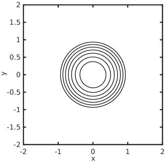
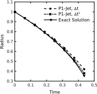
Figure 3: A circle collapsing under mean curvature flow using a P1-Jet with $h=0.125$ and $dt=4h^{2}$. (a) The interface location is shown at intervals of $\Delta t$ until $t=0.375$. (b) A comparison between the radius over time using a P1-Jet with different time discretization methods.

4.1.1 Convergence Study

The overall accuracy of the method is a combination of the semi-Lagrangian and semi-implicit methods,

$$\mathcal{O}(\Delta t^{k})+\mathcal{O}\big{(}\frac{h^{p+1}}{\Delta t}\big{)}+\mathcal{O}(h^{L}),$$ (50)

where $\Delta t$ is the time step, $h$ is the grid spacing, $k$ is the time step order, $p$ is the order of the interpolant, and $L$ is the accuracy order at which the smoothing operator is discretized. Here $k=1$ or $k=2$, $p=3$, and $L=2$. Clearly, there will be trade-off in accuracy as the time step is reduced. Given a fixed grid spacing it should be expected that at large time steps the error will be dominated by the time-integration error, $\mathcal{O}(\Delta t^{k})$, and as such should decrease at a rate dictated by the time step order. As the time step decreases the error begins to be dominated by the smoothing term, $\mathcal{O}(h^{L})$, if $L<p+1$. A further decrease in the time step results in the interpolation error, $\mathcal{O}(h^{p+1}/\Delta t)$, dominating and any further decrease in the time step will result in an increase in the error.

Therefore there are three convergence regions with respect to the time step which are to be expected. The first is a decrease at the rate of $\mathcal{O}(\Delta t^{k})$, the second will be a relatively constant error region dictated by $\mathcal{O}(h^{L})$, and the final will be an increase in the error at a rate of $\mathcal{O}(h^{p+1}/\Delta t)$. Note that the $1/\Delta t$ is included to account for the fact that interpolation is performed about $1/\Delta t$ times during the course of a simulation. This is not a unique occurrence and has been observed in other instances of semi-Lagrangian time integration [33, 34].

To verify this accuracy a two-dimensional circle shrinking under mean curvature flow is compared to the analytic solution. A circle with an initial radius of 1 centered at the origin is allowed to evolve until a time of $T=0.375$, at which point the error is calculated. Define the error at a point on the interface as $e(x_{\Gamma},y_{\Gamma},t)=|\sqrt{x_{\Gamma}^{2}+y_{\Gamma}^{2}}-r(t)|$, where $(x_{\Gamma},y_{\Gamma})$ is a point on the interface and $r(t)=\sqrt{r_{0}^{2}-2t}$ is the analytic radius. The overall error is the $L_{\infty}$-error defined over all closest points calculated at $T=0.375$. This error definition tests not only the time-evolution of the Jet but also the recovery of the interface by way of the cubic interpolation function.

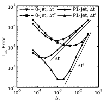
(a) $h=0.0625$

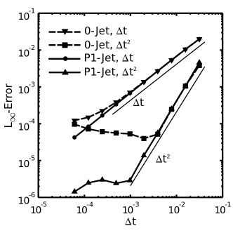
(b) $h=0.015625$

Figure 4: Comparison of a 0-Jet with a P1-Jet using both $\mathcal{O}(\Delta t)$ and $\mathcal{O}(\Delta t^{2})$ in time methods for (a) $h=0.0625$ and (b) $h=0.015625$.

The first error-convergence results are for fixed grid spacings of $h=0.0625$ and $h=0.015625$, Fig. 4. In this figure both a 0-Jet and a P1-Jet are used with $\mathcal{O}(\Delta t)$ and $\mathcal{O}(\Delta t^{2})$ in time methods. Initially the error converges based on the underlying time integration, $\mathcal{O}(\Delta t^{k})$. As the time step decreases the $\mathcal{O}(h^{2})$ terms begin to dominate and approximately constant error regions are observed, particularly for the P1-Jet using second-order time discretization in Fig. 4(b). As the time step further decreases the dominate term becomes $\mathcal{O}\big{(}h^{4}/\Delta t\big{)}$ and the error increases with a further decrease in the time step. This is clearly seen in the error plot of the coarser mesh, Fig. 4(a). Both the $\mathcal{O}(\Delta t)$ and $\mathcal{O}(\Delta t^{2})$ methods have roughly the same error at small time steps as that error is completely dominated by the interpolation error. For the finer mesh, Fig. 4(b), the integration error is smaller and therefore this increase at small time steps is delayed. In general the P1-Jet provides more accurate results at moderate and large time steps. Only at small time steps, when the integration error begins to dominate, does the 0-Jet have slightly smaller error. The exact cause of this reversal is not known, but could be due to some fortuitous cancelation.

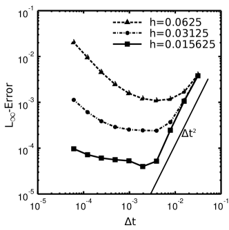
(a) 0-Jet

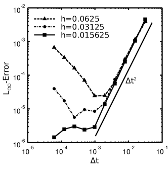
(b) P1-Jet

Figure 5: Error dependence on the time step size for different grid sizes. The time-integration scheme is $\mathcal{O}(\Delta t^{2})$.

To further explore the influence of the Jet and of the smoothing operator the error as a function of time step is investigated for different Jets and grid spacings, Fig. 5. At large time steps the error is completely dominated by the time-integration term, and therefore no difference can be observed between the different grid spacings, particularly for the P1-Jet, Fig. 5(b). As the grid spacing is decreased the minimum error over all time steps decreases at a rate of $\mathcal{O}(h^{2})$, see Table 1. This indicates that for large time steps any spatial errors are dominated by the smoother operator, not the integration error. This is to be expected so long as $\Delta t>h$, which results in an overall integration error of $\mathcal{O}(h^{3})$.

Table 1: The smallest $L_{\infty}$-error of the interface for the circle under mean curvature flow over all time steps. The overall minimum error is dominated by the accuracy of the smoothing operation.

$h$	0-Jet $L_{\infty}$	0-Jet Order	P1-Jet $L_{\infty}$	P1-Jet Order
0.0625	$1.15\times 10^{-3}$	—	$2.43\times 10^{-5}$	—
0.03125	$2.45\times 10^{-4}$	2.23	$5.61\times 10^{-6}$	2.13
0.015625	$4.03\times 10^{-5}$	2.6	$1.43\times 10^{-6}$	1.96

4.1.2 Cassini Oval

The extension of the SemiJet method to three dimensions is demonstrated by considering the collapse of a Cassini oval under mean-curvature flow, Fig. 6. The initial shape of the interface is given by $\tilde{\phi}=((x-a)^{2}+y^{2}+z^{2})((x+a)^{2}+y^{2}+z^{2})-b^{4}$ with $a=1.29$ and $b=1.3$ using a grid spacing of $h=0.0634$. This is then replaced by a signed-distance function by reinitialization. The surface of the Cassini moves inward and the neck region narrows as the surface shrinks. As time goes on the Cassini pinches off at the middle and splits into two separate interfaces. The method has been tested using large time steps and works reliably. However, the pinch-off dynamics are very rapid and thus to capture the topological changes the time step is chosen to be $\Delta t=h^{2}$. This example also shows that the use of a P1-Jet does not destroy the ability of level set methods to capture topological changes.

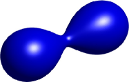
(a) t=0

(b) t=0.0605

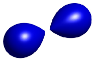
(c) t=0.0645

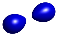
(d) t=0.0806

Figure 6: Collapse of a three-dimensional Cassini oval under mean curvature flow for $h=0.0634$ and $\Delta t=h^{2}$ using a P1-Jet with second order time discretization.

A comparison between the 0-Jet and P1-Jet for a collapsing Cassini oval is shown in Fig. 7. As can be seen the neck using the 0-Jet is thicker than the P1-Jet at the same time. This indicates that the 0-Jet is under-reporting the curvature, leading to a delay in splitting time.

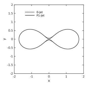
(a) Comparison of a 0-Jet with a P1-Jet

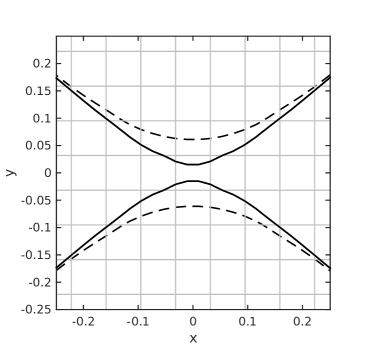
(b) Close-up view of the neck region. 0-Jet under-reports the curvature without the higher accuracy afforded by P1-Jet

Figure 7: Cross-section of the $x-y$-plane of the Cassini Oval using a 0-Jet and P1-Jet at a time of $t=0.0605$. The neck region of the 0-Jet is thicker than the P1-Jet.

In Fig. 8 the ability of the P1-Jet to capture sub-grid information is demonstrated. Here, a comparison is made between interfaces constructed with three different interpolation approaches for the collapsing Cassini oval at a time of $t=0.0605$. The solid black lines represents the interface constructed using the P1-Jet information to determine the cubic interpolant. This result is the same as Fig. 7(b). This is denoted as a sub-grid structure due to the fact that two interface crossings occur on a cell edge where $\phi>0$ on both of the cell corners. Compare this to a cubic interpolant determined using only the level set values and approximating the derivatives from finite difference approximations, the dashed line in Fig. 8. In this case the center region is completely split. Finally, consider the case of using linear interpolation with only the level set values, the dash-dot line in Fig. 8. The description of the interface using linear interpolation is even worse, with only straight lines being described. This demonstrates that the tracking of level set derivatives is beneficial in describing the interface.

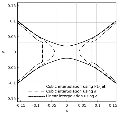
Figure 8: Close-up view of the Cassini Oval at t = 0.0605 showing sub-grid structure. The neck region falls within a grid cell (represented by solid black lines) which is captured by P1-Jet through the locally available gradient information

4.2 Volume-Conserving Mean Curvature Flow

In volume-conserving mean curvature flow the velocity of the interface is given by $\boldsymbol{u}=-(\kappa-\kappa_{avg})\boldsymbol{n}$ where $\kappa$ is the mean curvature, $\boldsymbol{n}$ is the outward normal to the interface and $\kappa_{avg}$ is the average mean curvature on the interface given by

$$\kappa_{avg}=\frac{\int_{\Gamma}\kappa\;\mathrm{d}a}{\int_{\Gamma}\;\mathrm{d}a}\approx\frac{\int_{\Omega}\kappa\;\delta(\phi)\;\|\nabla\phi\|\;\mathrm{d}\boldsymbol{x}}{\int_{\Omega}\delta(\phi)\;\|\nabla\phi\|\;\mathrm{d}\boldsymbol{x}},$$ (51)

where $\Omega$ is the computational domain and $\delta(\phi)$ is a Dirac delta function [35]. Under this velocity field the interface will evolve into a single circle in 2D and sphere in 3D, where the average curvature equals the local curvature.

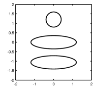
(a) t=0

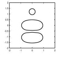
(b) t=0.10

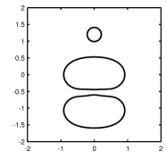
(c) t=0.12

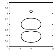
(d) t=0.15

Figure 9: Volume-conserving mean curvature flow in two dimensions using a 0-Jet. The grid spacing is $h=0.0634$ while the time step is $\Delta t=0.5h^{2}$. At $t=0.15$ the volume change is 1.35%.

The first test case is a two-dimensional system containing two ellipses and a circle subjected to volume conserving mean curvature flow. As the curvature is a quantity local to each interface, ideally all interfaces would evolve independently until they merge. Provided enough time the final shape of the interface will become a circle. Results for both a 0-Jet, Fig. 9, and P1-Jet, Fig. 10, are provided. The volume loss for the 0-Jet is 1.35% while that for the P1-Jet is 1.28%.

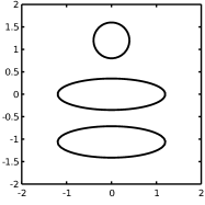
(a) t=0

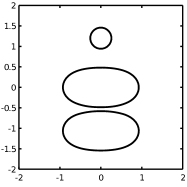
(b) t=0.10

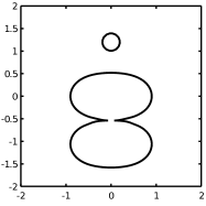
(c) t=0.12

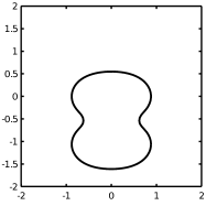
(d) t=0.15

Figure 10: Volume-conserving mean curvature flow in two dimensions using a P1-Jet. The grid spacing is $h=0.0634$ while the time step is $\Delta t=0.5h^{2}$. At $t=0.15$ the volume change is 1.28%.

While the volume conservation is similar it is clear that the 0-Jet result is incorrect. It has been previously observed that the non-local nature of the semi-implicit level set method results in the incorrect behavior of near-by interfaces [12, 16]. This is due to the difficulty in calculating the curvature when two interfaces are near each other [36, 37]. This can be clearly observed in the 0-Jet time-evolution, where the interfaces are clearly distorted and have not yet merged at $t=0.15$, Fig. 9. Contrast that with the P1-Jet, where much less interface distortion is observed and the interfaces are fully merged at $t=0.15$. While the curvature calculation is non-local to the interface using the curvature calculation described earlier, the higher accuracy, as demonstrated by the results in previous sections, reduces the influence of nearby interfaces.

A comparison between the original, explicit Jet scheme is also made to the presented SemiJet method by considering the volume-conserving mean-curvature flow of a three-dimensional star shape, Fig. 11. Under this motion any given initial shape will eventually become a sphere. Using the original Jet scheme oscillations begin to appear on the interface, which will lead to numerical failure due to incorrect curvature calculation. Numerical experiments show that the instability of the original Jet scheme becomes more severe over time and the solution eventually breaks down. The presented SemiJet method is able to maintain a smooth interface through the entire time with the same time step with only a volume change of 0.37%.

(a) $t=0$

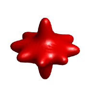
(b) $t=0.05$

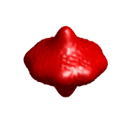
(c) $t=0.11$

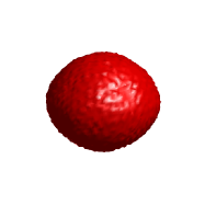
(d) $t=0.58$

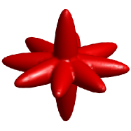
(e) $t=0$

(f) $t=0.05$

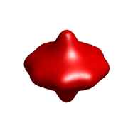
(g) $t=0.11$

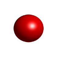
(h) $t=0.58$

Figure 11: A comparison of the original Jet ($\beta=0$) method, (a)-(d), with the SemiJet, (e)-(h), showing the volume-conserving mean curvature flow of a three dimensional star with $\Delta t=1.5h^{2}$ and $h=0.0625$. Both solutions use a P1-Jet. Using the original Jet method oscillations on the interface grow over time, leading to the eventual failure of the simulation. The SemiJet scheme, on the other hand, maintains a smooth solution at all times. Using the SemiJet volume loss is about 0.37% at $t=0.58$.

4.3 Qualitative Stability Analysis

In this section the stability of the SemiJet method (P1-Jet with $\beta=0.5$) is compared to the original semi-implicit level set method (0-Jet with $\beta=0.5$) and the original Jet scheme (P1-Jet with $\beta=0$). Consider a two-dimensional circle under volume-conserving mean curvature flow, $\boldsymbol{u}=-(\kappa-\kappa_{avg})\boldsymbol{n}$. In the ideal case the interface will not move due to the local curvature being equal to the average curvature over the interface. This situation can be used to investigate the stability of the underlying numerical scheme. As the interface should not move any motion of the interface will be due to errors when calculating the curvature and advecting the interface. If the time step is too large for a given numerical method these errors will compound resulting in the eventual failure of the simulation.

To test the stability various numerical simulations are carried out to determine the maximum stable time step for various combinations of Jet-order, time step accuracy order, and amount of smoothing. While the amount of volume change during the course of a simulation is small over reasonable time steps, as demonstrated above, during large time steps the volume change can become excessive. To minimize the influence of this volume change on the determination of the maximum stable time step a volume correction procedure is performed. After every time step the level set is shifted by $\left(V_{n}-V_{0}\right)/A_{n}$, where $V_{n}$ is the current volume, $V_{0}$ is the initial volume, and $A_{n}$ is the current area of the interface. In 2D these are replaced with the current area, initial area, and current interface length, respectively.

A time step is determined to result in a stable simulation if the following conditions are satisfied: 1) the simulation can run for 1000 time steps and 2) the difference between the maximum and minimum velocity over the last 100 iterations is less than 10% of the minimum velocity over the 1000 total time steps. Sample velocity profiles over 1000 iterations for a 0-Jet using $\beta=0.5$ with second-order accurate time discretization for three different time steps is shown in Fig. 12. There are three types of behaviors observed. The first is an unstable time step, where the simulation is not able to complete 1000 iterations before failing due to excessive numerical errors. The second type is a semi-stable time step, where the simulation completes 1000 iterations but the velocity is slowly increasing. This indicates that the simulation will fail at some point in the future. Finally, a stable time is one which completes all 1000 iterations and the velocity is stable. A stable time step will not have zero velocity; instead any small movement of the interface is adjusted by the volume-correction procedure.

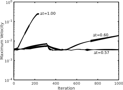
Figure 12: The maximum velocity using three different time steps using a 0-Jet with $\beta=0.5$ for a unit circle under volume-conserving mean curvature flow. Three types of behaviors are shown. An unstable time step ($\Delta t=1.00$) does not complete 1000 iterations. A semi-stable time step ($\Delta t=0.60$) completes the 1000 iterations but the velocity is slowly increasing over time. A stable time step ($\Delta t=0.57$) completes 1000 iterations and the velocity remains constant.

The maximum possible stable time step is reported in Table 2 for a two-dimensional unit circle with volume-conserving mean curvature flow on a grid with $h=0.0625$. While this determination of a stable time step is qualitative in nature it does provide insight into the overall stability properties of the SemiJet method. It is clear that the explicit scheme, given by $\beta=0$, is restricted by the standard CFL condition of $\Delta t\leq h^{2}$. The application of a smoothing operator, given by $\beta=0.5$, relaxes this constraint. In the case of a P1-Jet and first-order time discretization the maximum possible time step is over 400-times that of $h^{2}$.

Table 2: The largest stable time step for various combinations of the Jet, time step order, and smoothing on a grid with $h=0.0625$. The explicit Jet method is given by $\beta=0$ while the SemiJet method is given by $\beta=0.5$.

		$\beta=0$		$\beta=0.5$
Jet Order	Time Order	$\Delta t_{max}$	$\Delta t_{max}/h^{2}$	$\Delta t_{max}$	$\Delta t_{max}/h^{2}$
0	1	0.00205	0.52	0.98	251
P1	1	0.00375	0.96	1.71	438
0	2	0.00135	0.35	0.57	146
P1	2	0.00245	0.63	0.79	179

It is interesting to note that in all cases the use of a P1-Jet results in a more stable scheme than the 0-Jet. This holds true for both the explicit case, $\beta=0$, and the semi-implicit case, $\beta=0.5$. It is suspected that the averaging of the derivatives when calculating the curvature in the P1-Jet case is partially responsible for this increase in stability. It should also be noted that in general a first-order time discretization scheme is more stable than the second-order schemes. This is due to the extrapolation step during the second-order time discretization. Any oscillations in the velocity field will be magnified when extrapolating into the future.

4.4 Computational Cost Comparison

In this section the computational cost of the proposed SemiJet method is compared to a standard fifth order upwind WENO method. The first test case considered here is the collapse of a two-dimensional unit circle under mean curvature flow, $\boldsymbol{u}=-\kappa\boldsymbol{n}$. The system is allowed to run until $t=0.375$, at which time the error is computed, see Sec. 4.1 for more details. The domain spans the $[-2,2]^{2}$ square. During the simulation the wall-clock time spent in the evolution of the level-set or Jet is determined. Note that operations common to different cases, such as reinitialization, are not included in the timings. This was done to ensure that an accurate comparison between methods is performed. All simulations were performed using 8 AMD Opteron 6320 cores.

The WENO method is discretized using a second-order backward-finite-difference method in time and second-order extrapolation of the velocity in time:

$$\dfrac{3\phi_{n+1}-2\phi_{n}+\phi_{n-1}}{2\Delta t}+2\boldsymbol{u}_{n}\cdot\nabla\phi_{n}-\boldsymbol{u}_{n-1}\cdot\nabla\phi_{n-1}=0,$$ (52)

where the gradients are discretized using a fifth-order upwind WENO scheme [38]. Note that when using the WENO scheme, only the level-set field is tracked. The Jet (with $\beta=0$) and SemiJet (with $\beta=0.5$) both utilize a P1-Jet. As $\beta=0$ for the Jet, it is an explicit scheme in time, and thus both the WENO and Jet schemes will be under strict stability constraints, see Sec. 4.3 for a qualitative stability analysis of of the Jet scheme. It is expected that WENO will obey similar restrictions. The results are presented in Table 3. For the WENO and Jet methods the time step is set to $0.25h^{2}$, while with the SemiJet method a larger time step can be used.

Table 3: The $L_{\infty}$ error and wall-clock time required to model a two-dimensional circle collapsing under mean-curvature flow until a time of $t=0.375$.

Method	Grid Size	Time Steps	$\Delta t/h^{2}$	$L_{\infty}$ Error	Elapsed Time (s)
WENO	257	6144	0.25	$6.81\times 10^{-3}$	99.53
WENO	129	1536	0.25	$1.33\times 10^{-2}$	6.38
WENO	65	384	0.25	$2.54\times 10^{-2}$	0.42
Jet	257	6144	0.25	$2.03\times 10^{-6}$	1527
Jet	129	1536	0.25	$1.06\times 10^{-5}$	91.95
Jet	65	384	0.25	$4.68\times 10^{-5}$	5.95
SemiJet	257	6144	0.25	$2.41\times 10^{-6}$	2377
SemiJet	257	250	6.14	$6.82\times 10^{-6}$	98.36
SemiJet	257	24	64	$1.04\times 10^{-3}$	10.50
SemiJet	129	1536	0.25	$1.94\times 10^{-5}$	148.8
SemiJet	129	48	8	$2.91\times 10^{-4}$	4.76
SemiJet	129	24	16	$1.07\times 10^{-3}$	2.45
SemiJet	65	384	0.25	$6.87\times 10^{-5}$	9.91
SemiJet	65	12	8	$3.91\times 10^{-3}$	0.35
SemiJet	33	12	2	$4.33\times 10^{-3}$	0.12

It is clear from the results that the Jet and SemiJet are much more costly than the WENO scheme for the same grid size and time step, with the Jet being approximately 15 times more expensive and the SemiJet approximately 23 times more expensive. This is due to the fact that for every grid point, four sub-grid points (in 2D) must be updated. Each of these updates requires not only determining the departure location, but also the evaluation of multiple cubic interpolants. Note that no effort was made to optimize this interpolation, and thus some time savings could be gained there.

The results also indicate, though, that the quality of the solution, as measured by the $L_{\infty}$ error, is much better for the Jet and SemiJet schemes as compared to the WENO method. For the same grid size and time step, the Jet and SemiJet schemes are between two- and three-orders of magnitude more accurate than the WENO scheme. For the SemiJet scheme, this allows for an increase in the time step to still produce an accurate result. For example, using a grid size of $257^{2}$ (grid spacing of $1.5625\times 10^{-2}$) the WENO result has an error of $6.81\times 10^{-3}$. The same computational cost ($\sim 100$ s) can be achieved with the SemiJet scheme using a time step 24 times larger than the WENO case. Even with this larger time step, the error for the SemiJet case is three orders of magnitude smaller, $6.82\times 10^{-6}$ for the SemiJet scheme. Using the SemiJet scheme with a time step 256 times larger ($\Delta t=1.563\times 10^{-2}$) than the WENO one for the same grid results in a scheme which is 6.5 times more accurate but only takes one-tenth of the time, 10.5 s versus 99.53 s.

This behavior, that at the same computational cost the SemiJet scheme is much more accurate than the WENO scheme is consistent across multiple grid sizes. In fact, using an extremely coarse grid spacing of 0.125, corresponding to a $33^{2}$ grid, with a very large time step still results in a more accurate result than the WENO scheme with a fine grid and very small time step, in a computational time which is 830 times faster. This behavior is consistent with that shown by Chidyagwai et al. for linear advection [9].

The second test case is mean curvature flow in three dimensions, $\boldsymbol{u}=-0.5\kappa\boldsymbol{n}$, where $\kappa$ represents the sum of the principle curvatures. In this case the size of the grid is fixed at $129^{3}$ over a cube spanning $[-2,2]^{3}$. These simulations were performed using 128 AMD Opteron 6320 cores, with the results seen in Table 4.

Table 4: The $L_{\infty}$ error and wall-clock time required to model a three-dimensional sphere collapsing under mean-curvature flow until a time of $t=0.375$. All cases use a $129^{3}$ grid.

Method	Time Steps	$\Delta t/h^{2}$	$L_{\infty}$ Error	Elapsed Time (s)
WENO	1536	0.25	$2.43\times 10^{-2}$	77.33
Jet	1536	0.25	$1.14\times 10^{-4}$	2022
SemiJet	1536	0.25	$1.21\times 10^{-4}$	3417
SemiJet	48	8	$2.73\times 10^{-4}$	116.9
SemiJet	30	12.8	$6.29\times 10^{-4}$	73
SemiJet	24	16	$9.65\times 10^{-4}$	60.15
SemiJet	12	32	$3.63\times 10^{-3}$	32.44

The results for the three-dimensional case are similar to those for the two-dimensional one. Here, the Jet is approximately 26 times more expensive and the SemiJet is approximately 44 times more expensive than the WENO scheme for the same grid size. In three-dimensions there are eight sub-grid points that need to be updated, which explains the increase over the two-dimensional results. Similar to the two-dimensional case, the Jet and SemiJet schemes are two orders of magnitude more accurate than the WENO scheme at the same grid size and time-step. Using the SemiJet method with 30 time steps, corresponding to $\Delta t=0.0125$, results in the same computational cost as the WENO method but a result which is 40 times more accurate. In fact, using an extremely coarse $33^{3}$ mesh with a time step of $\Delta t=0.125$ on two cores results in an elapsed time of 21 s and an error of $3.05\times 10^{-3}$, which is both faster and more accurate than the WENO case, using much fewer computational resources.

5 Summary and Conclusion

In this work a robust numerical method, the SemiJet, is presented for moving interface problems with numerically-stiff velocity fields. The method builds upon the original Jet scheme developed by Seibold et al. and the semi-implicit level set method of Smereka. The influence of the semi-implicit smoothing operation is captured by defining a smoothing source term, which is then used when updating the derivative fields in the level set Jet. The results demonstrate that the use of a Jet increases both the accuracy and stability of the simulations over both the original Jet and original semi-implicit level set methods. Unlike the previous SIGALS method only one smoothing operation is required and the use of the $\epsilon$-finite different method allows for straight-forward extension to higher order jet schemes. While the SemiJet method is computationally more expensive than a WENO scheme for the same grid and time step, the added stability and accuracy allows for smaller grid sizes and larger time steps to be used, which results in methods with overall higher efficiency and accuracy.

References

References

- [1] J. A. Sethian, P. Smereka, Level Set Methods For Fluid Interfaces, Annual Review of Fluid Mechanics 35 (1) (2003) 341–372.
- [2] R. Malladi, J. Sethian, Image Processing Via Level Set Curvature Flow, Proceedings of the National Academy of Sciences of the United States of America 92 (15) (1995) 7046–50.
- [3] S. Chen, B. Merriman, S. Osher, P. Smereka, A Simple Level Set Method for Solving Stefan Problems, Journal of Computational Physics 135 (1) (1997) 8–29.
- [4] M. Y. Wang, X. Wang, D. Guo, A Level Set Method For Structural Topology Optimization, Computer Methods in Applied Mechanics and Engineering 192 (1-2) (2003) 227–246.
- [5] J.-C. Nave, R. R. Rosales, B. Seibold, A Gradient-Augmented Level Set Method With an Optimally Local, Coherent Advection Scheme, Journal of Computational Physics 229 (10) (2010) 3802–3827.
- [6] D. Kolomenskiy, J.-C. Nave, K. Schneider, Adaptive Gradient-Augmented Level Set Method with Multiresolution Error Estimation, Journal of Scientific Computing (2014) 1–25.
- [7] C. Lee, J. Dolbow, P. J. Mucha, A Narrow-Band Gradient-Augmented Level Set Method for Multiphase Incompressible Flow, Journal of Computational Physics 273 (2014) 12–37.
- [8] B. Seibold, J.-C. Nave, R. R. Rosales, Jet Schemes For Advection Problems, Discrete and Continuous Dynamical Systems - Series B 17 (4) (2012) 1229–1259.
- [9] P. Chidyagwai, J.-C. Nave, R. R. Rosales, B. Seibold, A Comparative Study Of The Efficiency Of Jet Schemes, Int.J. Numer. Anal. Model.-B 3 (3) (2012) 297–306.
- [10] M. Sussman, P. Smereka, S. Osher, A Level Set Approach for Computing Solutions to Incompressible Two-Phase Flow, Journal of Computational Physics 114 (1) (1994) 146–159.
- [11] S. Hysing, A New Implicit Surface Tension Implementation for Interfacial Flows, International Journal for Numerical Methods in Fluids 51 (6) (2006) 659–672.
- [12] D. Salac, W. Lu, A Local Semi-implicit Level-set Method For Interface Motion, Journal of Scientific Computing 35 (2-3) (2008) 330–349.
- [13] S. Popinet, An Accurate Adaptive Solver For Surface-Tension-Driven Interfacial Flows, Journal of Computational Physics 228 (16) (2009) 5838–5866.
- [14] D. Salac, M. Miksis, A Level Set Projection Model of Lipid Vesicles in General Flows, Journal of Computational Physics 230 (22) (2011) 8192–8215.
- [15] E. M. Kolahdouz, D. Salac, A Semi-Implicit Gradient Augmented Level Set Method, SIAM Journal on Scientific Computing 35 (1) (2013) A231–A254.
- [16] P. Smereka, Semi-Implicit Level Set Methods for Curvature and Surface Diffusion Motion, Journal of Scientific Computing 19 (2003) 439–456.
- [17] E. M. Kolahdouz, D. Salac, Dynamics of Three-Dimensional Vesicles in DC Electric Fields, Phys. Rev. E 92 (2015) 012302.
- [18] E. M. Kolahdouz, D. Salac, Electrohydrodynamics of Three-Dimensional Vesicles: A Numerical Approach, SIAM Journal on Scientific Computing 37 (3) (2015) B473–B494.
- [19] L. Duchemin, J. Eggers, The Explicit–Implicit–Null method: Removing the numerical instability of PDEs, Journal of Computational Physics 263 (2014) 37–52.
- [20] M. Burger, Numerical simulation of anisotropic surface diffusion with curvature-dependent energy, Journal of Computational Physics 203 (2) (2005) 602–625.
- [21] E. Olsson, G. Kreiss, A conservative level set method for two phase flow, Journal of Computational Physics 210 (1) (2005) 225–246.
- [22] C. Kublik, N. M. Tanushev, R. Tsai, An implicit interface boundary integral method for Poisson’s equation on arbitrary domains, Journal of Computational Physics 247 (2013) 279–311.
- [23] X.-D. Liu, R. P. Fedkiw, M. Kang, A Boundary Condition Capturing Method for Poisson’s Equation on Irregular Domains, Journal of Computational Physics 160 (1) (2000) 151–178.
- [24] D. Peng, A PDE-Based Fast Local Level Set Method, Journal of Computational Physics 155 (2) (1999) 410–438.
- [25] D. L. Chopp, Some Improvements of the Fast Marching Method, SIAM Journal on Scientific Computing 23 (1) (2001) 230–244.
- [26] A. Kumar, Isotropic Finite-Differences, Journal of Computational Physics 201 (1) (2004) 109–118.
- [27] M. Patra, M. Karttunen, Stencils with Isotropic Discretization Error for Differential Operators, Numerical Methods for Partial Differential Equations 01794.
-
[28]
S. Balay, S. Abhyankar, M. F. Adams, J. Brown, P. Brune, K. Buschelman,
L. Dalcin, V. Eijkhout, W. D. Gropp, D. Kaushik, M. G. Knepley, L. C.
McInnes, K. Rupp, B. F. Smith, S. Zampini, H. Zhang,
PETSc Web page,
http://www.mcs.anl.gov/petsc (2015).
URL http://www.mcs.anl.gov/petsc -
[29]
S. Balay, S. Abhyankar, M. F. Adams, J. Brown, P. Brune, K. Buschelman,
L. Dalcin, V. Eijkhout, W. D. Gropp, D. Kaushik, M. G. Knepley, L. C.
McInnes, K. Rupp, B. F. Smith, S. Zampini, H. Zhang,
PETSc Users Manual, Tech. Rep.
ANL-95/11 - Revision 3.6, Argonne National Laboratory (2015).
URL http://www.mcs.anl.gov/petsc - [30] S. Balay, W. D. Gropp, L. C. McInnes, B. F. Smith, Efficient Management of Parallelism in Object Oriented Numerical Software Libraries, in: E. Arge, A. M. Bruaset, H. P. Langtangen (Eds.), Modern Software Tools in Scientific Computing, Birkhäuser Press, 1997, pp. 163–202.
- [31] L. Anumolu, M. F. Trujillo, Gradient augmented reinitialization scheme for the level set method, International Journal for Numerical Methods in Fluids 73 (12) (2013) 1011–1041.
- [32] L.-T. Cheng, Y.-H. Tsai, Redistancing by Flow of Time Dependent Eikonal Equation, Journal of Computational Physics 227 (8) (2008) 4002–4017.
- [33] J. Strain, Semi-Lagrangian Methods For Level Set Equations, Journal of Computational Physics 151 (2) (1999) 498–533.
- [34] D. Xiu, G. E. Karniadakis, A Semi-Lagrangian High-order Method For Navier–stokes Equations, Journal of computational physics 172 (2) (2001) 658–684.
- [35] J. D. Towers, A Convergence Rate Theorem for Finite Difference Approximations to Delta Functions, Journal of Computational Physics 227 (13) (2008) 6591–6597.
- [36] P. Macklin, J. Lowengrub, An Improved Geometry-Aware Curvature Discretization For Level Set Methods: Application To Tumor Growth, journal of Computational Physics 215 (2) (2006) 392–401.
- [37] K. Y. Lervåg, B. Müller, S. T. Munkejord, Calculation of the Interface Curvature and Normal Vector with the Level-Set Method, Computers & Fluids 84 (2013) 218–230.
- [38] G. Jiang, D. Peng, Weighted ENO schemes for Hamilton-Jacobi equations, SIAM Journal on Scientific Computing 21 (6) (2000) 2126–2143.