Shadow of a Colossus: A $z=2.45$ Galaxy Protocluster Detected
in 3D Ly$\alpha$ Forest Tomographic Mapping of the COSMOS Field

Abstract

Using moderate-resolution optical spectra from 58 background Lyman-break galaxies and quasars at $z\sim 2.3-3$ within a $11.5^{\prime}\times 13.5^{\prime}$ area of the COSMOS field ($\sim 1200\,\mathrm{deg}^{-2}$ projected area density or $\sim 2.4\,h^{-1}{\rm\ Mpc}$ mean transverse separation), we reconstruct a 3D tomographic map of the foreground Ly$\alpha$ forest absorption at $2.2<z<2.5$ with an effective smoothing scale of $\epsilon_{\rm 3D}\approx 3.5\,h^{-1}{\rm\ Mpc}$ comoving. Comparing with 61 coeval galaxies with spectroscopic redshifts in the same volume, we find that the galaxy positions are clearly biased towards regions with enhanced IGM absorption in the tomographic map. We find an extended IGM overdensity with deep absorption troughs at $z=2.45$ associated with a recently-discovered galaxy protocluster at the same redshift. Based on simulations matched to our data, we estimate the enclosed dark matter mass within this IGM overdensity to be $M_{\rm dm}(z=2.45)=(9\pm 4)\times 10^{13}\,h^{-1}{\rm\ M}_{\odot}$, and argue based on this mass and absorption strength that it will form at least one $z\sim 0$ galaxy cluster with $M(z=0)=(3\pm 2)\times 10^{14}\,h^{-1}{\rm\ M}_{\odot}$, although its elongated nature suggests that it will likely collapse into two separate clusters. We also point out a compact overdensity of six MOSDEF galaxies at $z=2.30$ within a $r\sim 1\,h^{-1}{\rm\ Mpc}$ radius and $\Delta z\sim 0.006$, which does not appear to have a large associated IGM overdensity. These results demonstrate the potential of Ly$\alpha$ forest tomography on larger volumes to study galaxy properties as a function of environment, as well as revealing the large-scale IGM overdensities associated with protoclusters or other features of large-scale structure.

1. Introduction

The study of high-redshift ($z>2$) galaxy protoclusters is a topic of increasing interest, providing a route to studying galaxy evolution, AGN, plasma physics, and our models of gravity. They are also critical laboratories for understanding the growth of massive galaxy clusters at $z\sim 0$. While many studies have successfully found protoclusters around active supermassive black holes such as radio galaxies or luminous quasars (see Hennawi et al. 2015 and Cooke et al. 2014 for recent examples, or Chiang et al. 2013 for a compilation), it is difficult to tell whether these ‘signpost’ protoclusters are representative of the overall population – which, at least in simulations, shows a wide range of properties.

More uniform, ‘blind’, search techniques are therefore required for unbiased samples of protoclusters. Several such objects have been found serendipitously in photometric or galaxy redshift surveys (e.g., Steidel et al., 2005; Gobat et al., 2011; Cucciati et al., 2014; Yuan et al., 2014; Casey et al., 2015). Searching photometric redshift catalogs (Chiang et al., 2014) is another promising new technique, but is limited to fields with extensive multi-wavelength photometry that enable accurate photometric redshfits. Unfortunately we expect protoclusters to be rare, and surveying large volumes of space with these techniques is expensive.

Recently, Stark et al. (2015b) (hereafter S15) argued that 3D tomographic reconstructions of the intergalactic medium (IGM) Lyman-$\alpha$ (Ly$\alpha$) forest absorption (Pichon et al., 2001; Caucci et al., 2008; Lee et al., 2014a) can be used to efficiently search for protoclusters. A protocluster’s Ly$\alpha$ absorption signature extends over a large region ($r\gtrsim 5\,h^{-1}{\rm\ Mpc}$) allowing it to be mapped by background galaxies separated by several transverse Mpc, corresponding to relatively bright limiting magnitudes ($\lesssim 24.5\,$mag) and therefore accessible to existing 8-10m class telescopes. In fact several studies have already found Ly$\alpha$ absorption associated with protoclusters either in single sightlines (Hennawi et al., 2015) or by stacking multiple background spectra (Cucciati et al. 2014; Hayashino et al. in prep.). Moderate-resolution spectra with careful sightline selection should enable 3D mapping even with modest signal-to-noise ratios (S/N).

In Lee et al. (2014b) (hereafter L14b), we made the first attempt at Ly$\alpha$ forest tomography using a set of 24 background Lyman-break galaxy (LBG) spectra within a $5^{\prime}\times 12^{\prime}$ area in the COSMOS field. This marked the first-ever use of LBGs, instead of quasars, for Ly$\alpha$ forest analysis, and the resulting reconstruction at $2.20<z<2.45$ was the first 3D map of the $z>2$ universe probing Mpc-scale structures. In this paper, as part of the pilot observations for the COSMOS Lyman-Alpha Mapping And Tomography Observations (CLAMATO) survey to map the high-redshift IGM, we extend the L14b map volume by a factor of $\sim 2.5\times$. This volume starts to approach that where we expect to see protocluster candidates in a blind survey: in N-body simulations at $z\sim 2.5$ the comoving number density of halo progenitors which by $z=0$ have masses above $10^{14}\,h^{-1}M_{\odot}$ is $\sim 10^{-5}\,h^{3}\,{\rm Mpc}^{-3}$, or to $10^{-6}\,h^{3}\,{\rm Mpc}^{-3}$ for the progenitors of $3\times 10^{14}\,h^{-1}M_{\odot}$ halos (e.g. Stark et al., 2015b). In the simulations of S15, mock observations with similar sightline density and noise as CLAMATO found more than 3/4 of the protoclusters which would eventually grow to form clusters more massive than $3\times 10^{14}\,h^{-1}M_{\odot}$ at $z=0$ but only 1/5 of the protoclusters which would form $10^{14}\,h^{-1}M_{\odot}$ halos by $z=0$. Our observations probe a volume of $V=5.8\times 10^{4}\,h^{-1}{\rm Mpc}^{3}$ at $2.2<z<2.5$. To the extent that these simulations are accurate, there is a $\sim 10\%$ chance we should find a protocluster in the surveyed volume (see also §5).

Two other developments in the past year lend additional synergy: (i) the first data release of the MOSDEF survey (Kriek et al., 2015, hereafter K15), whose near-infrared (NIR) nebular line redshifts reduce systemic redshift uncertainties hence allowing a cleaner comparison with our tomographic map; and (ii) the discovery of a $z=2.45$ galaxy protocluster within our target field (Diener et al. 2015, hereafter D15; Chiang et al. 2015, hereafter C15).

As we shall see, our tomographic map suggests a complex 3D multi-pronged structure for this protocluster, while also revealing other intriguing structures. We also find that galaxies co-eval with our map preferentially inhabit higher absorption regions of the IGM, suggesting that Ly$\alpha$ tomography does indeed probe the underlying large scale structure.

This paper is organized as follows: we describe the data in Section 2 and tomographic reconstruction of the foreground IGM in Section 3, and then describe simulations used for the subsequent analysis (Section 4). Section 5 then describes the protoclusters and overdensities found within our map volume.

In this paper, we assume a concordance flat $\Lambda$CDM cosmology, with $\Omega_{M}=0.27$, $\Omega_{\Lambda}=0.73$ and $H_{0}=70\,~{}{\rm km~{}s}^{-1}\,\mathrm{Mpc}^{-1}$.

2. Observations

We targeted $2.3<z<3$ galaxies and AGN within the COSMOS field (Scoville et al., 2007; Capak et al., 2007) in order to probe the foreground IGM Ly$\alpha$ forest absorption at $z\sim 2.3$. Top priority was given to objects with confirmed redshifts from the zCOSMOS-Deep (Lilly et al., 2007) and VUDS (Le Fèvre et al., 2015) spectroscopic surveys, while we also, where available, added grism redshift information kindly provided by the 3D-HST team (e.g. Brammer et al., 2012). We also selected targets based on photometric redshifts from Ilbert et al. (2009) as well as Salvato et al. (2011) for X-ray detected sources, which have $\sigma_{z}/(1+z)\approx 0.03$ and $<10\%$ catastropic failure rate. This target selection process was carried out in February 2014, prior to the publications by Diener et al. (2015) and Chiang et al. (2015) reporting galaxy overdensities in the field.

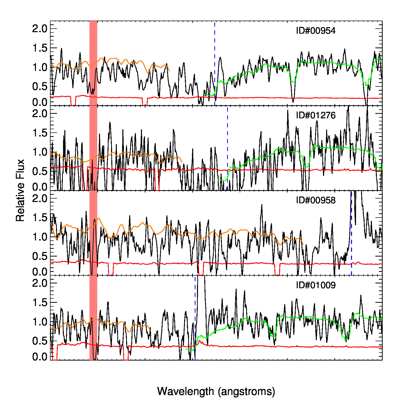
Figure 1.— Examples of galaxy spectra used for our tomographic reconstruction (smoothed by a 3-pixel boxcar for clarity), along with the estimated pixel noise in red, with masked pixels set to zero. The Ly$\alpha$ wavelength at the galaxy redshift is indicated by the vertical dashed-lines, while the green curves shows the LBG composite template from Shapley et al. (2003) for comparison. All these background sources probe the known $z=2.44$ protocluster, with the pink shaded region highlighting the Ly$\alpha$ absorption wavelength ($\lambda\approx 4191\,\mathrm{\AA}$) at the protocluster redshift. Strong associated absorption is apparent even in these individual spectra. Orange curves indicate the estimated continuum level for each object. Note that object #00958 (3rd panel from top) has a broad Ly$\alpha$ emission line characteristic of an AGN, but shows strong ISM absorption redwards of Ly$\alpha$ and is thus treated like a galaxy for continuum-fitting.

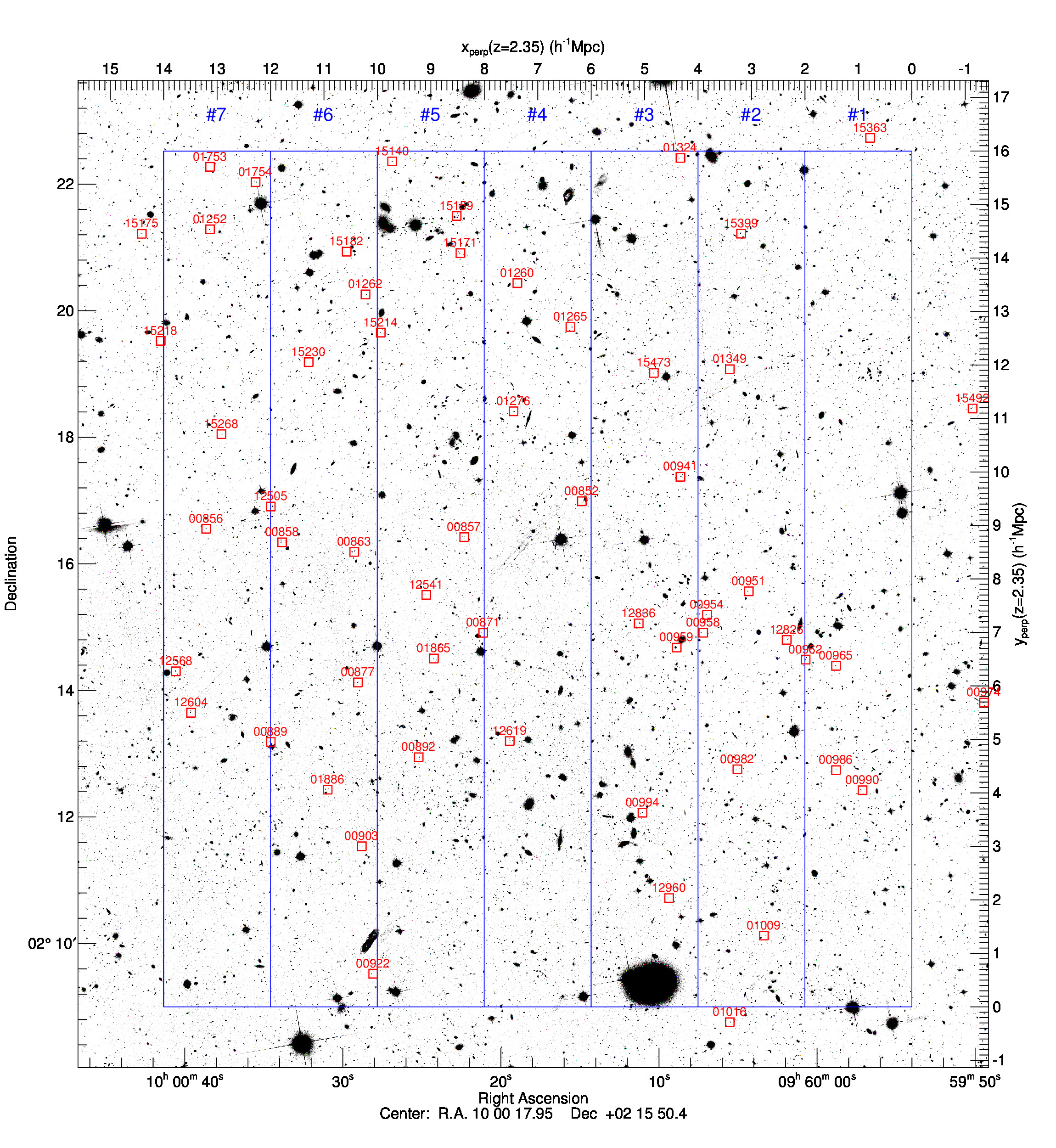
Figure 2.— Hubble ACS image of the COSMOS field (Koekemoer et al., 2007) showing the position of our background galaxies and quasars on the sky, labeled by their ID number. The overall blue box represents the transverse extent of our tomographic map, while the seven narrow slices indicate the footprint of the map projections shown in Figure 4. The upper- and right-axis labels denote the transverse comoving distance at $z=2.35$, the mean redshift of the map.

We observed these targets with the LRIS Double-Spectrograph (Oke et al., 1995; Steidel et al., 2004) on the Keck-I telescope at Maunakea, Hawai’i, during 2014 March 26-27/29-30 and 2015 April 18-20, using multi-object slitmasks. We used the B600/4000 grism on the blue arm and R400/6000 grating on the red with the d560 dichroic, although we work only with the blue spectra in this study. With our $1^{\prime\prime}$ slits, this yields $R\equiv\lambda/\Delta\lambda\approx 1000$, which corresponds to a line-of-sight FWHM of $\approx 3.2\,h^{-1}{\rm\ Mpc}$ at $z\sim 2.3$. Despite inclement weather, we managed $\sim 15$hrs on-target, observing 7 overlapping masks with 7200-9000s exposure times. The observations were mostly carried out in $0.5-1^{\prime\prime}$ seeing, although one mask was observed in $\approx 1.4^{\prime\prime}$ seeing and consequently had a low yield of useable spectra. The data was reduced with the LowRedux package in the XIDL suite of data reduction software, and objects targeted in more than one mask had their spectra co-added. We extracted 162 unique spectra, of which 58 objects had secure visual identifications at redshifts $2.3\lesssim z\lesssim 3.0$ and therefore Ly$\alpha$ forest absorption covering our desired $2.2<z<2.5$ range, as well as adequate S/N ($\mathrm{S/N}\geq 1.3$ per pixel) within the Ly$\alpha$ forest. The majority of these sources are LBGs identified through Ly$\alpha$ emission or intrinsic absorption, although our sample also includes 4 QSOs, one of which is our brightest object ($g=20.12$). The faintest object satisfying our S/N criterion was a $g=25.18$ LBG, although this was observed in two masks; the faintest object from a single mask has $g=24.85$.

Several example spectra are shown in Figure 1, while the source positions are shown in Figure 2. The latter also indicates the $11.8^{\prime}\times 13.5^{\prime}$ footprint of our tomographic map. Within the map footprint, we have 52 background sources which translates to a projected area density of $\sim 1200\,\mathrm{deg}^{-2}$. An additional six sources lie just outside the footprint but will be included in the reconstruction input. The mean transverse separation between the Ly$\alpha$ forest sightlines probing the foreground IGM is $\langle d_{\perp}\rangle\approx 2.4\,h^{-1}{\rm\ Mpc}$.

We next estimate the intrinsic continua, $C$, of the sources. For the quasars, we apply PCA-based mean-flux regulation (MF-PCA; e.g., Lee et al., 2012, 2013a) to the restframe $1041\,\mathrm{\AA}<\lambda<1185\,\mathrm{\AA}$ Ly$\alpha$ forest region using templates from Pâris et al. (2011), masking intrinsic broad absorption where necessary. A similar process is applied on the galaxies, albeit assuming a fixed continuum template from Berry et al. (2012) and adopting a more generous Ly$\alpha$ forest range ($1040\,\mathrm{\AA}<\lambda<1195\,\mathrm{\AA}$). We also mask $\pm 5\,\mathrm{\AA}$ around possible intrinsic absorption at N II $\lambda$1084.0, N I $\lambda$1134.4, and C III $\lambda$1175.7. L14b estimated an rms error of $\sim 10\%$ for the continua, which is adequate considering our noisy spectra.

We then compute the Ly$\alpha$ forest fluctuations, $\delta_{F}$, from the observed spectral flux density, $f$:

$$\delta_{F}=\frac{f}{C\langle F(z)\rangle}-1,$$ (1)

where $\langle F(z)\rangle$ is the mean Ly$\alpha$ transmission from Faucher-Giguère et al. (2008) evaluated at redshift $z$. The $\delta_{F}$ values from our background sources, along with the associated pixel noise errors $\sigma_{N}$ estimated by the reduction pipeline, constitute a sparse sampling of the IGM Ly$\alpha$ forest absorption, which we will reconstruct in the next section.

3. Tomographic Reconstruction

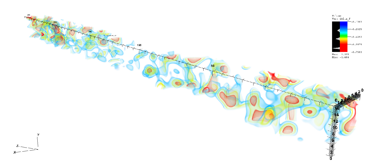
Figure 3.— Three-dimensional visualization of the tomographic reconstruction from our Ly$\alpha$ forest data, which can be viewed as a video online (24MB, https://youtu.be/KeW1UJOPMYI). The $x$- and $y$-dimensions, spanning $14\,h^{-1}{\rm\ Mpc}$ and $16\,h^{-1}{\rm\ Mpc}$ respectively, are on the sky plane (c.f. Figure 2), while the $z$-axis spans $260\,h^{-1}{\rm\ Mpc}$ along the line-of-sight. All axes are in units of $\,h^{-1}{\rm\ Mpc}$ comoving, with the $z$-axis originating at $z=2.20$ and extending to $z=2.50$. Since this map traces Ly$\alpha$ forest transmitted fraction, more negative values correspond to higher-density regions. In the video, first 5 seconds show only the sightline positions before the actual map is revealed.

For the tomographic reconstruction, we define a 3D output grid with cells of comoving size $0.5h^{-1}{\rm\ Mpc}$, spanning a transverse comoving length at $z=2.35$ of $14\,h^{-1}{\rm\ Mpc}$ in the R.A. direction and $16\,h^{-1}{\rm\ Mpc}$ in Dec (Figure 2). The output grid spans $2.2<z_{\alpha}<2.5$ along the line-of-sight, corresponding to $260\,h^{-1}{\rm\ Mpc}$ with our simplification that the comoving distance-redshift relationship is evaluated at fixed $z=2.35$. The overall comoving volume is $V=14\,h^{-1}{\rm\ Mpc}\times 16\,h^{-1}{\rm\ Mpc}\times 260\,h^{-1}{\rm\ Mpc}=58240\,h^{-3}\mathrm{Mpc}^{3}\approx(38.8\,h^{-1}{\rm\ Mpc})^{3}$, i.e. nearly $2.5\times$ greater volume than the L14b map, which corresponds approximately to Slices #5-7 in Figure 2.

As in L14b, we use a Wiener filtering implementation developed by S15. The reconstructed flux field on the output grid is given by

$$\delta_{F}^{\rm rec}=\mathbf{C}_{\mathrm{MD}}\cdot(\mathbf{C}_{\mathrm{DD}}+\mathbf{N})^{-1}\cdot\delta_{F},$$ (2)

where $\mathbf{C}_{\mathrm{DD}}+\mathbf{N}$ and $\mathbf{C}_{\mathrm{MD}}$ are the data-data and map-data covariances, respectively. We assumed a diagonal form for the noise covariance matrix $\mathbf{N}\equiv N_{ii}=\sigma_{N,i}^{2}$, and assumed a Gaussian covariance between any two points $r_{1}$ and $r_{2}$, such that $\mathbf{C}_{\mathrm{DD}}=\mathbf{C}_{\mathrm{MD}}=\mathbf{C(r_{1},r_{2})}$ and

$$\mathbf{C(r_{1},r_{2})}=\sigma_{F}^{2}\exp\left[-\frac{(\Delta r_{\parallel})^{2}}{2L^{2}_{\parallel}}\right]\exp\left[-\frac{(\Delta r_{\perp})^{2}}{2L^{2}_{\perp}}\right],$$ (3)

where $\Delta r_{\parallel}$ and $\Delta r_{\perp}$ are the distance between $\mathbf{r_{1}}$ and $\mathbf{r_{2}}$ along, and transverse to the line-of-sight, respectively. Again following L14b, we adopt transverse and line-of-sight correlation lengths of $L_{\perp}=3.5\,h^{-1}{\rm\ Mpc}$ and $L_{\parallel}=2.7\,h^{-1}{\rm\ Mpc}$, respectively, as well as a normalization of $\sigma_{F}=0.8$. These values were found to give reasonable reconstructions on simulated data sets with similar sightline sampling and S/N as our data.

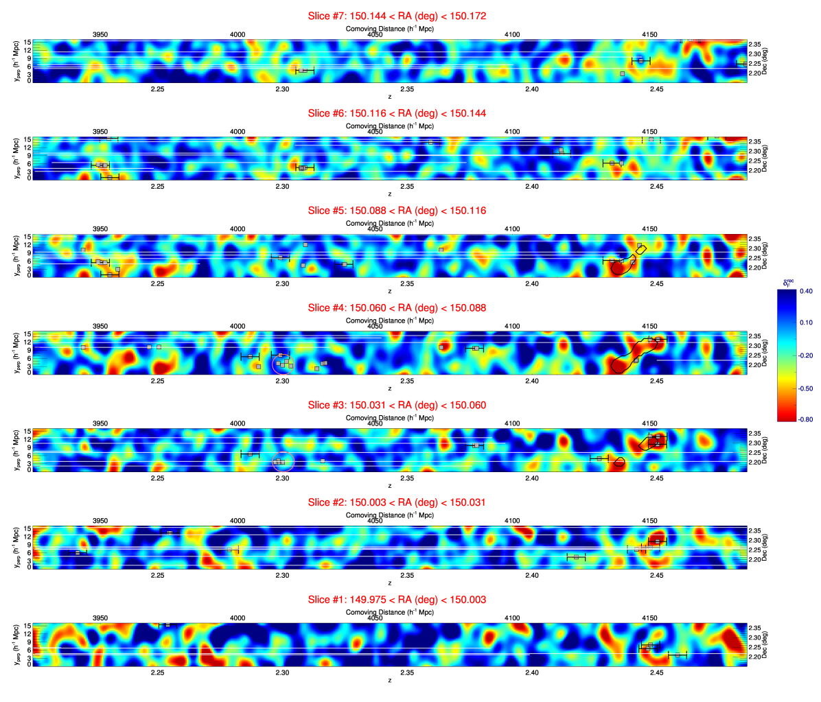
Figure 4.— Projections of our Ly$\alpha$ forest tomographic map across $2h^{-1}{\rm\ Mpc}$ slices in the R.A. direction, with the slice locations indicated in Figure 2. Note that negative values of $\delta_{F}^{\rm rec}$ (red colors) correspond to higher overdensities, while the white horizontal lines represent the skewer sampling from the background sources. Grey squares mark the positions of coeval galaxies with spectroscopic redshifts from the zCOSMOS (Lilly et al., 2007) and MOSDEF (K15) surveys. The error bars indicate the LOS uncertainties associated with LBG redshift determination, while the galaxies without error bars have NIR redshifts, in which case the symbol widths denote the LOS uncertainty. Black contours in Slices #3-5 (at $z\approx 2.435-2.450$) delineate regions with $\delta_{F}^{\rm sm}<-3.5\,\sigma_{\rm sm}$, which is the protocluster criterion defined by S15. Pink circles in Slices #3-4 indicate the $z=2.300$ compact overdensity of MOSDEF galaxies within our volume.

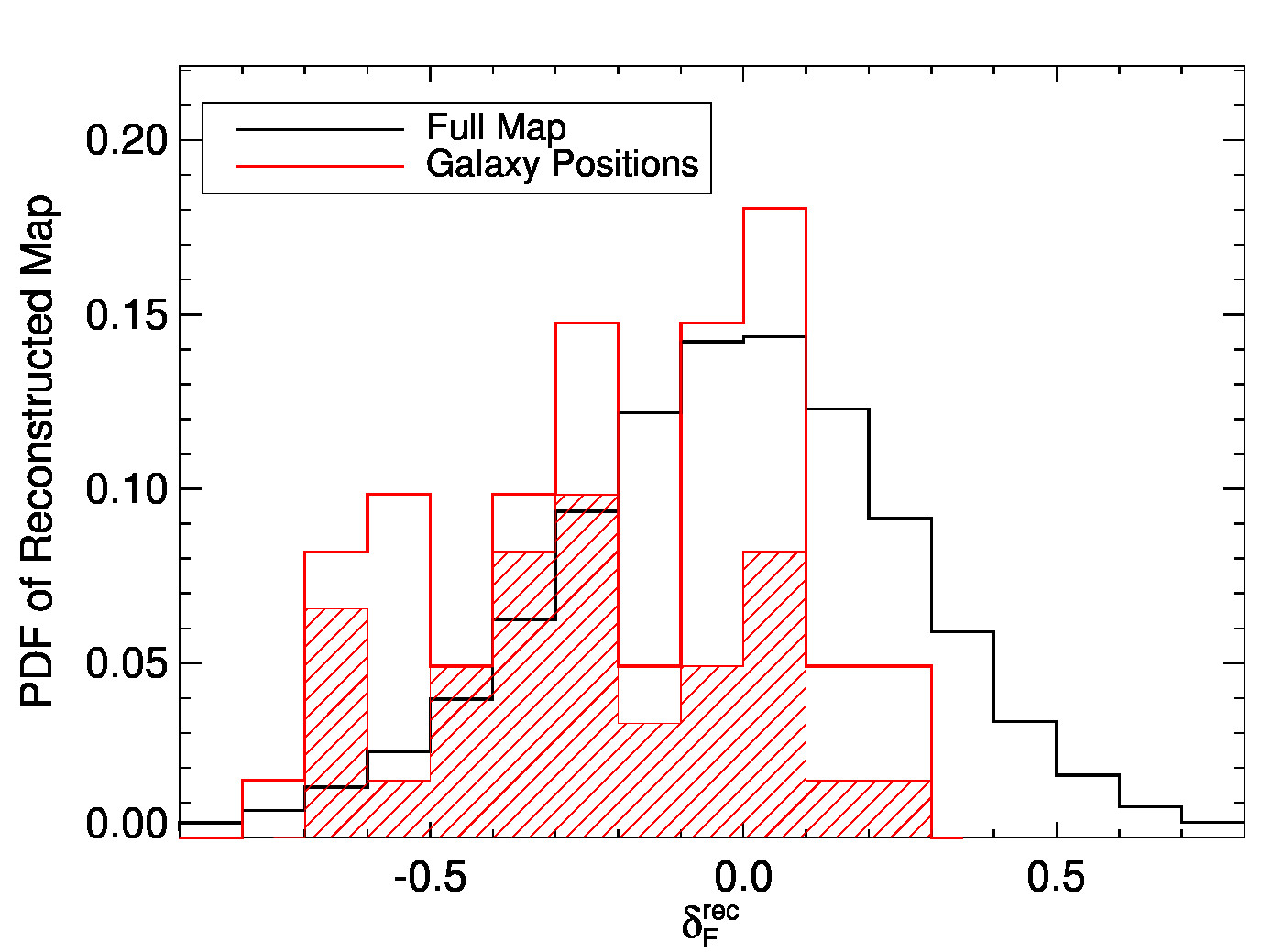
Figure 5.— PDF of the reconstructed absorption from our map (black), along with the corresponding PDF at the position of the 61 coeval galaxies (red); negative absorption corresponds to higher overdensities. The galaxies PDF is clearly skewed towards overdense regions of the map; this is even clearer in the case of the subsample of 31 MOSDEF redshifts (shaded red histogram).

The resulting tomographic reconstruction of the foreground IGM is presented in Figure 3 as a 3D visualization, while Figure 4 shows the same map as a series of 2D projections across $\Delta\chi=2\,h^{-1}{\rm\ Mpc}$ along the R.A. direction; a movie of the 3D visualization can be viewed online. As in L14b, we see large overdensities and underdensities spanning $\gtrsim 10\,h^{-1}{\rm\ Mpc}$. The enlarged map volume also allows us to repeat the comparison of the map with coeval galaxies within the same volume. Using an internal compilation of spectroscopic redshifts within the COSMOS field (albeit updated from the one used in L14b), we find 61 coeval galaxies, primarily from the zCOSMOS-Deep (Lilly et al., 2007), VUDS (Le Fèvre et al., 2015) and MOSDEF (K15) surveys. We overplot these galaxy positions on Figure 4. These aforementioned surveys are known to be uniformly flux-limited; we momentarily leave out galaxies targeted specifically as protocluster members, which will be discussed in Section 5.

We compare the distribution of map values at the galaxy positions with the overall map PDF in Figure 5. There is a clear skew in the absorption at the galaxies’ positions towards negative $\delta_{F}^{\rm rec}$ values, confirming that both the tomographic map and galaxy positions sample high-density regions. A two-sample Kolgomorov-Smirnov test finds $P=5.7\times 10^{-5}$ that the galaxy values are drawn from the overall distribution; this is a considerable improvement from the analogous comparison with 18 coeval galaxies in L14b, which had $P=0.24$.

There are several effects, however, that can introduce scatter into this comparison between galaxy positions and the large-scale IGM. Even in the absence of map reconstruction errors and with perfect redshift determinations, one expects a slight mismatch from the slightly different velocity fields traced by galaxies and the Ly$\alpha$ forest, which is in turn due to the different halo biases of both tracers. However, in our case we expect the primary sources of scatter to be reconstruction errors in the tomographic map, as well as line-of-sight positional uncertainties ($\sigma_{v}\sim 300\,~{}{\rm km~{}s}^{-1}$ or $\sigma_{\mathrm{los}}\sim 3.5\,h^{-1}{\rm\ Mpc}$) on the galaxies comparable to our map resolution. The latter arises from redshift errors induced by low spectral resolution ($R<200$) (Lilly et al., 2007; Le Fèvre et al., 2013) as well as intrinsic scatter between the true systemic redshift compared with redshift estimates from Ly$\alpha$ emission or UV absorption lines (e.g. Adelberger et al., 2005; Steidel et al., 2010; Rakic et al., 2011). L14b showed using simulated reconstructions that this redshift error, along with reconstruction noise in the tomographic maps, would scatter some galaxies from overdensities into adjacent underdensities in the tomographic map.

However, galaxy redshifts measured in the NIR have much smaller redshift errors ($\sigma_{v}\sim 60\,~{}{\rm km~{}s}^{-1}$, Steidel et al., 2010) due both to the higher resolution ($R\sim 3500$, Kriek et al., 2015) and the fact that rest-frame optical nebular lines are much better tracers of the systemic frame, so when we restrict the PDF comparison only to the 31 galaxies observed in the NIR by MOSDEF, we find an even stronger skew towards higher map overdensities: the MOSDEF galaxies sample a median map value of $\delta_{F}^{\rm rec}\approx-0.24$, whereas the other galaxies have a median of $\delta_{F}^{\rm rec}\approx-0.09$. This comparison is encouraging and indicates that with expanded map volumes, we will be able to study correspondingly larger samples of coeval galaxies as a function of large-scale environment, with cuts in various galaxy properties such as star-formation rates, metallicities, AGN activity etc.

It is worth briefly mentioning the large regions in our tomographic map with positive $\delta_{F}^{\rm rec}$ (blue regions in Figure 4) that are completely empty of galaxies. These likely correspond to the high-redshift voids recently discussed in Stark et al. (2015a), but we defer a more detailed investigation to a subsequent paper.

4. Simulations

Before we proceed to search for overdensities in the COSMOS tomographic map, we first describe the N-body simulations that we will use to facillitate our subsequent analysis, which are the same simulations as S15. These are $2560^{3}$-particle TreePM (White, 2002) simulations with $8.6\times 10^{7}\,h^{-1}M_{\odot}$ equal-mass particles within a $(256\,h^{-1}{\rm\ Mpc})^{3}$ comoving volume. The assumed cosmology was consistent with Planck Collaboration et al. (2013): $\Omega_{\rm m}\approx 0.31$, $\Omega_{\rm b}h^{2}\approx 0.022$, $h=0.6777$, $n_{s}=0.9611$, and $\sigma_{8}=0.83$.

Using a friends-of-friends algorithm to identify halos, S15 found 425 halos at $z=0$ with $M\geq 10^{14}\,h^{-1}{\rm\ Mpc}$ that were defined as galaxy clusters. The progenitor halos for each cluster were traced backwards to $z=2.5$, and their center-of-mass at that epoch defined as the corresponding $z=2.5$ protocluster positions.

The velocities and particles at $z=2.5$ were used to generate Ly$\alpha$ forest spectra with the fluctuating Gunn-Peterson approximation (Croft et al., 1998; Rorai et al., 2013). From these skewers, S15 also generated tomographic maps from realistic mock data sets with various sightline sampling and noise properties. These reconstructions used the same Wiener-filtering code described in Section 3. In this paper, we will work primarily with their simulated reconstructions with average sightline separation $\langle d_{\perp}\rangle=2.5\,h^{-1}{\rm\ Mpc}$ binned on to a $(1\,h^{-1}{\rm\ Mpc})^{3}$ grid, which were designed specifically to match the L14b data set, including the spectral resolution and $\mathrm{S/N}$ distribution in the mock spectra.

Since progenitors of massive $z\sim 0$ clusters occupy overdensities on $\sim 5-10\,h^{-1}{\rm\ Mpc}$ scales at $z>2$ (Chiang et al., 2013), S15 argued that an efficient way to identify $z\sim 2.5$ protoclusters in Ly$\alpha$ forest tomographic maps is to first smooth the map with a $\sigma=4\,h^{-1}{\rm\ Mpc}$ Gaussian kernel to obtain the smoothed flux $\delta_{F}^{\rm sm}$, and then identify regions with $\delta_{F}^{\rm sm}<-3.5\,\sigma_{\rm sm}$, where $\sigma_{\rm sm}^{2}$ is the map variance in the respective map after smoothing. We find $\sigma_{\rm sm}^{2}=3.5\times 10^{-3}$ in our real map, and $\sigma_{\rm sm}^{2}=3.8\times 10^{-3}$ the simulated maps.

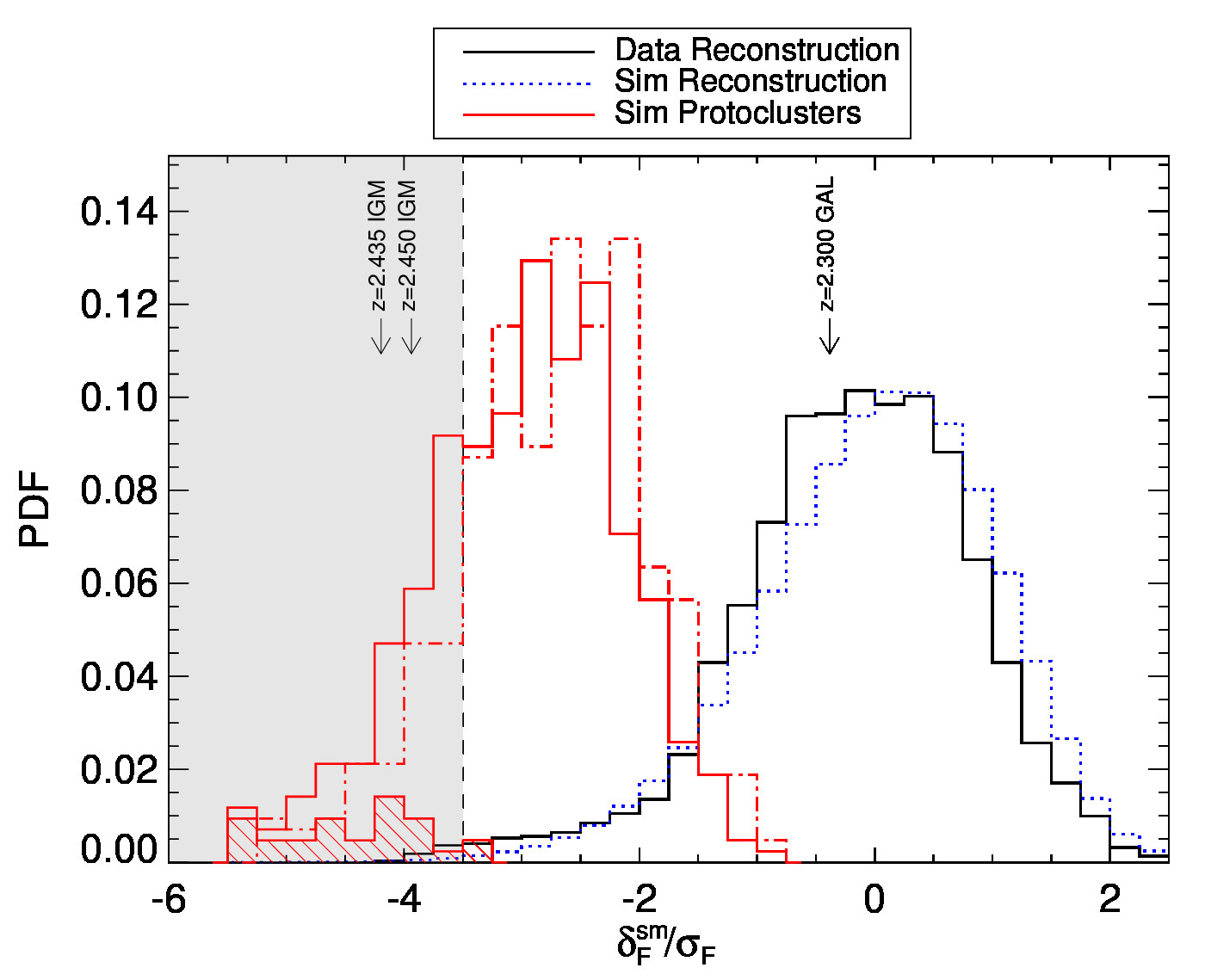
Figure 6.— PDF of the quantity $\delta_{F}^{\rm sm}/\sigma_{\rm sm}$ used to select for protoclusters. The black histogram shows the distribution from our real map, while the blue-dotted histogram shows that from simulated reconstructions. The distribution corresponding to the 425 $M(z=0)>10^{14}\,M_{\odot}$ protoclusters within the simulation is shown by the red histogram, while the hashed red histogram shows the subset of 27 protoclusters with $M(z=0)>5\times 10^{14}\,M_{\odot}$. The dotted-dashed red histogram shows the protocluster distribution including our toy feedback model (see Section 5.2). The shaded grey region indicates the $\delta_{F}^{\rm sm}/\sigma_{\rm sm}<-3.5$ criterion for selecting protoclusters. Downward arrows indicate the values corresponding to the $z=2.435$ and $z=2.450$ lobes of protocluster candidate found in our tomographic map, as well as the $z=2.300$ overdensity of MOSDEF galaxies.

\begin{overpic}[width=346.89731pt]{slice_xy_realizations_cl5000482.jpg} \put(-6.0,12.0){\rotatebox{90.0}{\color[rgb]{1,0,0} \scriptsize$M(z=0)=10^{15.0}\,h^{-1}{\rm\ M}_{\odot}$}} \end{overpic}

\begin{overpic}[width=346.89731pt]{slice_xy_realizations_cl3233112.jpg} \put(-6.0,12.0){\rotatebox{90.0}{\color[rgb]{1,0,0} \scriptsize$M(z=0)=10^{14.9}\,h^{-1}{\rm\ M}_{\odot}$}} \end{overpic}

\begin{overpic}[width=346.89731pt]{slice_xy_realizations_cl4831963.jpg} \put(-6.0,12.0){\rotatebox{90.0}{\color[rgb]{1,0,0} \scriptsize$M(z=0)=10^{14.1}\,h^{-1}{\rm\ M}_{\odot}$}} \end{overpic}

Figure 7.— Simulated $z=2.5$ galaxy protoclusters shown as projections on the sky plane with thickness $5\,h^{-1}{\rm\ Mpc}$ along the line-of-sight. Each map is centered on the center-of-mass of progenitor halos that will eventually collapse into $z=0$ clusters with (top to bottom) $M=[1.1\times 10^{15},8.8\times 10^{14},1.2\times 10^{14}]\,h^{-1}{\rm\ M}_{\odot}$. The left panel on each row shows the underlying DM distribution (smoothed on $1\,h^{-1}{\rm\ Mpc}$ scales), while the other three panels show tomographic reconstructions from different realizations of mock Ly$\alpha$ forest data with similar sightline separations ($\langle d_{\perp}\rangle=2.5\,h^{-1}{\rm\ Mpc}$) and noise as our data. The black contours overplotted on the tomographic maps indicate regions that satisfy our protocluster criterion of $\delta_{F}^{\rm sm}<-3.5\,\sigma_{\rm sm}$ after smoothing. While this threshold robustly selects massive cluster progenitors, it is marginal for lower-mass protoclusters such as the bottom panel. Note that in the middle panel, the lobe to the upper left ($[\Delta x,\Delta y]\approx[-10,8]\,h^{-1}{\rm\ Mpc}$) will in fact a collapse into a separate, albeit lower mass ($M=1.5\times 10^{14}\,h^{-1}{\rm\ M}_{\odot}$) $z\sim 0$ cluster than the central object.

In Figure 6 we show the distribution of smoothed $\delta_{F}^{\rm sm}/\sigma_{\rm sm}$ values from the overall $(256\,h^{-1}{\rm\ Mpc})^{3}$ simulation volume (dotted-blue histogram), while the red histogram shows the minimum $\delta_{F}^{\rm sm}/\sigma_{\rm sm}$ within $4\,h^{-1}{\rm\ Mpc}$ of each of the 425 protoclusters within the simulation; the shaded histogram shows the subset of 27 protoclusters that will grow into $M>5\times 10^{14}\,h^{-1}{\rm\ Mpc}$ clusters by $z=0$. This clearly shows that protoclusters occupy extreme $\delta_{F}^{\rm sm}/\sigma_{\rm sm}$ regions that are well-separated from the overall distribution.

S15 have shown that this method of selecting protoclusters yields good purity: applying the same selection criteria on the simulated tomographic map with $\langle d_{\perp}\rangle=2.5\,h^{-1}{\rm\ Mpc}$, we found 89 candidate protoclusters of which 81 will eventually collapse into a $M\geq 10^{14}\,h^{-1}\,h^{-1}{\rm\ M}_{\odot}$ halo by $z=0$ ($\sim 90\%$ purity); another 7 candidates ($\sim 8\%$) have group-sized descendants of $3\times 10^{13}\,h^{-1}{\rm\ M}_{\odot}<M(z=0)<10^{14}\,h^{-1}{\rm\ M}_{\odot}$, while only 1 candidate ($\sim 1\%$) will evolve into a low-mass halo ($M(z=0)<3\times 10^{13}\,h^{-1}{\rm\ M}_{\odot}$). These results are qualitatively similar to those found by S15 but are not numerically identical despite being applied to the same simulations; this is likely because we have slightly different linking criteria for identifying contiguous thresholded regions.

Figure 7 shows several of the simulated protoclusters, in each case comparing three tomographic reconstructions matched to the L14b data, but with different random realizations of the sightline positions and pixel noise. The progenitors of massive clusters occupy such extended overdensities that they can be robustly detected with our sightline sampling, although at lower masses ($M(z=0)\sim 10^{14}\,h^{-1}{\rm\ M}_{\odot}$) the absorption signature can be less pronounced and is less likely to be selected by our criterion (e.g. bottom panel of Figure 7).

The overall completeness of the S15 selection criterion is $\sim 20\%$ for all $M(z=0)>10^{14}$ cluster progenitors (81/425), but this improves dramatically for higher-mass progenitors: we detect 41/51 protoclusters with $M(z=0)>3\times 10^{14}\,h^{-1}{\rm\ M}_{\odot}$ ($\sim 80\%$ completeness) and 24/27 protoclusters with $M(z=0)>5\times 10^{14}\,h^{-1}{\rm\ M}_{\odot}$ ($\sim 90\%$ completeness). The comoving space density of $M(z=0)>10^{14}\,h^{-1}{\rm\ M}_{\odot}$ clusters is $n\approx 2.5\times 10^{-5}\,h^{3}\,\mathrm{Mpc}^{-3}$ within our simulation, which translates to an expectation of $\sim 1.5$ protoclusters within our present observed map volume ($V\approx 5.8\times 10^{4}\,h^{-1}{\rm\ Mpc}$).

Figure 6 also shows the smoothed $\delta_{F}^{\rm sm}/\sigma_{\rm sm}$ distribution from our COSMOS tomographic map (black histogram), with both the $\sigma_{\rm sm}$ values derived individually for the data and simulated maps. There is some disagreement in the distributions from the data and the simulations, but the Ly$\alpha$ forest absorption PDF is known to be a notoriously difficult quantity to model: our simulation used a DM-only N-body code that models only gravitational clustering, but not the hydrodynamics of the IGM (White et al., 2010), nor have we attempted to accurately model systematics such as the continuum-errors, spectral noise, optically-thick absorbers (e.g., Lee et al., 2015), temperature-density relationship, or Jeans smoothing (Rorai et al., 2013). For the present analysis, it is of some concern that our map PDF is somewhat larger at $\delta_{F}^{\rm sm}<-3.5\,\sigma_{\rm sm}$ than the simulated PDF, but this is likely to be due to damped Ly$\alpha$ absorbers (DLAs) and Lyman-limit systems (LLS’s) with column densities of $N_{\mathrm{HI}}\gtrsim 10^{17}\,\,\mathrm{cm^{-2}}$ contaminating individual sightlines. By adding individual fake DLAs to our simulated reconstructions, we found that these could cause small regions with limited transverse extent ($\lesssim 1\,h^{-1}{\rm\ Mpc}$) to cross our protocluster threshold, but they cannot cause extended transverse IGM signatures characteristic of massive protoclusters (Figure 7), since this requires strong correlated absorption across multiple adjacent sightlines. Over the total $\Delta z\sim 12$ redshift path-length of our Ly$\alpha$ forest spectra we expect only $\sim 2$ DLAs with $N_{\mathrm{HI}}>10^{20.3}\,\,\mathrm{cm^{-2}}$ (Prochaska et al., 2005), which makes it very unlikely that chance alignments of DLAs could cause a spurious protocluster candidate. Careful forward-modeling of such systematics would be desirable to characterize marginal protocluster candidates in future data sets, but as we shall see we have only one protocluster candidate in our data, which is highly extended ($\gtrsim 10\,h^{-1}{\rm\ Mpc}$) in both the transverse and line-of-sight dimensions.

S15 showed that various quantities related to the Ly$\alpha$ forest absorption signature of simulated $z=2.5$ protoclusters can be related to their $z=0$ descendant masses, although they showed this mostly as a function of the ‘true’ Ly$\alpha$ absorption field in the simulation. We now carry out a similar analysis, but incorporating forward modeling by using the 81 protoclusters identified through the tomographic maps of the same simulated absorption field, which incorporate realistic random sparse sampling of the intervening sightlines as well as noise and spectral resolution matched to our data. This can then be directly compared with overdensities identified in our data (Section 5.1). In the following discussion, ‘protocluster candidates’ refer to $\delta_{F}^{\rm sm}<-3.5\,\sigma_{\rm sm}$ regions in the $\sigma=4\,h^{-1}{\rm\ Mpc}$ Gaussian-smoothed tomographic maps. Individual protocluster candidates are defined through a $4\,h^{-1}{\rm\ Mpc}$ linking length regardless of physical continuity, so it is possible for a single candidate to be comprised of multiple disconnected structures, so long as their voxels can be linked to within $4\,h^{-1}{\rm\ Mpc}$.

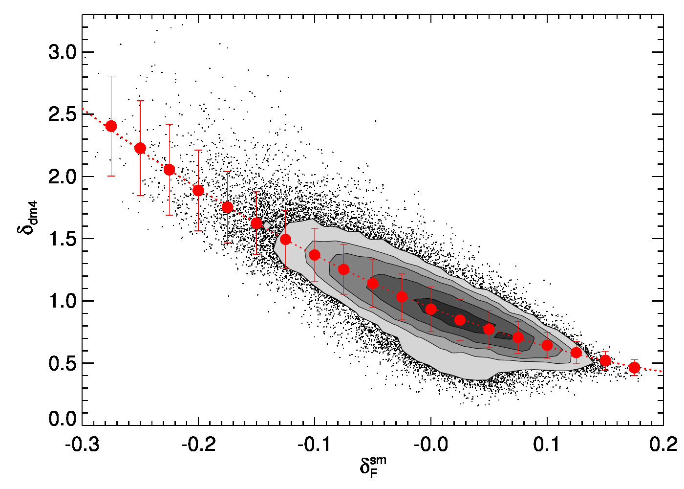
Figure 8.— Scatter-plot of the smoothed Ly$\alpha$ forest tomographic map flux in our simulation against underlying DM overdensity smoothed on the same $4\,h^{-1}{\rm\ Mpc}$ scale, evaluated in $(1\,h^{-1}{\rm\ Mpc})^{3}$ map voxels. The contours denote the 10th, 20th, 30th, 50th and 80th percentiles of the distribution, while the red circles denote the means within bins of $\Delta\delta_{F}^{\rm sm}=0.02$ along with the standard deviations as error bars. The red-dotted line shows the 2nd-order polynomial fitted to the distribution (Eq. 4).

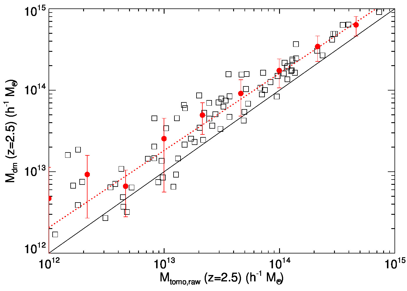
Figure 9.— Tomographic mass of protocluster candidates in our simulation, compared with the true DM mass within each protocluster region at the same redshift of $z=2.5$. The solid black line shows the 1:1 linear slope, while the dotted red line shows the best-fit power-law fit to correct the tomographic masses (Eq. 6).

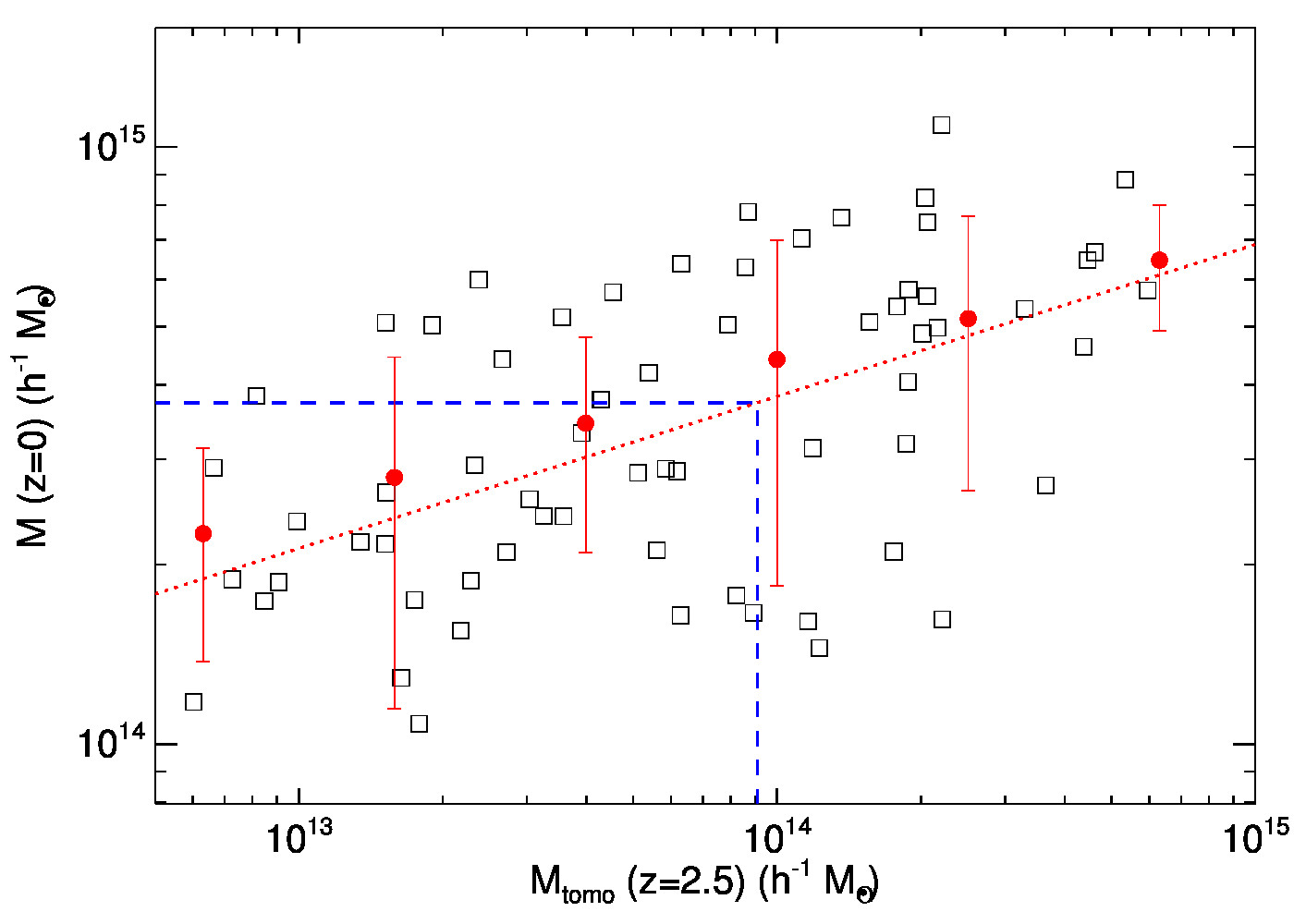
Figure 10.— Descendant cluster mass at $z=0$, as a function of the corrected tomographic mass (Eq. 6) in $z=2.5$ protoclusters detected in simulated tomographic maps. Red points show the mean and standard deviation in logarithmic bins of $0.4\,$dex in $M_{\rm tomo}$, while the dotted red line shows the best-fit power-law through the points (Eq. 7). The blue dashed line indicates the value corresponding to our observed $z\approx 2.45$ IGM overdensity (Sec. 5.1).

Since the Ly$\alpha$ forest absorption is a tracer of the underlying dark matter (DM) density, it should be possible to estimate the total $z\sim 2.5$ mass encompassed by IGM protocluster candidates. While a full inversion of the underlying matter density field from IGM tomographic maps is a challenging problem beyond the scope of this work (although see Nusser & Haehnelt, 1999; Pichon et al., 2001; Kitaura et al., 2012), we can use our simulations for the more limited goal of estimating the $z=2.5$ mass enclosed within the protocluster regions. This exploits the tight relationship found by Lee et al. (2014a) between the map flux after smoothing by $\sigma=4\,h^{-1}{\rm\ Mpc}$ Gaussian, $\delta_{F}^{\rm sm}$, and $\delta_{\mathrm{dm4}}$, the underlying DM overdensity smoothed to the same scale. Figure 8 shows this relationship from our simulation (binned in $(1\,h^{-1}{\rm\ Mpc})^{3}$ voxels), which can be fitted with a 2nd-order polynomial:

$$\delta_{\mathrm{dm4}}\approx 5.502\,(\delta_{F}^{\rm sm})^{2}-3.681\,\delta_{F}^{\rm sm}+0.947.$$ (4)

We then apply this mapping to the $\delta_{F}^{\rm sm}$ values within $z=2.5$ tomographic map voxels encompassed by the $\delta_{F}^{\rm sm}/\sigma_{\rm sm}<-3.5$ protocluster contour, and then sum these DM overdensities over the protocluster candidate (‘pc’) region to define a raw ‘tomographic mass’:

$$M_{\rm tomo,raw}=\left(\sum^{\rm pc}\delta_{\mathrm{dm4}}\right)\times\;8.1\times 10^{10}h^{-1}{\rm\ M}_{\odot},$$ (5)

where $M=8.1\times 10^{10}h^{-1}{\rm\ M}_{\odot}$ is the cosmic mean density of DM and baryons multiplied by the $(1\,h^{-1}{\rm\ Mpc})^{3}$ comoving volume of our map voxels. Figure 9 shows the estimated $z=2.5$ raw tomographic masses for the protocluster candidates in our simulation against the ‘true’ unsmoothed DM mass within each protocluster region. There is a reasonably tight relationship between $M_{\rm dm}$ and $M_{\rm tomo,raw}$, but the latter systematically underestimates by $\sim 20-30\%$ the true DM mass over the $\sim 10^{13-14}\,h^{-1}{\rm\ M}_{\odot}$ range typical of our protocluster regions, because it was calibrated to the smoothed DM field and not the true DM field (binned in $(1\,h^{-1}{\rm\ Mpc})^{3}$ cells in our simulation). Since the protocluster boundaries (defined by $\delta_{F}^{\rm sm}/\sigma_{\rm sm}<-3.5$) are still significantly overdense, the smoothing smears DM out of the protocluster regions hence causing an underestimate of protocluster mass. To get an accurate estimate of the $z=2.5$ DM mass enclosed within any protocluster candidates identified in a tomographic map, we would therefore need to correct the raw tomographic masses by the power-law found to fit Figure 9:

$$M_{\rm tomo}\approx 10^{14.21}\left(\frac{M_{\rm tomo,raw}}{10^{14}\,h^{-1}{\rm\ M}_{\odot}}\right)^{0.946}\,h^{-1}{\rm\ M}_{\odot}.$$ (6)

This is the formula we use when we henceforth refer to ‘tomographic masses’. Since this calibration is based on tomographic maps with realistic sightline sampling and noise, the scatter in Figure 9 provides a measure of the uncertainty in the protocluster mass estimate: for example, the uncertainty in the mass estimate for a $M_{\rm tomo}(z=2.5)=10^{14}\,h^{-1}{\rm\ M}_{\odot}$ protocluster is $\sigma_{\rm tomo}\approx 5\times 10^{13}\,h^{-1}{\rm\ M}_{\odot}$.

As suggested by S15, we also checked if the $z=2.5$ tomographic protocluster mass could be used to predict the $z=0$ descendant mass. This is shown for our simulated protocluster candidates in Figure 10, where we see a trend for increasing $M(z=0)$ with $M_{\rm tomo}$, which can be fitted with the following power-law:

$$M(z=0)\approx 10^{14.5}\left(\frac{M_{\rm tomo}}{10^{14}\,h^{-1}{\rm\ M}_{\odot}}\right)^{0.25}\,h^{-1}{\rm\ M}_{\odot}.$$ (7)

Part of the $\sim 0.2\,$dex scatter in this relationship is due to the reconstruction error in our simulated tomographic maps (since we have realistic pixel noise and sightline sampling), but S15 have also shown that the dominant contributor to this scatter is in fact intrinsic, i.e. due to diversity in the morphologies of cluster progenitors at fixed $M(z=0)$.

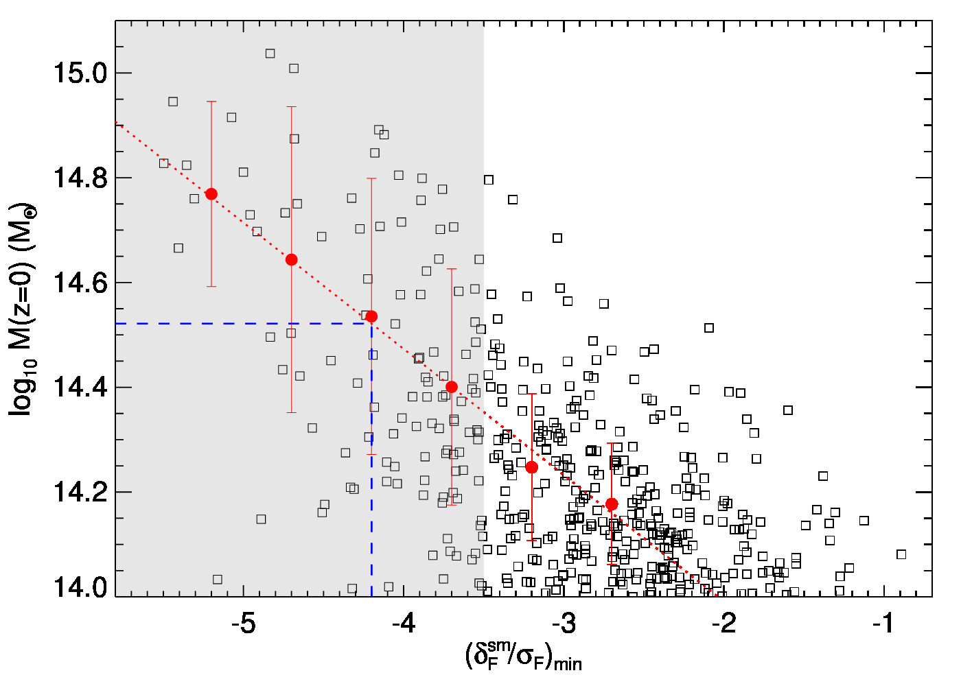
Figure 11.— Relationship between the smoothed absorption peak associated with all $z=2.5$ protoclusters in our simulated tomographic map, and the final $z=0$ cluster mass. The red points with error bars show the average $M(z=0)$ in bins of $\Delta(\delta_{F}^{\rm sm}/\sigma_{\rm sm})_{\rm min}=0.5$ and the associated standard deviations, while the dotted-blue line is the relationship fitted to the distribution (Eq. 8). The shaded gray region is our $\delta_{F}^{\rm sm}/\sigma_{\rm sm}<-3.5$ criterion used for protocluster selection in the tomographic maps. Blue dashed lines indicate the value corresponding to the observed $z\approx 2.45$ IGM overdensity in our map (Sec. 5.1).

Another quantity shown by S15 to correlate with $z=0$ cluster mass is the IGM absorption peak associated with the protocluster candidates in the smoothed tomographic maps. Figure 11 shows this for our simulated protocluster candidates. Again, we see a relationship between the absorption depth $(\delta_{F}^{\rm sm}/\sigma_{\rm sm})_{\rm min}$ and the final $z=0$ cluster mass, although there is more scatter than the analogous plot in S15 (Figure 5 in their paper) since we are working with realistic reconstructed tomographic maps rather than the ‘true’ absorption field in the simulation. We fit the following function to the distribution:

$$M(z=0)\approx 10^{13.5-0.24\,(\delta_{F}^{\rm sm}/\sigma_{\rm sm})_{\mathrm{min}}}\,h^{-1}{\rm\ M}_{\odot}.$$ (8)

This absorption depth provides an alternative to $M_{\rm tomo}$ as an estimator for $M(z=0)$, although both quantities are not completely independent.

5. Map Overdensities

In this section, we analyze our reconstructed Ly$\alpha$ forest map (Section 3) and look for IGM overdensities, aided by what we learned from the analysis of simulations in the previous section. We will then also discuss two overdensities within our volume identified from external galaxy datasets.

5.1. IGM Overdensities

5.1.1 $z=2.45$ Protocluster

We now apply the S15 protocluster criterion on our COSMOS tomographic map. After smoothing by a $\sigma=4\,h^{-1}{\rm\ Mpc}$ Gaussian kernel, we find one large IGM overdensity within our map that clearly satisfies the $\delta_{F}^{\rm sm}<-3.5\,\sigma_{\rm sm}$ protocluster threshold (Figure 4). The absorption peak is at a redshift of $z=2.450$ and approximately centered on [RA, Dec]$\approx[150.06,2.31]\,$deg, although there is a secondary peak at $z=2.435$ within contour defined by the $\delta_{F}^{\rm sm}<-3.5\,\sigma_{\rm sm}$ threshold; these two peaks have smoothed absorption values of $\delta_{F}^{\rm sm}=[-3.9,-4.2]$ at $z=[2.435,2.450]$, respectively, which are also marked in Figure 6. This overdensity is highly extended in both the line-of-sight and transverse dimensions: it can be seen in Figure 4 to continuously extend from $z\approx 2.435-2.450$ (Slices #3-5), while Figure 12 shows line-of-sight map projections centered on the two absorption peaks of this overdensity ($z=2.435$ and $z=2.450$), showing that it spans up to $\sim 10\,h^{-1}{\rm\ Mpc}$ ($\sim 4\,$pMpc) in the transverse direction — the overall morphology of the protocluster in the unsmoothed map can be seen in Figure 13. The total comoving volume of this protocluster candidate (defined as that within the $\delta_{F}^{\rm sm}<-3.5\,\sigma_{\rm sm}$ contour) is $V\approx 340\,h^{-3}\,\mathrm{Mpc}^{3}\approx(7\,h^{-1}{\rm\ Mpc})^{3}$. Assuming pure Hubble flow, we evaluate the pairwise separations between all voxels within the overdensity to find a maximum linear extent of $L_{\rm max}\approx 19\,h^{-1}{\rm\ Mpc}$, which subtends over twice our effective spatial resolution element (defined as $2.3\times$ our effective reconstruction length of $3.5\,h^{-1}{\rm\ Mpc}$). Applying the ‘tomographic mass’ estimation calibrated with our simulations (Equations 4, 5, and 6), the total DM mass enclosed within the $\delta_{F}^{\rm sm}/\sigma_{\rm sm}<-3.5$ contour is $M_{\rm dm}\equiv M_{\rm tomo}=(9\pm 4)\times 10^{13}\,h^{-1}{\rm\ M}_{\odot}$, where the uncertainty is estimated from the scatter seen in the simulated protoclusters (Figure 9).

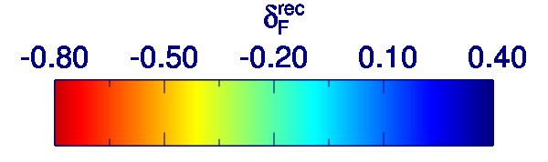
\begin{overpic}[width=186.45341pt,clip={true},trim=0.0pt 24.09pt 0.0pt 0.0pt]{pcslice_xy_z2430-2440.jpg} \put(42.0,233.0){{(a)}} \end{overpic}

\begin{overpic}[width=186.45341pt,clip={true},trim=0.0pt 24.09pt 0.0pt 0.0pt]{pcslice_xy_z2445-2455.jpg} \put(42.0,233.0){{(b)}} \end{overpic}

Figure 12.— Projections of our tomographic map along the line-of-sight, centered on two lobes of the large IGM overdensity identified through the $\delta_{F}^{\rm sm}<-3.5\,\sigma_{\rm sm}$ protocluster-finding threshold advocated by S15. The projected redshift range and line-of-sight thickness is labeled above each panel, and were chosen to incorporate a reasonable number of coeval galaxies within the projection. Open circles mark the sightlines sampling each projected slice, while filled symbols indicate coeval galaxies within the map: MOSDEF galaxies (inverted triangles, K15); zCOSMOS-Deep LBGs (stars, Lilly et al., 2007); LAEs from C15 (triangles); and LBGs from D15 (squares). The black contour denotes the region that satisfies our protocluster criterion of $\delta_{F}^{\rm sm}/\sigma_{\rm sm}<-3.5$ after smoothing.

\begin{overpic}[width=212.47617pt]{pilot2_3d_pc.jpg} \put(112.0,134.0){\vector(1,-3){14.0}} \put(91.0,137.0){\footnotesize$\mathsf{z=2.450}$} \put(180.0,110.0){\vector(1,-1){25.0}} \put(160.0,115.0){\footnotesize$\mathsf{z=2.480}$} \put(58.0,52.0){\vector(4,3){39.0}} \put(35.0,43.0){\footnotesize$\mathsf{z=2.435}$} \end{overpic}

Figure 13.— Still frame from the video in Fig. 3 centered on the IGM overdensity at $z\approx 2.44$, with the line-of-sight distance ($z$-axis) increasing towards the right. Arrows indicate the two absorption peaks ($z=2.435$ and $z=2.450$) associated with the $z\approx 2.45$ protocluster, as well as the $z=2.48$ protocluster from Casey et al. (2015) at the edge of our map (Section 5.2).

This IGM overdensity corresponds to a known object: D15 recently reported a $z=2.450$ protocluster comprising of 11 LBGs, several of which we plot as filled squares in Figure 12. This protocluster was corroborated by a more recent spectroscopic study of Ly$\alpha$ emitters (LAEs) by C15, which are plotted as filled triangles in Figure 12. The position of these LBGs and LAEs at $z\approx 2.435-2.450$ appear spatially well-correlated with our Ly$\alpha$ overdensity at the same redshifts. The tomography also shows that the elongated transverse configuration of the $z=2.450$ protocluster galaxies is due to two sub-structures at that redshift (Figure 12a) connected by a lower-density ‘bridge’ well-sampled by our sightlines. Note that due to edge effects, it is possible that the protocluster might extend beyond our map boundary. Figures 4 and 13 suggest that there could be a bridging filament between the $z=2.435$ and $z=2.450$ lobes of the overdensity, although deeper observations with better sightline sampling and better spectral $\mathrm{S/N}$ would be required to verify this.

We now make an estimate of the descendant ($z=0$) mass of this protocluster based on its IGM tomography signature at $z=2.45$. The $z=2.45$ tomographic mass enclosed within its $\delta_{F}^{\rm sm}/\sigma_{\rm sm}<-3.5$ boundaries implies, through Equation 7, that it will eventually collapse into a $M(z=0)=(3.1\pm 2.5)\times 10^{14}\,h^{-1}{\rm\ M}_{\odot}$ object, i.e. an intermediate-mass Virgo-like cluster. The uncertainty is, again, based on the scatter of in the simulated protoclusters (Figure 10 with which we calibrated Equation 7. The maximum smoothed absorption associated with the protocluster also provides an alternative estimate of the $z\sim 0$ masses via Equation 8. Applied to the absorption peak of $(\delta_{F}^{\rm sm}/\sigma_{\rm sm})_{\mathrm{min}}\approx-4.2$ seen at $z=2.450$, this implies $z\sim 0$ masses of $M\approx(3.4\pm 2.1)\times 10^{14}\,h^{-1}{\rm\ M}_{\odot}$. While these two estimates are not fully independent since $M_{\rm tomo}$ is calibrated through the map pixel values, it is reassuring that they give similar values.

5.1.2 One or two $z=0$ clusters?

From the unsmoothed tomographic map (Figure 4 or 13), the $z=2.45$ IGM overdensity is comprised of two separate lobes at $z\approx 2.435$ and $z\approx 2.450$. After imposing the smoothed $\delta_{F}^{\rm sm}/\sigma_{\rm sm}<-3.5$ cut for protocluster selection, the resulting contour is continuous but still has two absorption peaks: the more significant one ($\delta_{F}^{\rm sm}/\sigma_{\rm sm}=-4.2$) at $z=2.450$ with the other at the $z=2.435$ lobe with $\delta_{F}^{\rm sm}/\sigma_{\rm sm}=-3.9$, with a comoving separation of $\approx 16\,h^{-1}{\rm\ Mpc}$ assuming only Hubble flow in the radial direction. Interestingly, if we split our evaluation of the underlying tomographic mass to either side of $z=2.442$ (the approximate saddle point between the two lobes) we find that the the $z=2.435$ part is actually slightly more massive at $M_{\rm tomo}\approx 5\times 10^{13}\,h^{-1}{\rm\ M}_{\odot}$ compared with $M_{\rm tomo}\approx 4\times 10^{13}\,h^{-1}{\rm\ M}_{\odot}$ at $z=2.450$. While this difference is insignificant compared to our uncertainties, it does point to the overdensity being comprised of two roughly equal-mass portions at $\sim 15\,h^{-1}{\rm\ Mpc}$ separation. One might then wonder whether this protocluster candidate will in fact collapse into a single $z\sim 0$ cluster, or two separate ones.

Figure 14.— The elongation of IGM protocluster candidates identified in the simulated tomographic maps. In the top panel, we show the descendant mass $M(z=0)$ associated with each protocluster candidate as a function of the elongation ratio $L_{\rm max}/V^{1/3}$. In the cases where there is a second cluster progenitor associated with the IGM candidate, the secondary protocluster is indicated with a blue circle and connected to the primary with a blue line. The middle panel shows the distribution of $L_{\rm max}/V^{1/3}$ with the subset of binaries in blue, while the bottom panel shows the binary fraction at each $L_{\rm max}/V^{1/3}$ bin. Vertical red dashed line indicates the value from the $z=2.45$ protocluster in our observed map.

To provide some insight, we again turn to the simulated protoclusters detected in tomography. S15 described such situations in the protocluster search process, in which a single $z=2.5$ IGM protocluster candidate is in fact associated with progenitors from two separate $z=0$ clusters. Out of the 81 protoclusters identified through our simulated $(256\,h^{-1}{\rm\ Mpc})^{3}$ tomographic map, we find that 21 ($\sim 25\%$) could in fact be associated with a secondary $z=0$ cluster. We noticed that many of these ‘binary’ protoclusters appeared elongated (e.g. middle panel in Figure 7), so we compute $L_{\rm max}/V^{1/3}$ on their $\delta_{F}^{\rm sm}/\sigma_{\rm sm}<-3.5$ boundaries as a rough measure of their elongation. This is shown in Figure 14, which compares $L_{\rm max}/V^{1/3}$ with $M(z=0)$ for both unitary and binary protoclusters. In the lower panels of Figure 14, we see that the binary fraction of the IGM protocluster candidates is low ($\sim 10\%$) for roughly spherical ($L_{\rm max}/V^{1/3}\sim 1$) overdensities but increases with $L_{\rm max}/V^{1/3}$ and approaches unity at $L_{\rm max}/V^{1/3}\sim 2.5$, i.e. protocluster candidates that appear highly elongated in the smoothed IGM tomographic maps are likely to evolve into two separate clusters by $z\sim 0$.

Our $z=2.45$ IGM overdensity has a maximum extent of $L_{\rm max}\approx 19\,h^{-1}{\rm\ Mpc}$ and an enclosed volume of $V\approx 340\,h^{-3}\,\mathrm{Mpc}^{3}$, which leads to $L_{\rm max}/V^{1/3}\sim 2.7$. This extreme value is only sampled by a handful of simulated protocluster candidates in Figure 14, but we see that $\sim 80\%$ of simulated protoclusters with $L/V^{1/3}>2$ collapsed into two separate $z=0$ clusters. This indicates a high probability that the IGM overdensity in our map will eventually collapse into two separate $z=0$ clusters with $M(z=0)\sim 10^{14}\,h^{-1}{\rm\ M}_{\odot}$, centered on the two absorption peaks at $z=2.435$ and $z=2.450$.

5.1.3 Less Significant IGM Overdensities

Apart from the significant $z=2.450$ IGM overdensity in our map that fulfils the protocluster criterion defined by S15, there are also several smaller ‘hot-spots’ that can be seen in the unsmoothed map (Figures 3 and 4), none of which fulfill the $\delta_{F}^{\rm sm}<-3.5\,\sigma_{\rm sm}$ threshold due to their limited size. In Slices #4-6, there are two smaller overdensities at $z\approx 2.23$ and $z\approx 2.25$ with transverse extents of $\lesssim 5\,h^{-1}{\rm\ Mpc}$ in the lower part of the map ($y_{\mathrm{perp}}\approx 6\,h^{-1}{\rm\ Mpc}$ and $y_{\mathrm{perp}}\approx 3\,h^{-1}{\rm\ Mpc}$, respectively). These overdensities have map values of $\delta_{F}^{\rm sm}\approx[-2.1,-1.8]\,\sigma_{\rm sm}$ after smoothing and thus do not satisfy our protocluster criterion, although there are several galaxies associated with a weaker extension of the $z\approx 2.23$ structure in Slices #5 and #6. There are another two apparent overdensities in Slice #1 at $z\approx 2.27$ and $z\approx 2.48$ at $y_{\mathrm{perp}}\approx 3\,h^{-1}{\rm\ Mpc}$ and $y_{\mathrm{perp}}\approx 9\,h^{-1}{\rm\ Mpc}$, respectively. Neither of these overdensities ($\delta_{F}^{\rm sm}\sim[-1.4,-1.8]\,\sigma_{\rm sm}$) satisfy our protocluster criterion, although this part of the map likely suffers from edge effects. A better characterization of these possible overdensities would require an extention of the map area beyond its current boundaries.

\begin{overpic}[width=186.45341pt,clip={true},trim=0.0pt 24.09pt 0.0pt 0.0pt]{pcslice_xy_z2296-2304.jpg} \put(42.0,233.0){{(a)}} \end{overpic}

\begin{overpic}[width=186.45341pt,clip={true},trim=0.0pt 24.09pt 0.0pt 0.0pt]{pcslice_xy_z2462-2478.jpg} \put(42.0,233.0){{(b)}} \end{overpic}

Figure 15.— Same as Fig. 12, but focused on two galaxy overdensities within our map. Panel (a) is focused on a compact overdensity of MOSDEF galaxies (upside-down triangles), while (b) shows our partial coverage of the $z\approx 2.47$ protocluster recently reported by Casey et al. (2015). Open circles indicate our sightline sampling, while filled symbols indicate coeval galaxies within the map: MOSDEF galaxies (inverted triangles, K15); zCOSMOS-Deep LBGs (stars, Lilly et al., 2007), and a DSFG (diamond, Casey et al., 2015).

5.2. Galaxy Overdensities

Apart from the overdensity in the Ly$\alpha$ absorption map, we now discuss two galaxy overdensities from external data sets.

5.2.1 $z=2.30$

During our comparison of the map overdensities and coeval galaxies, we noticed a compact overdensity of MOSDEF galaxies at $z\approx 2.30$ centered on [RA, Dec] = [150.06, 2.20]deg (pink circles in Slices #3-4 of Figure 4); the line-of-sight projection centered on this redshift is also shown in 15a). This is comprised of 6 galaxies within $\approx 2\,h^{-1}{\rm\ Mpc}$ (or $\approx 1\,$pMpc) on the sky, and a line-of-sight extent of $\Delta z\approx 0.006$ or $\Delta v\approx 560\,~{}{\rm km~{}s}^{-1}$, corresponding to $\approx 6\,h^{-1}{\rm\ Mpc}$ ($\approx 2.6$pMpc) assuming Hubble flow. If these galaxies fairly trace the underlying population, then within the subtended comoving volume the number density is $\rho_{\mathrm{gal}}\sim 0.3\,h^{3}\,\mathrm{Mpc}^{-3}$, which translates to an overdensity of $\rho_{\mathrm{gal}}/\langle\rho_{\mathrm{gal}}\rangle\sim 40$ relative to a mean number density of $\langle\rho_{\mathrm{gal}}\rangle\sim 7\times 10^{-3}\,h^{3}\,\mathrm{Mpc}^{-3}$, estimated from $2<z<3$ sources with $H\leq 24.5$ in the Santini et al. (2015) CANDELS/GOOD-S catalog (see Lee et al. 2013b for a similarly compact $z\sim 3.7$ overdensity). Within this structure, the quartet of galaxies at [RA, Dec] $\approx[150.058,2.200]$deg is even more compact: with a sky footprint of $\sim 0.17\mathrm{arcmin}^{2}$ and $\Delta z\approx 0.003$, this implies $\rho_{\mathrm{gal}}/\langle\rho_{\mathrm{gal}}\rangle\gtrsim 100$.

In Figures 4 and 15a, we do not see any large absorption decrement associated with these galaxies, although the sightline sampling could be better. These galaxies occupy map values of $\delta_{F}^{\rm rec}\sim-0.1$ or $\delta_{F}^{\rm sm}\sim-0.02$ after smoothing, therefore based on the calibration between smoothed flux and DM overdensity (Equation 4), this suggests, at face value, that the MOSDEF galaxies occupy a region with $\rho/\bar{\rho}\sim 1$, i.e. the mean density of the Universe. This is consistent with the ZFOURGE distribution of $K<24.8$ galaxies with photometric redshifts $2.1<z<2.3$ (Spitler et al., 2012) in the same field, which appears to show roughly mean density at the position of these MOSDEF galaxies, although $z=2.300$ is at the edge of the redshift range in the ZFOURGE map. Note that since their map is smoothed over a much larger radial window ($\Delta z=0.2$) than the $\Delta z\approx 0.006$ line-of-sight extent of the MOSDEF overdensity, the ZFOURGE map is not in conflict with the presence of the MOSDEF overdensity.

In Figure 6, we indicate the $\delta_{F}^{\rm sm}/\sigma_{\rm sm}$ value associated with this overdensity after smoothing with a $\sigma=4\,h^{-1}{\rm\ Mpc}$ Gaussian, i.e. the quantity we used to search for protoclusters. This corresponds to $\delta_{F}^{\rm sm}/\sigma_{\rm sm}\approx-0.4$, which is far from our $\delta_{F}^{\rm sm}/\sigma_{\rm sm}<-3.5$ protocluster threshold and at a value characteristic of typical regions of the map. In comparison with the simulations we see that none of the 425 protoclusters within the volume have such a weak absorption despite very diverse samplings of sightline and spectral $\mathrm{S/N}$ across these protoclusters. In other words, even the worst-sampled protoclusters within our simulated tomographic reconstructions have stronger large-scale IGM absorption than this overdensity of galaxies. Furthermore, as can be seen in the bottom panel of Figure 7, even protoclusters that do not satisfy our $\delta_{F}^{\rm sm}<-3.5\,\sigma_{\rm sm}$ IGM detection threshold still exhibit moderate absorption over large ($\sim 10\,h^{-1}{\rm\ Mpc}$) scales which we do not see in the vicinity of these MOSDEF galaxies.

One possibility is that galaxy formation feedback has suppressed IGM opacity in the immediate vicinity of these galaxies on scales of our $\sim 3.5\,h^{-1}{\rm\ Mpc}$ effective smoothing of our tomographic reconstruction. This could a similar effect observed by Adelberger et al. (2005), who claimed a detection of elevated Ly$\alpha$ transmission within $\sim 0.5\,h^{-1}{\rm\ Mpc}$ of $z\sim 3$ LBGs due to galactic winds, although this effect was not seen in hydrodynamical simulations (Kollmeier et al., 2006; Viel et al., 2013), nor did subsequent observations (Steidel et al., 2010; Crighton et al., 2011) manage to reproduce this result. However, due to the compactness (mean 3D comoving separation $\sim 0.6\,h^{-1}{\rm\ Mpc}$) of this $z=2.30$ galaxy overdensity it is possible that the effect of feedback has been enhanced beyond that observable in individual LBGs. Another possibility is that a hot ($T>10^{6}\,\mathrm{K}$) intra-cluster medium (ICM) has already formed from the virialization of such a compact overdensity, similar to that observed in X-rays for a $z=2.07$ cluster (Gobat et al., 2011). The presence of a hot ICM might also suppress the Ly$\alpha$ forest absorption on scales of $\sim 1\,h^{-1}{\rm\ Mpc}$ (assuming a virial mass of $M\sim 10^{13.5}\,h^{-1}{\rm\ M}_{\odot}$).

It is possible that a better sampling could reveal a stronger overdensity in the immediate vicinity (within $\lesssim 1-2$Mpc) of this galaxy overdensity, but there is little strong absorption in the neighboring sightlines we do have, which constrains the transverse extent of the associated IGM absorption to $<4\,h^{-1}{\rm\ Mpc}$ comoving, or $<2\,$Mpc physical. This lack of large-scale overdensity suggests that this association of galaxies is unlikely to grow into a massive galaxy cluster by $z\sim 0$ (Chiang et al., 2013) due to the lack of available material to accrete from its large-scale environment. We demonstrate this by applying a very conservative toy galactic feedback model on our simulated tomographic maps: for all map voxels within $1.5\,h^{-1}{\rm\ Mpc}$ (approximately the virial radius of $\sim 2\times 10^{14}\,h^{-1}{\rm\ M}_{\odot}$ halo) of the absorption peak associated with each protocluster, we set $F=1$ or $\delta_{F}=0.25$ (since we adopted $\langle F\rangle=0.8$), i.e. zero Ly$\alpha$ absorption, and then smooth the maps by a $\sigma=4\,h^{-1}{\rm\ Mpc}$ Gaussian kernel and evaluate the minimum $\delta_{F}^{\rm sm}/\sigma_{\rm sm}$ within $4\,h^{-1}{\rm\ Mpc}$ of each protocluster center as before. The resulting distribution is shown as the red dot-dashed histogram in Figure 6, which is shifted towards higher $\delta_{F}^{\rm sm}/\sigma_{\rm sm}$ compared to the original protocluster distribution as expected, but only by a small amount insufficient to match the low map absorption associated with the $z=2.300$ MOSDEF overdensity.

While it is possible that we have been unlucky with our sightline sampling and there is in fact an extended IGM overdensity that just happened to avoid our sightlines, the current data implies that regardless of any possible effects from galactic feedback or a hot ICM on scales of $\lesssim 1\,h^{-1}{\rm\ Mpc}$, this $z=2.300$ overdensity of galaxies appears unlikely to evolve into a $M\gtrsim 10^{14}\,h^{-1}{\rm\ M}_{\odot}$ galaxy cluster by $z\sim 0$, and could instead be a precursor of a compact galaxy group (Hickson, 1997). This contrasts with the similarly compact $z=3.8$ LBG overdensity found by Lee et al. (2013b), in which follow-up observations revealed a large-scale LAE overdensity (Lee et al., 2014c).

5.2.2 $z=2.48$

Recently, Casey et al. (2015) reported a protocluster that was initially identified as a close association of dusty star-forming galaxies (DSFGs), but was also shown to correspond to an LBG overdensity. While the reported center of this overdensity lies outside our map volume, several of the protocluster members fall just within the edge of our map boundary. Their projected transverse positions are juxtaposed with our map in Figure 15b. Encouragingly, there is an IGM overdensity associated with these galaxies right at the edge of our map, which is sampled by two sightlines: one in the top-left corner of our map area (Figure 15b) and another just outside the map boundary (sightline 15175 in Figure 2). Clearly, more data would be required to carry out a detailed investigation of this structure.

6. Conclusion

In this paper, we describe Ly$\alpha$ forest tomographic reconstructions of the $2.2<z<2.5$ Ly$\alpha$ forest from 58 background LBG and QSO spectra within a $\sim 12^{\prime}\times 14^{\prime}$ area of the COSMOS field, which maps the IGM large-scale structure with an effective smoothing scale of $\sim 3.5\,h^{-1}{\rm\ Mpc}$ over a comoving volume of $V\approx 5.8\times 10^{4}\,\hbox{$\,h$}^{-3}\mathrm{Mpc}^{3}$.

Our main findings can be summarized as follows:

• We compared our map with 61 coeval galaxies with known spectroscopic redshifts from other surveys. These galaxies preferentially occupy highly-absorbed regions of the map at high statistical significance; this skew is even stronger with the subsample of 31 galaxy redshifts measured with NIR nebular lines from MOSDEF (K15), which suffer less line-of-sight positional error that could scatter galaxies into underdense map regions. Future tomographic maps encompassing hundreds of coeval galaxies will allow an investigation of $z\sim 2-3$ galaxies as a function of their large-scale IGM environment.

• After applying the smoothed flux threshold advocated by S15 for finding galaxy protoclusters on Ly$\alpha$ forest tomographic maps, we find one significant and extended ($L_{\rm max}\approx 19\,h^{-1}{\rm\ Mpc}$) IGM overdensity at $z\approx 2.44$ that is associated with a galaxy protocluster reported by Diener et al. (2015) and Chiang et al. (2015). Within the $\sim 340\,h^{-3}\,\mathrm{Mpc}^{3}$ volume of this overdensity, we estimate an enclosed mass of $M_{\rm dm}(z=2.5)=(9\pm 4)\times 10^{13}\,h^{-1}{\rm\ M}_{\odot}$. In comparison with the distributions of size and IGM absorption depth of simulated protoclusters, we argue that this object will likely collapse into a $M(z=0)\approx 3\times 10^{14}\,h^{-1}{\rm\ M}_{\odot}$ cluster, although from its highly elongated morphology ($L_{\rm max}/V^{1/3}\sim 2.7$) there is a high probability that it will collapse into two separate clusters by $z\sim 0$. Deeper IGM tomographic observations to fully characterize the morphology of this overdensity, along with detailed modeling incorporating the associated member galaxies, could allow us better distinguish between these scenarios.

• Within our map volume, we note a compact overdensity of six MOSDEF galaxies at $z=2.300$ within a $\sim 1\,h^{-1}{\rm\ Mpc}$ transverse radius and $\sim 5\,h^{-1}{\rm\ Mpc}$ along the line-of-sight. There is no large IGM overdensity associated with these galaxies; rather, they occupy a region of approximately mean absorption on scales of several Mpc. While it is possible that galaxy feedback or a hot ICM has suppressed the Ly$\alpha$ absorption in the immediate vicinity ($\lesssim 1\,h^{-1}{\rm\ Mpc}$) of this overdensity, the lack of an extended $r\gtrsim 5\,h^{-1}{\rm\ Mpc}$ overdensity implies that they are unlikely to grow into a massive cluster by $z\sim 0$. However, the current sightline configuration does not sample this region well, and more observations will be needed to better characterize the environment of this overdensity.

These observations were from the pilot phase of the upcoming CLAMATO survey, which is aimed at mapping the $z\sim 2-3$ IGM across a $\sim 1\,\mathrm{deg}^{2}$ area of the COSMOS field. This pilot study validates the ability of Ly$\alpha$ forest tomographic reconstructions to study large-scale structure at these unprecedentedly high redshifts, particularly protocluster overdensities that will eventually collapse into massive galaxy clusters by $z\sim 0$. A $1\,\mathrm{deg}^{2}$ survey over $2.2<z<2.5$ would yield comoving volume of $V\sim 10^{6}\,h^{-1}{\rm\ Mpc}$ would yield $\sim 5$ protocluster detections with $M(z=0)>10^{14}\,h^{-1}{\rm\ M}_{\odot}$ of which $\sim 3$ would be progenitors of Virgo-like clusters ($M(z=0)\gtrsim 3\times 10^{14}\,h^{-1}{\rm\ M}_{\odot}$ or larger; see also S15).

Apart from identifying protoclusters with blind tomographic surveys such as CLAMATO, the insights from this paper suggest that it would also be profitable to carry out similar observations targeted at known or suspected protoclusters at $z\sim 2-3$. Indeed, over such limited fields it could be worthwhile to pursue higher-$\mathrm{S/N}$ integrations on higher area-densities of background sources than we have achieved here, which would allow reconstructions on smaller scales with reduced map noise (see Lee et al., 2014a, for a detailed discussion). In synergy with spectroscopic confirmation of coeval member galaxies and boosted by detailed modeling with simulations like those used here, such observations could reveal the likely assembly mechanism of individual protoclusters, which would allow workers to build up a global picture of massive cluster formation from high-redshifts to $z\sim 0$.

References

- Adelberger et al. (2005) Adelberger, K. L., Shapley, A. E., Steidel, C. C., et al. 2005, ApJ, 629, 636
- Berry et al. (2012) Berry, M., Gawiser, E., Guaita, L., et al. 2012, ApJ, 749, 4
- Brammer et al. (2012) Brammer, G. B., van Dokkum, P. G., Franx, M., et al. 2012, ApJS, 200, 13
- Capak et al. (2007) Capak, P., Aussel, H., Ajiki, M., et al. 2007, ApJS, 172, 99
- Casey et al. (2015) Casey, C. M., Cooray, A., Capak, P., et al. 2015, ApJ, 808, L33
- Caucci et al. (2008) Caucci, S., Colombi, S., Pichon, C., et al. 2008, MNRAS, 386, 211
- Chiang et al. (2013) Chiang, Y.-K., Overzier, R., & Gebhardt, K. 2013, ApJ, 779, 127
- Chiang et al. (2014) —. 2014, ApJ, 782, L3
- Chiang et al. (2015) Chiang, Y.-K., Overzier, R. A., Gebhardt, K., et al. 2015, ApJ, 808, 37
- Cooke et al. (2014) Cooke, E. A., Hatch, N. A., Muldrew, S. I., Rigby, E. E., & Kurk, J. D. 2014, MNRAS, 440, 3262
- Crighton et al. (2011) Crighton, N. H. M., Bielby, R., Shanks, T., et al. 2011, MNRAS, 414, 28
- Croft et al. (1998) Croft, R. A. C., Weinberg, D. H., Katz, N., & Hernquist, L. 1998, ApJ, 495, 44
- Cucciati et al. (2014) Cucciati, O., Zamorani, G., Lemaux, B. C., et al. 2014, A&A, 570, A16
- Diener et al. (2015) Diener, C., Lilly, S. J., Ledoux, C., et al. 2015, ApJ, 802, 31
- Faucher-Giguère et al. (2008) Faucher-Giguère, C., Prochaska, J. X., Lidz, A., Hernquist, L., & Zaldarriaga, M. 2008, ApJ, 681, 831
- Gobat et al. (2011) Gobat, R., Daddi, E., Onodera, M., et al. 2011, A&A, 526, A133
- Hennawi et al. (2015) Hennawi, J. F., Prochaska, J. X., Cantalupo, S., & Arrigoni-Battaia, F. 2015, Science, 348, 779
- Hickson (1997) Hickson, P. 1997, ARA&A, 35, 357
- Ilbert et al. (2009) Ilbert, O., Capak, P., Salvato, M., et al. 2009, ApJ, 690, 1236
- Kitaura et al. (2012) Kitaura, F.-S., Gallerani, S., & Ferrara, A. 2012, MNRAS, 420, 61
- Koekemoer et al. (2007) Koekemoer, A. M., Aussel, H., Calzetti, D., et al. 2007, ApJS, 172, 196
- Kollmeier et al. (2006) Kollmeier, J. A., Miralda-Escudé, J., Cen, R., & Ostriker, J. P. 2006, ApJ, 638, 52
- Kriek et al. (2015) Kriek, M., Shapley, A. E., Reddy, N. A., et al. 2015, ApJS, 218, 15
- Le Fèvre et al. (2013) Le Fèvre, O., Cassata, P., Cucciati, O., et al. 2013, A&A, 559, A14
- Le Fèvre et al. (2015) Le Fèvre, O., Tasca, L. A. M., Cassata, P., et al. 2015, A&A, 576, A79
- Lee et al. (2014a) Lee, K.-G., Hennawi, J. F., White, M., Croft, R. A. C., & Ozbek, M. 2014a, ApJ, 788, 49
- Lee et al. (2012) Lee, K.-G., Suzuki, N., & Spergel, D. N. 2012, AJ, 143, 51
- Lee et al. (2013a) Lee, K.-G., Bailey, S., Bartsch, L. E., et al. 2013a, AJ, 145, 69
- Lee et al. (2014b) Lee, K.-G., Hennawi, J. F., Stark, C., et al. 2014b, ApJ, 795, L12
- Lee et al. (2015) Lee, K.-G., Hennawi, J. F., Spergel, D. N., et al. 2015, ApJ, 799, 196
- Lee et al. (2013b) Lee, K.-S., Dey, A., Cooper, M. C., Reddy, N., & Jannuzi, B. T. 2013b, ApJ, 771, 25
- Lee et al. (2014c) Lee, K.-S., Dey, A., Hong, S., et al. 2014c, ApJ, 796, 126
- Lilly et al. (2007) Lilly, S. J., Le Fèvre, O., Renzini, A., et al. 2007, ApJS, 172, 70
- Nusser & Haehnelt (1999) Nusser, A., & Haehnelt, M. 1999, MNRAS, 303, 179
- Oke et al. (1995) Oke, J. B., Cohen, J. G., Carr, M., et al. 1995, PASP, 107, 375
- Pâris et al. (2011) Pâris, I., Petitjean, P., Rollinde, E., et al. 2011, A&A, 530, A50
- Pichon et al. (2001) Pichon, C., Vergely, J. L., Rollinde, E., Colombi, S., & Petitjean, P. 2001, MNRAS, 326, 597
- Planck Collaboration et al. (2013) Planck Collaboration, Ade, P. A. R., Aghanim, N., et al. 2013, ArXiv e-prints, arXiv:1303.5076
- Prochaska et al. (2005) Prochaska, J. X., Herbert-Fort, S., & Wolfe, A. M. 2005, ApJ, 635, 123
- Rakic et al. (2011) Rakic, O., Schaye, J., Steidel, C. C., & Rudie, G. C. 2011, MNRAS, 414, 3265
- Rorai et al. (2013) Rorai, A., Hennawi, J. F., & White, M. 2013, ApJ, 775, 81
- Salvato et al. (2011) Salvato, M., Ilbert, O., Hasinger, G., et al. 2011, ApJ, 742, 61
- Santini et al. (2015) Santini, P., Ferguson, H. C., Fontana, A., et al. 2015, ApJ, 801, 97
- Scoville et al. (2007) Scoville, N., Aussel, H., Brusa, M., et al. 2007, ApJS, 172, 1
- Shapley et al. (2003) Shapley, A. E., Steidel, C. C., Pettini, M., & Adelberger, K. L. 2003, ApJ, 588, 65
- Spitler et al. (2012) Spitler, L. R., Labbé, I., Glazebrook, K., et al. 2012, ApJ, 748, L21
- Stark et al. (2015a) Stark, C. W., Font-Ribera, A., White, M., & Lee, K.-G. 2015a, ArXiv e-prints, arXiv:1504.03290
- Stark et al. (2015b) Stark, C. W., White, M., Lee, K.-G., & Hennawi, J. F. 2015b, MNRAS, 453, 311
- Steidel et al. (2005) Steidel, C. C., Adelberger, K. L., Shapley, A. E., et al. 2005, ApJ, 626, 44
- Steidel et al. (2010) Steidel, C. C., Erb, D. K., Shapley, A. E., et al. 2010, ApJ, 717, 289
- Steidel et al. (2004) Steidel, C. C., Shapley, A. E., Pettini, M., et al. 2004, ApJ, 604, 534
- Viel et al. (2013) Viel, M., Schaye, J., & Booth, C. M. 2013, MNRAS, 429, 1734
- White (2002) White, M. 2002, ApJS, 143, 241
- White et al. (2010) White, M., Pope, A., Carlson, J., et al. 2010, ApJ, 713, 383
- Yuan et al. (2014) Yuan, T., Nanayakkara, T., Kacprzak, G. G., et al. 2014, ApJ, 795, L20