Pattern formations and optimal packing

Abstract

Patterns of different symmetries may arise after solution to reaction-diffusion equations. Hexagonal arrays, layers and their perturbations are observed in different models after numerical solution to the corresponding initial-boundary value problems. We demonstrate an intimate connection between pattern formations and optimal random packing on the plane. The main study is based on the following two points. First, the diffusive flux in reaction-diffusion systems is approximated by piecewise linear functions in the framework of structural approximations. This leads to a discrete network approximation of the considered continuous problem. Second, the discrete energy minimization yields optimal random packing of the domains (disks) in the representative cell. Therefore, the general problem of pattern formations based on the reaction-diffusion equations is reduced to the geometric problem of random packing. It is demonstrated that all random packings can be divided onto classes associated with classes of isomorphic graphs obtained form the Delaunay triangulation. The unique optimal solution is constructed in each class of the random packings. If the number of disks per representative cell is finite, the number of classes of isomorphic graphs, hence, the number of optimal packings is also finite.

1 Introduction

The Turing mechanism for reaction-diffusion equations models biological and chemical pattern formations. This approach was widely discussed in literature and supported by many numerical examples (see the recent books [1], [4], [3] and many works cited therein). Patterns of different symmetries may arise after solution to reaction-diffusion equations. Hexagonal arrays, layers and their perturbations are observed in different models after numerical solution to the corresponding initial-boundary value problems for nonlinear partial differential equations. However, these models do not answer the question, why the most frequently observed patterns are close to the optimal packing structures. Why do the hexagonal array arise? One can see, for instance, that a resulting structure can be the hexagonal array disturbed by pentagon inclusions. Is it related to a model approximation or to an inherent feature of pattern formations?

In the present paper, we try to answer the above questions to demonstrate an intimate connection between pattern formations and optimal random packing on the plane. The main study is based on the following two points. First, the diffusive flux in reaction-diffusion systems is approximated by piecewise linear functions in the framework of structural approximations [2], [6]. This leads to a discrete network approximation of the considered continuous problem. Second, the discrete energy minimization yields optimal random packing of the domains in the representative cell. The packed domains are approximated by equal disks. These approach is described in the bulk of the paper.

Packing problems refers to geometrical optimization problems [10]. In the present paper, we consider the optimal packing of disks on the plane in the random statement fitted to the description of pattern formations. Optimal packing in the classic deterministic statement is attained for the hexagonal array when the packing concentration holds $\frac{\pi}{\sqrt{12}}$ [10]. Computer simulations demonstrate that random packing have a lower density and depends on the protocol of the random packing.

It is shown in Sec.3 that pattern formations lead to the optimal random packing problem. In the present paper, this problem is resolved by introduction of the equivalence classes of graphs obtained form the Delaunay triangulation associated to packings. The justification of such an approach is based on the observation that solution to the physical problem of the optimal diffusion implies solution to the geometrical problem of the packing disks [7]. The unique optimal solution is constructed in each class of the random packings. If the number of disks per representative cell is finite, the number of classes of isomorphic graphs, hence, the number of optimal packings is also finite.

The proposed method to study pattern formations is based on the investigation of graph structures by analytical and numerical methods without treatment of PDE.

2 Structural approximation

The Turing mechanism can create temporally stable and spatially non-homogeneous structures. In order to present the main idea of the structural approximation we consider 1D Schnakenberg system [4, p. 156]. A typical dependence of the inhibitor on the spatial variable is displayed in Fig.1a. It is assumed that such a dependence can be approximated by a piecewise linear function as shown in Fig.1b.

Figure 1: a) Dependence of the inhibitor on the spatial variable. b) Piecewise linear approximation of the inhibitor on a smaller interval (dashed line). The maxima are approximated by segments $D_{k}$ and $D_{j}$ (disks in 2D) and the minima by points $P_{kj}$ (segments in 2D).

The solution of the continuous reaction-diffusion equations is approximated by the discrete diffusion model with the constant diffusion fluxes (derivatives of the linear approximations) between the extrema of the potential.

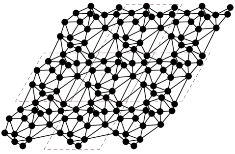
Figure 2: 2D approximation of the inhibitor. The diffusion potential is approximated by appropriate constants in disks and the diffusion flux between the disks by linear functions along the edges of the Delaunay triangulation.

A similar approximation can be extended to multidimensional reaction-diffusion equations [8]. In the present paper, we deal with 2D double periodic structures. Let $\mathbf{e}_{1}=(e_{1},0)$ and $\mathbf{e}_{2}=(e_{21},e_{22})$ be the translation vectors of the lattice $\mathcal{Q}=\{l_{1}\mathbf{e}_{1}+l_{2}\mathbf{e}_{2}:\;l_{j}\in\mathbb{Z}\}$ where $\mathbb{Z}$ denotes the set of integer numbers. Consider the periodic representative cell

$$Q_{0}=\{\mathbf{x}=t_{1}\mathbf{e}_{1}+t_{2}\mathbf{e}_{2}\},\;0<t_{j}<1\}.$$

For simplicity, we approximate the places of maximal diffusion potential by equal disks $D_{i}$ ($i=1,2,\ldots,N$) of radius $r$ centered at the set of points $\mathbf{A}=(\mathbf{a}_{1},\mathbf{a}_{2},\ldots,\mathbf{a}_{N})$ displayed in Fig.2. The maxima of the diffusion potential are approximated by disks and the minima by segments. Every line segment $P_{kj}$ is perpendicular to the segment $(\mathbf{a}_{k},\mathbf{a}_{j})$, its length holds $|P_{kj}|=2r$ and it is divided onto equal parts by $(\mathbf{a}_{k},\mathbf{a}_{j})$.

It is convenient to introduce new distance (metric) as follows. Two points $\mathbf{a},\mathbf{b}\in\mathbb{R}^{2}$ are identified if their difference $\mathbf{a}-\mathbf{b}=l_{1}\mathbf{e}_{1}+l_{2}\mathbf{e}_{2}$ belongs to the lattice $\mathcal{Q}$. Hence, the classic flat torus topology with the opposite sides welded is introduced on the cell $Q_{0}$. The distance $\|\mathbf{a}-\mathbf{b}\|$ between two points $\mathbf{a},\mathbf{b}\in Q_{0}$ is introduced as

$$\|\mathbf{a}-\mathbf{b}\|:=\min_{l_{1},l_{2}\in\mathbb{Z}}\left|\mathbf{a}-\mathbf{b}+l_{1}\mathbf{e}_{1}+l_{2}\mathbf{e}_{2}\right|,$$ (2.1)

where the modulus means the Euclidean distance in $\mathbb{R}^{2}$ between the points $\mathbf{a}$ and $\mathbf{b}$.

Construct the double periodic Voronoi diagram and the Delaunay triangulation corresponding to the set $\mathbf{A}$ on the torus $\mathcal{Q}_{0}=\cup_{l_{1},l_{2}\in\mathbb{Z}}(Q_{0}+l_{1}\mathbf{e}_{1}+l_{2}\mathbf{e}_{2})$. The edges of the Delaunay triangulation $E$ correspond to linear approximations of the diffusion flux between disks. The Delauney triangulation of the vertices $\mathbf{A}$ consists of straight lines connecting by pairs points of $\mathbf{A}$ belonging to neighbor Voronoi regions. Let the neighborhood relation between two vertexes be denoted by $\mathbf{a}_{j}\sim\mathbf{a}_{k}$ or shortly $j\sim k$. We call the constructed double periodic graph $(\mathbf{A},E)$ by the Delaunay graph.

Two graphs are called isomorphic if they contain the same number of vertices connected in the same way. One of the most important notation of the persent paper is the class of graphs $\mathcal{G}=\mathcal{G}_{(\mathbf{A},E)}$ isomorphic to the given graph $(\mathbf{A},E)$.

Let $\mathbf{u}=(u_{1},u_{2},\ldots,u_{N})$ denote the vector whose components are the maximal diffusion potentials in the corresponding disks. The discrete network model for densely packed disks [2], [6], [9] is based on the fact that the diffusion flux is concentrated in the necks between closely spaced inclusions having different potentials. In our model, closely spaced inclusions means the chain disk–segment–disk ($D_{k}\leftrightsquigarrow P_{kj}\leftrightsquigarrow D_{j}$) displayed in Fig.1b. For two neighbor disks $D_{k}$, $D_{j}$ with centers $\mathbf{a}_{k}$, $\mathbf{a}_{j}$ and a segment $P_{kj}$ between them the relative interparticle flux $g(|\mathbf{a}_{k}-\mathbf{a}_{j}|)$ can be approximated by Keller’s formula [5]

$$g(|\mathbf{a}_{k}-\mathbf{a}_{j}|)=\pi\sqrt{\frac{r}{\delta_{kj}}},$$ (2.2)

where $\delta_{kj}=\|\mathbf{a}_{k}-\mathbf{a}_{j}\|-2r$ denotes the gap between the neighbor disks. Keller’s formula (2.2) was deduced for the linear local diffusion flux between the neighbor disks that is agree with our approximation. Introduce the designation

$$\mathop{{\sum_{k,j}}^{(\mathcal{G})}}=\sum_{k=1}^{N}\sum_{j\sim k},$$ (2.3)

where $j\sim k$ means that the vertices $\mathbf{a}_{j}$ and $\mathbf{a}_{k}$ are connected. Following [2], [6] introduce the functional associated to the discrete energy

$$E(\mathbf{u},\mathbf{a})=\mathop{{\sum_{k,j}}^{(\mathcal{G})}}g(\|\mathbf{a}_{k}-\mathbf{a}_{j}\|)(u_{k}+u_{j})^{2},$$ (2.4)

where $u_{k}+u_{j}$ is the variation of the diffusion potential along the chain $D_{k}\leftrightsquigarrow P_{kj}\leftrightsquigarrow D_{j}$.

3 Optimal random packing

Consider the minimization problem

$$\mathcal{E}(\mathbf{u})=\min_{\mathbf{A}}\;E(\mathbf{u},\mathbf{A})=\min_{\mathbf{A}}\mathop{{\sum_{k,j}}^{(\mathcal{G})}}g(\|\mathbf{a}_{k}-\mathbf{a}_{j}\|)(u_{k}+u_{j})^{2}.$$ (3.1)

The function $g(x)=\pi\sqrt{\frac{r}{x-2r}}$ as a convex function satisfies Jensen’s inequality

$$\sum_{i=1}^{M}p_{i}g(x_{i})\geq g\left(\sum_{i=1}^{M}p_{i}x_{i}\right),$$ (3.2)

where the sum of positive numbers $p_{i}$ is equal to unity. Equality holds if and only if all $x_{i}$ are equal. Let the sum from (2.4) is arranged in such a way that $x_{i}=\|\mathbf{a}_{k}-\mathbf{a}_{j}\|$ and $p_{i}=\frac{1}{U}(u_{k}+u_{j})^{2}$, where $U=\mathop{{\sum}^{(\mathcal{G})}}(u_{k}+u_{j})^{2}$. Application of (3.2) to (2.4) yields

$$\mathop{{\sum}^{(\mathcal{G})}}g(\|\mathbf{a}_{k}-\mathbf{a}_{j}\|)(u_{k}+u_{j})^{2}\geq Ug\left(\frac{1}{U}\mathop{{\sum}^{(\mathcal{G})}}(u_{k}+u_{j})^{2}\|\mathbf{a}_{k}-\mathbf{a}_{j}\|\right).$$ (3.3)

Hölder’s inequality states that for non-negative $a_{i}$ and $b_{i}$

$$\sum_{i=1}^{M}a_{i}b_{i}\leq\left(\sum_{i=1}^{M}a_{i}^{2}\right)^{\frac{1}{2}}\left(\sum_{i=1}^{M}b_{i}^{2}\right)^{\frac{1}{2}}.$$ (3.4)

This implies that

$$\mathop{{\sum}^{(\mathcal{G})}}(u_{k}+u_{j})^{2}\|\mathbf{a}_{k}-\mathbf{a}_{j}\|\leq\left[\mathop{{\sum}^{(\mathcal{G})}}(u_{k}+u_{j})^{4}\right]^{\frac{1}{2}}\left[\mathop{{\sum}^{(\mathcal{G})}}\|\mathbf{a}_{k}-\mathbf{a}_{j}\|^{2}\right]^{\frac{1}{2}}.$$ (3.5)

The function $g(x)$ decreases, hence (3.3) and (3.5) give

$$\frac{1}{U}\mathop{{\sum}^{(\mathcal{G})}}g(\|\mathbf{a}_{k}-\mathbf{a}_{j}\|)(u_{k}+u_{j})^{2}\geq g\left(\frac{1}{U}\left[\mathop{{\sum}^{(\mathcal{G})}}(u_{k}+u_{j})^{4}\right]^{\frac{1}{2}}\left[\mathop{{\sum}^{(\mathcal{G})}}\|\mathbf{a}_{k}-\mathbf{a}_{j}\|^{2}\right]^{\frac{1}{2}}\right).$$ (3.6)

The minimum of the right hand part of (3.6) on $\mathbf{A}$ is achieved independently on $u_{k}$ for $\max_{\mathbf{A}}h(\mathbf{A})$ where

$$h(\mathbf{A})=\mathop{{\sum}^{(\mathcal{G})}}\|\mathbf{a}_{k}-\mathbf{a}_{j}\|^{2}.$$ (3.7)

Lemma 3.1 ([8]).

For any fixed class $\mathcal{G}_{(\mathbf{A}},E)$, every local maximizer of $h(\mathbf{A})$ is the global maximizer which fulfils the system of linear algebraic equations

$$\mathbf{a}_{k}=\frac{1}{N_{k}}\sum_{j\sim k}\mathbf{a}_{j}+\frac{1}{N_{k}}\sum_{\ell=1,2}s_{k\ell}\mathbf{e}_{\ell},\quad k=1,2,\ldots,N,$$ (3.8)

where $s_{k\ell}$ can take the values $0,\pm 1,\pm 2$ in accordance with the class $\mathcal{G}_{(\mathbf{A},E)}$. The system (3.8) has always a unique solution up to an additive arbitrary constant vector.

Equations (3.8) describe the stationary points of the functional (3.7) obtained by its differentiation on $\mathbf{a}_{k}$ ($k=1,2,\ldots,N$)

$$\sum_{j\sim k}(\mathbf{a}_{j}-\mathbf{a}_{k})\equiv\mathbf{0}.$$ (3.9)

Here, the congruence relation $\mathbf{a}\equiv\mathbf{b}$ means that $\mathbf{a}-\mathbf{b}=l_{1}\mathbf{e}_{1}+l_{2}\mathbf{e}_{2}$ for some integer $l_{1,2}$. Therefore, a point $\mathbf{a}$ on the torus $\mathcal{Q}_{0}$ is associated to the infinite set of points $\{\mathbf{a}+l_{1}\mathbf{e}_{1}+l_{2}\mathbf{e}_{2},\;l_{1,2}\in\mathbb{Z}\}$ on the plane $\mathbb{R}^{2}$. We now rewrite equation (3.9) on the torus as an equation on the plane for a fixed point $\mathbf{a}_{k}\in Q_{0}$. Consider a points $\mathbf{a}^{\prime}_{j}\in\mathbb{R}^{2}$ neighboring to $\mathbf{a}_{k}$, i.e., $j\sim k$ in a graph $(\mathbf{A},E)\in\mathcal{G}_{(\mathbf{A},E)}$. The point $\mathbf{a}^{\prime}_{j}$ is congruent to a point $\mathbf{a}_{j}\in Q_{0}$. The graph $(\mathbf{A},E)$ corresponds to the Voronoi tessellation, hence, $\mathbf{a}^{\prime}_{j}$ belongs to $Q_{0}$ or to neighbor cells $Q_{0}\pm\mathbf{e}_{1}$, $Q_{0}\pm\mathbf{e}_{2}$, $Q_{0}\pm\mathbf{e}_{1}\pm\mathbf{e}_{2}$. Therefore, $\mathbf{a}^{\prime}_{j}=\mathbf{a}_{j}+l_{1jk}\mathbf{e}_{1}+l_{2jk}\mathbf{e}_{2}$, where $l_{1jk}$ and $l_{2jk}$ can be equal only to $0,\pm 1$. Then, equations (3.9) can be written in the form (3.8) where

$$s_{1k}=\sum_{j\sim k}l_{1jk},\quad s_{2k}=\sum_{j\sim k}l_{2jk}.$$ (3.10)

One can see that the sum of all equations (3.8) gives an identity, hence, they are linearly dependent. Moreover, if $\mathbf{A}=(\mathbf{a}_{1},\mathbf{a}_{2},\ldots,\mathbf{a}_{N})$ is a solution of (3.8), then $(\mathbf{a}_{1}+\mathbf{c},\mathbf{a}_{2}+\mathbf{c},\ldots,\mathbf{a}_{N}+\mathbf{c})$ is also a solution of (3.8) for any $\mathbf{c}\in\mathbb{R}^{2}$. Let the point $\mathbf{a}_{N}$ be arbitrarily fixed. Then, $\mathbf{a}_{1},\mathbf{a}_{2},\ldots,\mathbf{a}_{N-1}$ can be found from the uniquely solvable system of linear algebraic equations

$$\mathbf{a}_{k}=\frac{1}{N_{k}}\sum_{j\sim k}\mathbf{a}_{j}+\frac{1}{N_{k}}\sum_{\ell=1,2}s_{k\ell}\mathbf{e}_{\ell},\quad k=1,2,\ldots,N-1.$$ (3.11)

It is worth noting that the system (3.11) can be decomposed onto two independent systems of scalar equations on the first and second coordinates of the points $\mathbf{a}_{1},\mathbf{a}_{2},\ldots,\mathbf{a}_{N-1}$.

4 Conclusion and numerical examples

We now proceed to summarize the algorithm to solve the optimization problem. First, let a class of graphs $\mathcal{G}_{(\mathbf{A},E)}$ be fixed with the corresponding translation vectors $\mathbf{e}_{1}$ and $\mathbf{e}_{2}$. Further, the constants $s_{k\ell}$ are constructed by the scheme described at the end of the previous section. The main numerical step is solution to the uniquely solvable system of linear algebraic equations (3.11) to construct vertices $\mathbf{A}$ and the corresponding double periodic Delaunay graph $(\mathbf{A},E)$. This graph is called optimal in the class $\mathcal{G}_{(\mathbf{A},E)}$. The optimal graph not necessary does correspond to a Voronoi tessellation. In this case, one can change a class of graphs by introduction of the new Voronoi tessellation for the vertices $\mathbf{A}$. Then, the set $\mathbf{A}$ will not necessary be optimal in the new class $\mathcal{G}^{\prime}_{\mathbf{A}}$. Let $(\mathbf{A}^{\prime},E^{\prime})$ be the optimal graph in the class $\mathcal{G}^{\prime}_{\mathbf{A}}$. Next, if the graph $(\mathbf{A}^{\prime},E^{\prime})$ does not correspond to a Voronoi tessellation, it can be ”improved” by $(\mathbf{A}^{\prime\prime},E^{\prime\prime})$ etc. Therefore, we arrive at the graph chain

$$(\mathbf{A},E)\to(\mathbf{A}^{\prime},E^{\prime})\to(\mathbf{A}^{\prime\prime},E^{\prime\prime})\to\cdots.$$ (4.1)

Example 4.1.

Consider the hexagonal lattice defined by the fundamental translation vectors $\mathbf{e}_{1}=\sqrt[4]{\frac{4}{3}}(1,0)$ and $\mathbf{e}_{2}=\sqrt[4]{\frac{4}{3}}(\frac{1}{2},\frac{\sqrt{3}}{2})$. The area of the cell $Q_{0}$ holds unit. Consider $N=3$ points $(1.075,0.175),(0.919,0.553),(0.444,0.169)$ and the corresponding double periodic Voronoi tessellation shown in Fig.3a.

Figure 3: a) Three points in the cell $Q_{0}$ are distinguished. Dashed lines show the lattice, solid lines the double periodic Delaunay graph. b) The optimal graph isomorphic to the graph from a).

Application of the algorithm yields the optimal hexagonal structure Fig.3b.

Example 4.2.

Consider the hexagonal lattice as in Example 4.1 and $N=16$ points with the corresponding double periodic Voronoi tessellation shown in Fig.2. The considered structure determines a double periodic graph $(\mathbf{A},E)$. This graph generates the class of isomorphic graphs $\mathcal{G}_{(\mathbf{A},E)}$. Find the optimal graph $(\mathbf{A}^{\prime},E)$ in the class $\mathcal{G}_{(\mathbf{A},E)}$. Construct the Voronoi tessellation corresponding to the set $\mathbf{A}^{\prime}$ and the corresponding graph $(\mathbf{A}^{\prime},E^{\prime})$ which determines the new class $\mathcal{G}^{\prime}_{(\mathbf{A}^{\prime},E^{\prime})}$. The optimal graph in the class $\mathcal{G}^{\prime}_{(\mathbf{A}^{\prime},E^{\prime})}$ is the graph $(\mathbf{A}^{\prime},E^{\prime})$. Therefore, in this example the graph $(\mathbf{A},E)$ from Fig.2 is transformed into the graph $(\mathbf{A}^{\prime},E^{\prime})$ from Fig.4.

Figure 4: The optimal graph $(\mathbf{A}^{\prime},E^{\prime})$ from Example 4.2.

Every edge of the Delaunay graph models the interaction caused by the diffusion flux. This flux between two disks can be insignificant if the gap between the disk is sufficiently large. In this case, the corresponding edge should be deleted from the Delaunay graph. We consider such a case in the following example.

Example 4.3.

Consider $N=9$ points and the double periodic Voronoi tessellation isomorphic to the hexagonal lattice. The perfect hexagonal array in Fig.5a presents the optimal graph $(\mathbf{A},E)$. Consider another graph $(\mathbf{A},E^{\prime})$ obtained from $(\mathbf{A},E)$ by deletion of the edges connecting the first layer of disks with other layers. In this case, the optimal graph becomes similar to hexagonal-layered structure displayed in Fig.5b.

Figure 5: The optimal graphs from Example 4.3. The disks in the layers 1 and 1’, 2 and 2’, 3 and 3’ are the same in the toroidal topology.

The above examples illustrate few scenarios of the 2D pattern formations. Systematic simulations can help to study properties of the optimal graphs. The main feature of the proposed method is investigation of the graph structures by analytical and numerical methods without treatment of PDE. The method of structural approximation recalls a finite element method when a continuous problem is approximated by a discrete problem. The structural approximation is based on a ”physical discretization” [2], when edges of the graph correspond to the most intensive places of the diffusion flux. Further, the principle of minimum energy yields a discrete numerical problem as in a finite element method. The method of structural approximation was justified for the $p-$Laplacian including linear equations in [2], [6], [9].

Remark 4.4.

Solution to the optimal energy problem yields solution to the optimal packing problem for disks [7], [8]. The corresponding concentration $\nu(\mathcal{G})$ of disks attains the maximal value in the class $\mathcal{G}_{(\mathbf{A},E)}$. The set of optimal graphs includes graphs corresponding to packing constructed by various packing protocols. This scheme gives the set of the optimal concentrations depending on protocols, i.e., on the class of graphs. Therefore, in order to get the set of all optimal packings, it is sufficient to determine the targets of the optimal locations (4.1). In the above examples, the graph chain (4.1) terminates. We cannot give an example with an infinite graph chain.

References

- [1] Bressloff, P.C. (2014) Stochastic processes in cell biology. Springer International Publishing Switzerland, New York etc.
- [2] Berlyand, L., Kolpakov, A.G., Novikov, A. (2013) Introduction to the Network Approximation. Method for Materials Modeling. Cambridge University Press, Cambridge.
- [3] Ghoniem, N., Walgraef, D. (2008) Instabilities and Self-Organization in Materials. Vol. 1,2, Oxford University Press, Oxford.
- [4] Jost, J. (2014) Mathematical Methods in Biology and Neurobiology. Springer, London etc.
- [5] Keller, J.B. (1963) Conductivity of a Medium Containing a Dense Array of Perfectly Conducting Spheres or Cylinders or Nonconducting Cylinders, J. Appl. Phys., 34, 991-993.
- [6] Kolpakov, A.A., Kolpakov, A.G. (2010) Capacity and Transport in Contrast Composite Structures: Asymptotic Analysis and Applications. CRC Press, Boca Raton.
- [7] Mityushev V., Rylko N. (2012) Optimal distribution of the non-overlapping conducting disks, Multiscale Model. Simul., 10, 180-190.
- [8] Mityushev V. (2014) Optimal packing of spheres in and extremal effective conductivity, arXiv:1412.7527.
- [9] Rylko N. (2008) Structure of the scalar field around unidirectional circular cylinders, Proc. R. Soc., A464, 391-407.
- [10] Tóth, L. Fejes (1953) Lagerungen in der Ebene auf der Kugel und im Raum. Springer-Verlag, Berlin etc.