An exact solution of the time-dependent Schrödinger equation with a rectangular potential for real and imaginary time

Abstract

A propagator for the one dimensional time-dependent Schrödinger equation with an asymmetric rectangular potential is obtained using the multiple-scattering theory approach. It allows for the consideration of the reflection and transmission processes as the particle scattering at the potential jump (in contrast to the conventional wave-like picture) and for accounting for the nonclassical counterintuitive contribution of the backward-moving component of the wave packet attributed to the particle. This propagator completely resolves the corresponding time-dependent Schrödinger equation (defines the wave function $\psi(x,t)$) and allows for considering the quantum mechanical effects of a particle reflection from the potential downward step/well and a particle tunneling through the potential barrier as a function of time. These results are related to fundamental issues such as measuring time in quantum mechanics (tunneling time, time of arrival, dwell time). For imaginary time, which represents an inverse temperature ($t\rightarrow-i\hbar/k_{B}T$), the obtained propagator is equivalent to the density matrix for a particle that is in a heat bath and is subject to a rectangular potential. This density matrix provides information on the particles’ density in the different spatial areas relative to the potential location and on the quantum coherences of the different particle spatial states. If one shifts to imaginary time ($t\rightarrow-it$), the matrix element of the calculated propagator in the spatial basis provides a solution to the diffusion-like equation with a rectangular potential. The obtained exact results are presented as the integrals from elementary functions and thus allow for a numerical visualization of the probability density $\left|\psi(x,t)\right|^{2}$, the density matrix and the solution of the diffusion-like equation. The results obtained may also be useful for spintronics applications due to the fact that the asymmetric (spin-dependent) rectangular potential can model the potential profile in layered magnetic nanostructures..

PACS numbers: 03.65.Nk, 03.65.Ta, 03.65.Xp

1 Introduction

We start with the one-dimensional Schrödinger equation for a particle of mass $m$ subject to potential $V(x)$

$$i\hbar\frac{\partial\psi(x;t)}{\partial t}=H\psi(x;t),$$ (1)

where $H$ is a self-adjoint operator

$$H=-\frac{\hbar^{2}}{2m}\frac{\partial^{2}}{\partial x^{2}}+V(x).$$ (2)

A solution to this equation can generally be presented as

$$\psi(x;t)=\int<x|K(t)|x^{\prime}>\psi(x^{\prime};0)dx^{\prime},$$ (3)

where $K(t)=\exp(-iHt/\hbar)$ is the propagator (Green’s function) for equation (1) in operator form and $<x|K(t)|x^{\prime}>$ is its matrix element in $x$-representation. Thus, the knowledge of the propagator provides the complete solution to the equation (1) at the given initial value $\psi(x^{\prime};0)$. If the initial value is of the form $\psi(x^{\prime};0)=\delta(x^{\prime}-x^{\prime\prime})$, the solution (3) reduces to the Green function matrix element

$$\psi(x,x^{\prime\prime};t)=<x|K(t)|x^{\prime\prime}>.$$ (4)

Equation (1) with an imaginary time variable is also relevant to other physical situations. If we make the substitutions $t\rightarrow-i\hbar\beta$ ($\beta=1/k_{B}T$) and $\psi(x,x^{\prime};-i\hbar\beta)\rightarrow\rho(x,x^{\prime};\beta)$, Eq. (4) represents the matrix element $\rho(x,x^{\prime};\beta)=<x|\exp(-\beta H)|x^{\prime}>$ of the density operator $\rho(\beta)=\exp(-\beta H)$, which satisfies the Bloch equation (in the $x$-representation)

$$\frac{\partial\rho(x,x^{\prime};\beta)}{\partial\beta}=-H\rho(x,x^{\prime};\beta),$$ (5)

with initial condition $\rho(x,x^{\prime};\beta=0)=\delta(x-x^{\prime})$ and where the operator $H$ (2) in (5) is applied only to the $x$ variable of the density matrix.

If we make the substitutions $t\rightarrow-it$, $\hbar\rightarrow 2mD$, $V(x)/2mD\rightarrow\overline{V}(x)$ and $\psi(x;-it)\rightarrow Q(x;t)$, Eq. (1) represents the inhomogeneous diffusion-like equation (with the diffusion coefficient $D$)

$$\frac{\partial Q(x;t)}{\partial t}=D\frac{\partial^{2}Q(x;t)}{\partial x^{2}}-\overline{V}(x)Q(x;t).$$ (6)

The solution to Eq. (6) at the initial condition $Q(x;0)=\delta(x-x_{0})$ is given by (4)

$$Q(x,x_{0};t)=<x|\exp(-Ht/2mD)|x_{0}>,$$ (7)

where $H$ is defined by (2) with $\hbar\rightarrow 2mD$.

We see that, in any case, the problem is to find a propagator of the type $<x|\exp(-\alpha H)|x^{\prime}>$ with different $\alpha$ for the considered parabolic differential equations.

A rectangular potential is the simplest one allowing for the study of some striking quantum mechanical effects, such as particle reflection from a potential step/well and transmission through a potential barrier. These phenomena are less surprising when we think of a wave being, e.g., reflected from a downward potential step, though they are more surprising from the particle point of view. They easily follow from the standard textbook stationary analysis, which reduces to substituting a plane wave of energy $E$ for the wave packet and solving the stationary Schrödinger equation. However, in this case, there are no real transport phenomena, i.e. in the absence of the energy dispersion ($\Delta E=0$) the transmission time through or the time of arrival (TOA) to the potential jumps is indefinite ($\Delta t\backsim\hbar/\Delta E$). It is interesting to verify the mentioned non-classical phenomena by considering the time-dependent picture of these processes in a realistic situation, when a particle, originally localized outside the potential well/barrier, moves towards the potential and experiences scattering at the potential jumps. In order to do this, the corresponding time-dependent Schrödinger equation needs to be solved. This problem is much more involved even in the one-dimensional case in comparison to the conventional stationary case.

In particular, there is one striking and classically forbidden counterintuitive (and often overlooked) effect even in the process of the simplest 1D time-dependent scattering by the mentioned potentials. A wave packet representing an ensemble of particles, confined initially (at $t=t_{0}$), say, somewhere to the region $x<0$, consists of both positive and negative momentum components due to the fact that a particle cannot be completely localized at $x<0$ if the wave packet contains only $p>0$ components. One would then expect that only particles with positive momenta $p$ may arrive at positive positions $x>0$ at $t>t_{0}$. However, the wave packet’s negative momentum components (restricted to a half line in momentum space) are necessarily different from zero in the whole $x$ space ($-\infty\div\infty$), representing the particles’ presence at $x>0$ at initial moment of time $t_{0}$, and, therefore, may contribute, for example, to the distribution of the particles’ time of arrival (TOA) to $x>0$ [1, 2]. It is worth noting that the contribution of the backward-moving (negative momentum) components in the initial-value problem is in some sense equivalent to the contribution of the negative energy (evanescent) components in the source solution [1]. Thus, the correct treatment of some aspects of the kinetics of the wave packet (even in the 1D case and even for a ”free” motion) becomes a nontrivial problem and is closely related to the fundamental problem of measuring time in quantum mechanics, such as TOA, the dwell time, and tunneling time.

In addition, the time-dependent aspects of reflection from and transmission through the potential step/barrier/well have recently acquired relevance not only in view of renewed interest in the fundamental problems of measuring time in quantum mechanics (see [3]), but also due to important practical applications in the newly emerged fields of nanoscience and nanotechnology. Rectangular (asymmetric spin-dependent) potential barriers/wells may often satisfactorily approximate the one-dimensional potential profiles in layered magnetic nanostructures (with sharp interfaces). In such nanostructures, the giant magnetoresistance (GMR) [4] and tunneling magnetoresistance (TMR) [5] effects occur.

The calculation of the propagator $<x|\exp(-\alpha H)|x^{\prime}>$ is conveniently related to the path-integral method (see, e.g. [6] and [7]). The list of the exact solutions for this propagator is very short. For example, there is an exact solution for the spacetime propagator $<x|\exp(-iHt/\hbar)|x^{\prime}>$ of the Schrödinger equation in the one-dimensional square barrier case obtained in [8], but this solution is very complicated, implicit and not easy to analyze (see also [9, 10, 11]).

Recently, we have suggested a simple method for the calculation of the spacetime propagator [12, 13, 14], which exactly resolves the time-dependent Schrödinger equation with a rectangular potential in terms of integrals of elementary functions. This method is an alternative to the commonly used path-integral approach to the mentioned problems and based on the energy integration of the spectral density matrix (discontinuity of the energy-dependent Green function across the real energy axis). The energy-dependent Green function is then easily obtained for the step/barrier/well potentials with multiple-scattering theory (MST) using the effective energy-dependent potentials found in [12], which are responsible for reflection from and transmission through the potential step. These potentials, which are defined via the different particle velocities from both sides of the potential steps making up the step/barrier/well potentials, allow for the consideration of the reflection and transmission processes as particle scattering at the potential jumps in contrast to the conventional wave-like picture. An important advantage of our approach is that the negative energy (evanescent states) contribution to the propagator cancels out due to the natural decomposition of the propagator into forward- and backward-moving components. This is an essential result because accounting for both of these components (which should generally be done) often leads to a rather complicated consideration of the evanescent states with $E<0$ (see [15]).

In this paper, we provide an exact solution to Eq. (1) for real and imaginary times using our approach [12, 13, 14] to the calculation of the spacetime propagator for a general asymmetric rectangular potential. In Sec. 2, we outline our MST approach to the calculation of the propagator for the time-dependent Schrödinger equation and present its explicit form. In Sec. 3, we consider a system in a heat bath, as is the case, e.g., for electrons in nanostructures. The equilibrium system’s characteristics can then be calculated knowing its density matrix $\rho(x,x^{\prime};\beta)=<x|\exp(-\beta H)|x^{\prime}>$. We present in this section an exact solution for the density matrix of a particle in an asymmetric (spin-dependent) one-dimensional rectangular potential and discuss its properties with the help of numerical evaluation of the corresponding integrals of elementary functions. In accordance with the above discussion of Eq. (1), the obtained solution for the spacetime propagator may be also used for finding the solution to the diffusion-like equation (1) through the appropriate change of the equation parameters. This case is discussed in Sec. 4 and the summary of the results is given in Sec. 5.

2 Multiple scattering calculation of a spacetime propagator for the Schrödinger equation

We start by considering a particle (electron) of mass $m$ in the following general asymmetric one-dimensional rectangular potential of width $d$ placed in the interval $0<x<d$

$$V(x)=[\theta(x)-\theta(x-d)]U+\theta(x-d)\Delta,$$ (8)

where $\theta(x)$ is the Heaviside step function, and the potential parameters $U$ and $\Delta$ can acquire positive as well as negative values (for $\Delta=U$, $V(x)$ reduces to the step potential). As an application, we can model by the potential (8) a spin-dependent potential profile of a threelayer made of a nonmagnetic spacer (metallic or insulator) sandwiched between two magnetic (infinite) layers, and the asymmetricity (spin-dependence) of the potential (8) is defined by the parameter $\Delta$. The particle wave vectors in different spatial areas (layers) are defined as

$$k_{<}^{0}(E) =k(E),k(E)=\sqrt{\frac{2m}{\hbar^{2}}E},x<0,$$

$$k_{>}^{0}(E) =k_{<}^{d}(E)=k_{u}(E),k_{u}(E)=\sqrt{\frac{2m}{\hbar^{2}}(E-U)},0<x<d,$$

$$k_{>}^{d}(E) =k_{\Delta}(E),k_{\Delta}(E)=\sqrt{\frac{2m}{\hbar^{2}}(E-\Delta)},x>d.$$ (9)

In the case of three-dimensional sandwiches, $k_{>(<)}^{0}(E)$ and $k_{>(<)}^{d}(E)$ are the perpendicular-to-interface components of the wave vector $\mathbf{k}$ of a particle arriving at the interfaces (located at $x=0$ and $x=d$) from the right ($>$) or from the left ($<$).

The wave function of a single particle moving in perturbing potential $V(x)$ is given by Eq. (3) (see also [6]). The propagator $K(x,x^{\prime};t)=<x|\exp(-iHt/\hbar)|x^{\prime}>$ is the probability amplitude for particle transition from the initial spacetime point ($x^{\prime},0$) to the final point ($x,t$) by means of all possible paths. It provides full information on the particle’s dynamics and resolves the corresponding time-dependent Schrödinger equation (1). According to [12], the time-dependent retarded propagator $K(t)=\theta(t-t^{\prime})\exp(-\frac{i}{\hbar}Ht)$ can be represented as

$$K(t)=\theta(t)\frac{i}{2\pi}{\displaystyle\int\limits_{-\infty}^{\infty}}dEe^{-\frac{i}{\hbar}Et}(\frac{1}{E-H+i\varepsilon}-\frac{1}{E-H-i\varepsilon}),\varepsilon\rightarrow+0,$$ (10)

where $H$ is the time-independent Hamiltonian of the system under consideration. Equation (10) follows either from the contour integration in the complex plane or from the identity

$$\frac{1}{E-H\pm i\varepsilon}=P\frac{1}{E-H}\mp i\pi\delta(E-H),$$ (11)

where $P$ is the symbol of the integral principal value. In the space representation (10) reads

$$K(x,x^{\prime};t)=\theta(t){\displaystyle\int\limits_{-\infty}^{\infty}}e^{-\frac{i}{\hbar}Et}A(x,x^{\prime};E)dE.$$ (12)

Here $A(x,x^{\prime};E)$ is the spectral density matrix

$$A(x,x^{\prime};E) =\frac{i}{2\pi}\left[G^{+}(x,x^{\prime};E)-G^{-}(x,x^{\prime};E)\right],$$

$$G^{+}(x,x^{\prime};E) =<x|\frac{1}{E-H+i\varepsilon}|x^{\prime}>,G^{-}(x,x^{\prime};E)=\left[G^{+}(x^{\prime},x;E)\right]^{\ast},\varepsilon\rightarrow+0,$$ (13)

determined by the matrix elements of the retarded $G^{+}(E)$ and advanced $G^{-}(E)$ energy-dependent operator Green functions $G^{\pm}=(E-H\pm i\varepsilon)^{-1}$, which are analytical in the upper and lower half-planes of the complex energy $E$, respectively. The propagator in the form of (12) is a useful tool for calculations within the multiple-scattering theory (MST) perturbation expansion if the Hamiltonian can be split as $H=H_{0}+H_{i}$, where $H_{0}$ describes a free motion and $H_{i}$ is the scattering potential. Note, that in this case one would not need rely on the standard (often cumbersome) matching procedure characteristic of the picture when a wave (representing a particle) is reflected from and transmitted through the potential (8). On the other hand, the introduction of the scattering potential $H_{i}$ corresponds to the natural picture of the particle scattering at the potential jumps at $x=0$ and $x=d$.

We showed in [12] that the Hamiltonian corresponding to the energy-conserving processes of scattering at potential steps can be presented as

$$H =H_{0}+H_{i}(x;E),$$

$$H_{i}(x;E) ={\displaystyle\sum\limits_{s}}H_{i}^{s}(E)\delta(x-x_{s}).$$ (14)

Here, $H_{i}(x;E)$ describes the perturbation of the ”free” particle motion (defined by $H_{0}=-\frac{\hbar^{2}}{2m}\frac{\partial^{2}}{\partial x^{2}}$) localized at the potential steps with coordinates $x_{s}$ (in the case of the potential (8), there are two potential steps at $x_{s}=0$ and $x_{s}=d$)

$$H_{i>}^{s}(E) =\frac{i\hbar}{2}[v_{>}^{s}(E)-v_{<}^{s}(E)],$$

$$H_{i<}(E) =\frac{i\hbar}{2}[v_{<}^{s}(E)-v_{>}^{s}(E)],$$

$$H_{i><}(E) =\frac{2i\hbar v_{>}^{s}(E)v_{<}^{s}(E)}{[\sqrt{v_{>}^{s}(E)}+\sqrt{v_{<}^{s}(E)}]^{2}},$$ (15)

where $H_{i>(<)}^{s}(E)$ is the reflection (from the potential step at $x=x_{s}$) potential amplitude, the index $>(<)$ indicates the side on which the particle approaches the interface at $x=x_{s}$: right ($>$) or left ($<$); $H_{i><}^{s}(E)$ is the transmission potential amplitude, and the velocities $v_{>(<)}^{s}(E)=\hbar k_{>(<)}^{s}(E)/m,s\in\{0,d\}$ ($k_{>(<)}^{s}(E)$ are given by (9)).

The perturbation expansion for the retarded Green function $G^{+}(x,x^{\prime};E)$ in the case of the rectangular potential (8), which can be effectively represented by the two-step effective scattering Hamiltonian (14), reads for different source (given by $x^{\prime}$) and destination (determined by $x$) areas of interest as

$$G^{+}(x,x^{\prime};E) =G_{0}^{+}(x,d;E)T^{+}(E)G_{0}^{+}(0,x^{\prime};E),x^{\prime}<0,x>d,$$

$$G^{+}(x,x^{\prime};E) =G_{0}^{+}(x,0;E)T^{+}(E)G_{0}^{+}(d,x^{\prime};E),x^{\prime}>d,x<0,$$

$$G^{+}(x,x^{\prime};E) =G_{0}^{+}(x,0;E)T^{\prime+}(E)G_{0}^{+}(0,x^{\prime};E)+G_{0}^{+}(x,d;E)R^{\prime+}(E)G_{0}^{+}(0,x^{\prime};E),x^{/}<0,0<x<d,$$

$$G^{+}(x,x^{\prime};E) =G_{0}^{+}(x,0;E)T^{\prime+}(E)G_{0}^{+}(0,x^{\prime};E)+G_{0}^{+}(x,0;E)R^{\prime+}(E)G_{0}^{+}(d,x^{\prime};E),0<x^{/}<d,x<0,$$

$$G^{+}(x,x^{\prime};E) =G_{0}^{+}(x,x^{\prime};E)+G_{0}^{+}(x,0;E)R^{+}(E)G_{0}^{+}(0,x^{\prime};E),x^{\prime}<0,x<0,$$ (16)

where the transmission and reflection matrices are

$$T^{+}(E) =\frac{T_{><}^{d+}(E)G_{0}^{+}(d,0;E)T_{><}^{0+}(E)}{D^{+}(E)},$$

$$T^{\prime+}(E) =\frac{T_{><}^{0+}(E)}{D^{+}(E)},R^{\prime+}(E)=T_{<}^{d+}(E)G_{0}^{+}(d,0;E)T^{\prime+}(E),$$

$$R^{+}(E) =T_{<}^{0+}(E)+\frac{T_{><}^{0+}(E)G_{0}^{+}(0,d;E)T_{<}^{d+}(E)G_{0}^{+}(d,0;E)T_{><}^{0+}(E)}{D^{+}(E)},$$

$$D^{+}(E) =1-T_{<}^{d+}(E)G_{0}^{+}(d,0;E)T_{>}^{0+}(E)G_{0}^{+}(0,d;E).$$ (17)

The one-dimensional retarded Green function $G_{0}^{+}(x,x^{\prime};E)$ corresponding to a free particle moving in constant potential $V(x)=0$ or $V(x)=U($or $\Delta)$ is (see, e.g. [17])

$$G_{0}^{+}(x,x^{\prime};E) =\frac{m}{i\hbar^{2}k(E)}\exp[ik(E)|x-x^{\prime}|],V(x)=0,$$

$$G_{0}^{+}(x,x^{\prime};E) =\frac{m}{i\hbar^{2}k_{u(\Delta)}(E)}\exp[ik_{u(\Delta)}(E)|x-x^{\prime}|],V(x)=U(\text{or }\Delta),$$ (18)

where the wave numbers are determined by (9). The scattering (at the step located at $x=x_{s}$) t-matrices are defined by the following perturbation expansion

$$T^{s}(E) =H_{i}^{s}(E)+H_{i}^{s}(E)G_{0}(x_{s},x_{s};E)H_{i}^{s}(E)+\ldots$$

$$=\frac{H_{i}^{s}(E)}{1-G_{0}(x_{s},x_{s};E)H_{i}^{s}(E)},$$ (19)

where $H_{i}^{s}(E)$ and the interface Green function $G_{0}(x_{s},x_{s};E)$ are defined differently for reflection and transmission processes [12]: the step-localized effective potential is given by Eq. (15) and the retarded Green functions at the interface for the considered reflection and transmission processes are, correspondingly,

$$G_{0>(<)}^{+}(x_{s},x_{s};E) =1/i\hbar v_{>(<)}^{s}(E)$$

$$G_{0><}^{+}(x_{s},x_{s};E) =1/i\hbar\sqrt{v_{>}^{s}(E)v_{<}^{s}(E)}$$ (20)

in accordance with (18).

From (15), (19) and (20), we have for the reflection $T_{>(<)}^{s+}(E)$ and transmission $T_{><}^{s+}(E)$ t-matrices, used in (17) ($s\in\{0,d\}$) and corresponding to the retarded Green function and scattering at the interface located at $x=x_{s}\in\{0,d\}$:

$$T_{>(<)}^{s+}(E) =i\hbar v_{>(<)}^{s}r_{>(<)}^{s},$$

$$T_{><}^{s+}(E) =i\hbar\sqrt{v_{>}^{s}v_{<}^{s}}t^{s},$$ (21)

where $r_{>(<)}^{s}(E)$ and $t^{s}(E)$ are the standard amplitudes for reflection to the right (left) of the potential step at $x=x_{s}$ and transmission through this step

$$r_{>}^{s}(E) =\frac{k_{>}^{s}-k_{<}^{s}}{k_{>}^{s}+k_{<}^{s}},r_{<}^{s}(E)=\frac{k_{<}^{s}-k_{>}^{s}}{k_{>}^{s}+k_{<}^{s}},$$

$$t^{s}(E) =\frac{2\sqrt{k_{>}^{s}k_{<}^{s}}}{k_{>}^{s}+k_{<}^{s}},$$ (22)

and the argument $E$ is omitted for brevity.

Now, using (9), (16), (17), (18), (21) and (22), we can obtain the Green function $G^{+}(x,x^{\prime};E)$ for the spatial domains considered in (16) (see [16])

$$G^{+}(x,x^{\prime};E) =\frac{m}{i\hbar^{2}\sqrt{kk_{\Delta}}}e^{ik_{\Delta}(x-d)}t(E)e^{-ikx^{\prime}},x^{\prime}<0,x>d,$$

$$G^{+}(x,x^{\prime};E) =\frac{m}{i\hbar^{2}\sqrt{kk_{\Delta}}}e^{-ikx}t(E)e^{ik_{\Delta}(x^{\prime}-d)},x^{\prime}>d,x<0,$$

$$G^{+}(x,x^{\prime};E) =\frac{m}{i\hbar^{2}\sqrt{kk_{u}}}\left[e^{ik_{u}x}t^{\prime}(E)e^{-ikx^{\prime}}+e^{-ik_{u}x}r^{\prime}(E)e^{-ikx^{\prime}}\right],x^{\prime}<0,0<x<d,$$

$$G^{+}(x,x^{\prime};E) =\frac{m}{i\hbar^{2}\sqrt{kk_{u}}}\left[e^{-ikx}t^{\prime}(E)e^{ik_{u}x^{\prime}}+e^{-ikx}r^{\prime}(E)e^{-ik_{u}x^{\prime}}\right],x<0,0<x^{\prime}<d,$$

$$G^{+}(x,x^{\prime};E) =\frac{m}{i\hbar^{2}k}\left[e^{ik\left|x-x^{\prime}\right|}+r(E)e^{-ik(x+x^{\prime})}\right],x<0,x^{\prime}<0,$$ (23)

where the transmission and reflection amplitudes are defined as

$$t(E) =\frac{4\sqrt{kk_{\Delta}}k_{u}e^{ik_{u}d}}{d(E)},t^{\prime}(E)=\frac{2\sqrt{kk_{u}}(k_{\Delta}+k_{u})}{d(E)},$$

$$r^{\prime}(E) =\frac{2\sqrt{kk_{u}}(k_{u}-k_{\Delta})e^{2ik_{u}d}}{d(E)},r(E)=\frac{(k-k_{u})(k_{\Delta}+k_{u})-(k+k_{u})(k_{\Delta}-k_{u})e^{2ik_{u}d}}{d(E)},$$

$$d(E) =(k+k_{u})(k_{\Delta}+k_{u})-(k-k_{u})(k_{\Delta}-k_{u})e^{2ik_{u}d}.$$ (24)

Using the same approach, it is not difficult to obtain the Green function $G^{+}(x,x^{\prime};E)$ for other areas of arguments $x$ and $x^{\prime}$.

In accordance with the obtained results for Green’s functions, we consider the situation when a particle, given originally by a wave packet localized to the left of the potential area, i.e. at $x^{\prime}<0$, moves towards the potential (8). We also choose $\Delta\geqslant 0$, which corresponds to the case when, e.g., the spin-up electrons of the left magnetic layer ($x^{\prime}<0$) move through the nonmagnetic spacer to the right magnetic layer ($x>d$) aligned either in parallel ($\Delta=0$) or antiparallel ($\Delta>0$) to the left magnetic layer. At the same time, the amplitude $U$ in the potential (8) may acquire both positive (barrier) and negative (well) values.

From Eqs. (23) we see that $G^{+}(x,x^{\prime};E)=G^{+}(x^{\prime},x;E)$, and, therefore, the advanced Green function $G^{-}(x,x^{\prime};E)=\left[G^{+}(x^{\prime},x;E)\right]^{\ast}=\left[G^{+}(x,x^{\prime};E)\right]^{\ast}$ (see, e.g. [17]). Thus, the transmission amplitude (12) is determined by the imaginary part of the Green function and can be written as

$$K(x,x^{\prime};t)=-\theta(t)\frac{1}{\pi}{\displaystyle\int\limits_{-\infty}^{\infty}}dEe^{-\frac{i}{\hbar}Et}\operatorname{Im}G^{+}(x,x^{\prime};E).$$ (25)

Formulas (23) - (25) present the exact solution for the particle propagator in the presence of the potential (8). It should be kept in mind that the wave numbers (9) and, therefore, the quantities $t(E)$, $t^{\prime}(E)$, $r^{\prime}(E)$, and $r(E)$ in (24) are different in the ${\displaystyle\int\limits_{-\infty}^{0}}dE$ and ${\displaystyle\int\limits_{0}^{\infty}}dE$ energy integration areas: in the former case, $k(E)$ and $k_{\Delta}(E)$ ($\Delta\geqslant 0$) should be replaced with $i\overline{k}(E)$ and $i\overline{k}_{\Delta}(E)$, where $\overline{k}(E)=\sqrt{-2mE/\hbar^{2}}$ ($E<0$) and $\overline{k}_{\Delta}(E;\mathbf{k}_{||})=\sqrt{2m(\Delta-E)/\hbar^{2}}$. At the same time, for energies $E<0$, the wave number $k_{u}=i\overline{k}_{u}$, $\overline{k}_{u}=\sqrt{2m(U-E)/h^{2}}$, for $U>0$ (barrier), but for $U<0$ it is real, i.e. $k_{u}=\sqrt{2m(E+\left|U\right|)/\hbar^{2}}$, if $E>-\left|U\right|$ and $k_{u}=i\overline{k}_{u}$, $\overline{k}_{u}=\sqrt{-2m(E+\left|U\right|)/\hbar^{2}}$ if $E<-\left|U\right|$. It follows that the ”free” Green function $G_{0}^{+}(x,x^{\prime};E)=\frac{m}{i\hbar^{2}k}e^{ik\left|x-x^{\prime}\right|}$ is real in the energy interval ($-\infty\div 0$) and, therefore, does not contribute in this interval to the corresponding ”free” propagator $K_{0}(x,x^{\prime};t)$ defined by (25). It is also remarkable that for energies $E<0$ the imaginary parts of the Green functions vanish in all spatial regions, as is seen from definitions (23) and (24) (e.g., $\operatorname{Im}t(E)=0$ and $\operatorname{Im}r(E)=0$ for $E<0$). Therefore, the energy interval ($-\infty\div 0$) does not contribute to the propagation of the particles through the potential well/barrier region. Thus, we have for $t>0$

$$K(x,x^{\prime};t) =\frac{1}{\pi\hbar}{\displaystyle\int\limits_{0}^{\infty}}\frac{dEe^{-\frac{i}{\hbar}Et}}{\sqrt{v(E)}}\operatorname{Re}\left[\frac{t(E)e^{ik_{\Delta}(E)(x-d)}e^{-ik(E)x^{\prime}}}{\sqrt{v_{\Delta}(E)}}\right],x^{\prime}<0,x>d,$$

$$K(x,x^{\prime};t) =\frac{1}{\pi\hbar}{\displaystyle\int\limits_{0}^{\infty}}\frac{dEe^{-\frac{i}{\hbar}Et}}{\sqrt{v(E)}}\operatorname{Re}\left\{\frac{e^{-ik(E)x^{\prime}}\left[t^{\prime}(E)e^{ik_{u}(E)x}+r^{\prime}(E)e^{-ik_{u}(E)x}\right]}{\sqrt{v_{u}(E)}}\right\},x^{\prime}<0,0<x<d,$$

$$K(x,x^{\prime};t) =\frac{1}{\pi\hbar}{\displaystyle\int\limits_{0}^{\infty}}\frac{dEe^{-\frac{i}{\hbar}Et}}{v(E)}\operatorname{Re}[e^{ik(E)\left|x-x^{\prime}\right|}+r(E)e^{-ik(E)(x+x^{\prime})}],x^{\prime}<0,x<0,$$ (26)

where the velocities $v(E)$, $v_{u}(E)$ and $v_{\Delta}(E)$ are defined by (9) with the multiplier $\hbar/m$.

It is easy to verify that the integration over $E$ of the first term in the last line of (26) results in the known formula for the space-time propagator for a freely moving particle

$$K_{0}(x,x^{\prime};t)=(\frac{m}{2\pi i\hbar t})^{1/2}\exp\left[\frac{im(x-x^{\prime})^{2}}{2\hbar t}\right],x<0,x^{\prime}<0.$$ (27)

The obtained results (26) for the particle propagator completely resolve (by means of Eq. (3)) the time-dependent Schrödinger equation for a particle moving under the influence of the rectangular potential (8). The form of this solution (integrals from the elementary functions) is convenient for numerical visualization. Further application of these results to the calculation of the TOA and dwell time as well as of the probability density of finding a particle in different spatial areas as a function of time with account of the forward- and backward-moving components of the wave function and their interference can be found in our earlier papers [12, 13, 14, 16].

3 Application to the density matrix

The equilibrium non-normalized density operator (propagator in the temperature domain) $\rho(\beta)=\exp(-\beta H)$ can likewise be expressed in terms of the resolvent operator $(E-H)^{-1}$ (see (10))

$$\rho(\beta)=\exp(-\beta H)=\frac{i}{2\pi}\int\limits_{-\infty}^{\infty}dEe^{-\beta E}(\frac{1}{E-H+i\varepsilon}-\frac{1}{E-H-i\varepsilon}).$$ (28)

Particularly, in the coordinate representation we have for the density matrix (see (4))

$$\rho(x,x^{\prime};\beta)=\int\limits_{-\infty}^{\infty}e^{-\beta E}A(x,x^{\prime};E)dE,$$ (29)

where $A(x,x^{\prime};E)$ is given by (13). Thus, the density matrix $\rho(x,x^{\prime};\beta)$ follows from the propagator (12) by the substitution $t\rightarrow-i\hbar\beta$ ($\beta=1/k_{B}T$). From the properties (13) we see that the density matrix (29) is self-adjoint. The density operator (28) satisfies the Bloch equation (5).

Thus, shifting to the imaginary ”time” ($t\rightarrow-i\hbar\beta$), we obtain the exact density matrix $\rho(x,x^{\prime};\beta)$ in the various considered (relative to the potential (8) area) spatial regions, i.e.

$$\rho(x,x^{\prime};\beta)=K(x,x^{\prime};-i\hbar\beta),$$ (30)

where $K(x,x^{\prime};t=-i\hbar\beta)$ is given by (26). In particular, we obtain from (27) the known result for the ”free” density matrix

$$\rho_{0}(x,x^{\prime};\beta)=K_{0}(x,x^{\prime};-i\hbar\beta)=(\frac{m}{2\pi\hbar^{2}\beta})^{1/2}\exp[-\frac{m(x-x^{\prime})^{2}}{2\hbar^{2}\beta}].$$ (31)

Using the same approach, it is not difficult to obtain the propagator $\rho(x,x^{\prime};\beta)$ for other (than in (26)) areas of the arguments $x$ and $x^{\prime}$. Again, it is important to note that the negative energy half line ($-\infty\div 0$), corresponding to the evanescent states does not contribute to the propagator (29). The diagonal element $K(x,x;\beta)$ ($x=x^{\prime}$ can be put only in the last line of (26)) defines the density of particles per unit length at the point $x<0$ to the left of the potential (8). The nondiagonal elements $K(x,x^{\prime};\beta)$ of (26) are related to the quantum mechanical interference effects. Particularly, they are responsible for particle tunneling through the barrier and also can be attributed to the phase correlation of the states $|x>$ and $|x^{\prime}>$.

Equations (26) and (30) provide an exact solution for the particle density matrix in the presence of the rectangular potential (8) in terms of integrals of elementary functions. It is convenient (e.g., for numerical visualization of the obtained results) to shift to dimensionless variables. As seen from (8), (9) and (26), there are the natural spatial scale $d$ and the energy scale $E_{d}=\hbar^{2}/2md^{2}$ (the energy uncertainty due to particle localization within a potential range of width $d$). Then, the density matrix (30) in the different spatial regions can be presented in the dimensionless variables as

$$\rho(\widetilde{x},\widetilde{x}^{\prime};\widetilde{\beta}) =\frac{1}{2\pi d}\int\limits_{0}^{\infty}\frac{d\widetilde{E}e^{-\widetilde{\beta}\widetilde{E}}}{\widetilde{E}^{1/4}}\operatorname{Re}\left[\frac{\widetilde{t}(\widetilde{E})e^{i\sqrt{\widetilde{E}-\widetilde{\Delta}}(\widetilde{x}-1)}e^{-i\sqrt{\widetilde{E}}\widetilde{x}^{\prime}}}{(\widetilde{E}-\widetilde{\Delta})^{1/4}}\right],\widetilde{x}^{\prime}<0,\widetilde{x}>1,$$

$$\rho(\widetilde{x},\widetilde{x}^{\prime};\widetilde{\beta}) =\frac{1}{2\pi d}\int\limits_{0}^{\infty}\frac{d\widetilde{E}e^{-\widetilde{\beta}\widetilde{E}}}{\widetilde{E}^{1/4}}\operatorname{Re}\left\{\frac{\left[\widetilde{t}^{\prime}(\widetilde{E})e^{i\sqrt{\widetilde{E}-\widetilde{U}}\widetilde{x}}+\widetilde{r}^{\prime}(\widetilde{E})e^{-i\sqrt{\widetilde{E}-\widetilde{U}}\widetilde{x}}\right]e^{-i\sqrt{\widetilde{E}}\widetilde{x}^{\prime}}}{(\widetilde{E}-\widetilde{U})^{1/4}}\right\},\widetilde{x}^{\prime}<0,0<\widetilde{x}<1,$$

$$\rho(\widetilde{x},\widetilde{x}^{\prime};\widetilde{\beta}) =\frac{1}{2\sqrt{\pi\widetilde{\beta}}d}\exp[-(\widetilde{x}-\widetilde{x}^{\prime})^{2}/4\widetilde{\beta}]+\frac{1}{2\pi d}\int\limits_{0}^{\infty}\frac{d\widetilde{E}e^{-\widetilde{\beta}\widetilde{E}}}{\sqrt{\widetilde{E}}}\operatorname{Re}[\widetilde{r}(\widetilde{E})e^{=i\sqrt{\widetilde{E}}(\widetilde{x}+\widetilde{x}^{\prime})}],\widetilde{x}^{\prime}<0,\widetilde{x}<0,$$ (32)

where

$$\widetilde{t}(\widetilde{E}) =\frac{4\widetilde{E}^{1/4}(\widetilde{E}-\widetilde{\Delta})^{1/4}\sqrt{\widetilde{E}-\widetilde{U}}e^{i\sqrt{\widetilde{E}-\widetilde{U}}}}{\widetilde{d}(\widetilde{E})},$$

$$\widetilde{t}^{\prime}(\widetilde{E}) =\frac{2\widetilde{E}^{1/4}(\widetilde{E}-\widetilde{U})^{1/4}(\sqrt{\widetilde{E}-\widetilde{\Delta}}+\sqrt{\widetilde{E}-\widetilde{U}})}{\widetilde{d}(\widetilde{E})},$$

$$\widetilde{r}^{\prime}(\widetilde{E}) =\frac{2\widetilde{E}^{1/4}(\widetilde{E}-\widetilde{U})^{1/4}(\sqrt{\widetilde{E}-\widetilde{U}}-\sqrt{\widetilde{E}-\widetilde{\Delta}})e^{2i\sqrt{\widetilde{E}-\widetilde{U}}}}{\widetilde{d}(\widetilde{E})},$$

$$\widetilde{r}(\widetilde{E}) =\frac{(\sqrt{\widetilde{E}}-\sqrt{\widetilde{E}-\widetilde{U}})(\sqrt{\widetilde{E}-\widetilde{\Delta}}+\sqrt{\widetilde{E}-\widetilde{U}})-(\sqrt{\widetilde{E}}+\sqrt{\widetilde{E}-\widetilde{U}})(\sqrt{\widetilde{E}-\widetilde{\Delta}}-\sqrt{\widetilde{E}-\widetilde{U}})e^{2i\sqrt{\widetilde{E}-\widetilde{U}}}}{\widetilde{d}(\widetilde{E})},$$

$$\widetilde{d}(\widetilde{E}) =(\sqrt{\widetilde{E}}+\sqrt{\widetilde{E}-\widetilde{U}})(\sqrt{\widetilde{E}-\widetilde{\Delta}}+\sqrt{\widetilde{E}-\widetilde{U}})-(\sqrt{\widetilde{E}}-\sqrt{\widetilde{E}-\widetilde{U}})(\sqrt{\widetilde{E}-\widetilde{\Delta}}-\sqrt{\widetilde{E}-\widetilde{U}})e^{2i\sqrt{\widetilde{E}-\widetilde{U}}},$$ (33)

and $\widetilde{E}=E/E_{d}$, $\widetilde{U}=U/E_{d}$, $\widetilde{\Delta}=\Delta/E_{d}$, $\widetilde{\beta}=E_{d}/k_{B}T=\widetilde{T}/T$, $\widetilde{T}=E_{d}/k_{B}$, $\widetilde{x}=x/d$, $\widetilde{x}^{\prime}=x^{\prime}/d$.

We will visualize the results given by Eqs. (32) and (33) for several specific values of the relevant parameters. For an electron and the potential width $d=10^{-7}cm$ ($1nm$), the characteristic energy $E_{d}\sim 3\cdot 10^{-2}ev$ and the characteristic temperature $\widetilde{T}=E_{d}/k_{B}\backsim 3\cdot 10^{2}K$.

We will perform the numerical modeling of the density matrix (32) with the symmetric rectangular potential (8) when $\Delta=0$ (in this case the transition and reflection amplitudes (33) simplify essentially). To secure a rapid convergence of the integrals in (32), we consider low enough temperatures, i.e. put $\widetilde{\beta}=10$ ($k_{B}T\ll E_{d}$). Figure 1 shows the diagonal element of the density matrix $\rho(\widetilde{x},\widetilde{x};\widetilde{\beta})$ (the last line in (32)) at $\widetilde{x}=-2$, i.e. the probability density to find a particle at this spatial point to the left of the barrier as a function of the potential well modulus $\left|\widetilde{U}\right|$ ($\widetilde{U}=0\div-300$). We see that in this case the density matrix $\rho(\widetilde{x},\widetilde{x};\widetilde{\beta})$ exhibits a series of maximums and minimums. This can be explained by the formation of the resonance levels above the well if the condition $\widetilde{E}+\left|\widetilde{U}\right|=\pi^{2}n^{2}$ ($n$ is integer, $n=1,2,\ldots$) holds. With such a condition we have the reflection amplitude $\widetilde{r}(\widetilde{E})=0$ and the transmission amplitude $\widetilde{t}(\widetilde{E})=\pm 1$. As at low temperatures ($\widetilde{\beta}=10$) the main contribution to the integral over $\widetilde{E}$ comes from the small (close to zero) energies, the positions of jumps at Fig. 1 approximately follow the relation $\left|\widetilde{U}\right|=\pi^{2}n^{2}$ ($n=1,2,\ldots$).

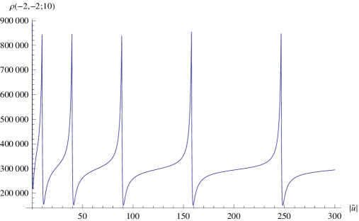
Figure 1: The diagonal element $\rho(-2,-2;10)$ as a function of the depth of the potential well $\left|\widetilde{U}\right|$.

The same diagonal element $\rho(-2,-2;10)$ as a function of the height of the potential barrier $\widetilde{U}=0\div 300$ behaves quite different from the case of the potential well and is shown in Fig. 2. One can see that the particle probability density at the given point to the left of the barrier $\widetilde{x}=-2$ exhibits at first a steep fall with the potential barrier growth and then it changes slowly with $\widetilde{U}$.

Figure 2: The same (as in Fig. 1) diagonal element of the density matrix as a function of the potential barrier height $\widetilde{U}$.

We will evaluate the nondiagonal elements of the density matrix $\rho(\widetilde{x},\widetilde{x}^{\prime};\widetilde{\beta})$ for points at different sides of the well/barrier (the first line in (32)) as a function of the potential parameter $\widetilde{U}$. Thus, we put $\widetilde{x}^{\prime}=-10$ (before the potential), $\widetilde{x}=2$ (beyond the potential) and $\widetilde{\beta}=10$ (as for Figs. (8) and (9)). Figure 3 exhibits the picks from the density matrix for the case of the potential well with $\widetilde{U}=0\div-300$ at the resonance values of $\left|\widetilde{U}\right|$ which correspond to the minima in Fig. 1.

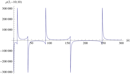
Figure 3: The nondiagonal element of the density matrix $\rho(2,-10;10)$ as a function of the potential well depth $\left|\widetilde{U}\right|$.

We see that in this case ($\widetilde{U}<0$) the density matrix nondiagonal elements can acquire both positive and negative values. Note that at $\widetilde{U}=0$ the density matrix reduces to the free density matrix (31) and therefore is positive (the seemingly negative value of the density matrix close to $\widetilde{U}=0$ in Fig. 3 is due to small resolution on the $\left|\widetilde{U}\right|$-axis; calculation on the smaller scale near the point $\widetilde{U}=0$ shows that at $\widetilde{U}=0$ the density matrix is positive). Thus, Fig. 3 demonstrates the jumps of the quantum coherence between the particle states before ($x^{\prime}<0$) and beyond ($x>0$) the potential well at the resonance particle transmission through the potential well. At the values of $\left|\widetilde{U}\right|$ that do not satisfy the resonance condition this quantum coherence is small.

The nondiagonal matrix element $\rho(2,-10;10)$ as a function of the potential barrier height ($\widetilde{U}=0\div 100$) is shown in Fig. 4. We see that the quantum coherence between the states on the different sides of the barrier goes quickly enough to zero along with the barrier height.

Figure 4: The dependence of $\rho(2,-10;10)$ on the potential barrier height $\widetilde{U}$.

4 Diffusion-like equation

As mentioned in the Introduction, the time-dependent Schrödinger equation (1) becomes equivalent to the parabolic diffusion-like equation (6) if one makes the substitutions $t\rightarrow-it$ and $\hbar\rightarrow 2mD$, where $D$ is a (diffusion) constant. Thus, we can immediately obtain from Eqs. (26) a solution to the diffusion equation (6) for the initial condition $Q(x;0)=\delta(x-x^{\prime})$. In the dimensionless variables, this solution (a propagator) is given by Eqs. (32), (33) with the following substitutions

$$\rho(\widetilde{x},\widetilde{x}^{\prime};\widetilde{\beta}) \rightarrow Q(\widetilde{x},\widetilde{x}^{\prime};\overline{t}),\widetilde{\beta}\rightarrow\overline{t},\widetilde{E}\rightarrow\overline{E},\widetilde{U}\rightarrow\overline{U},\widetilde{\Delta}\rightarrow\overline{\Delta},$$

$$\overline{t} =t/t_{D},\overline{E}=E/E_{D},\overline{U}=U/E_{D},\overline{\Delta}=\Delta/E_{D},$$

$$t_{D} =d^{2}/D,E_{D}=2mD^{2}/d^{2},$$ (34)

where $t_{D}$ and $E_{D}$ are obtained from $t_{d}$ and $E_{d}$ of the previous section by the substitution $\hbar\rightarrow 2mD$. The introduced characteristic time $t_{D}$, as it follows from the definition (34), can be interpreted as the time needed for a particle to diffuse over the distance $d$ (a potential (8) width) with the diffusion coefficient $D$. The characteristic energy $E_{D}=2mD^{2}/d^{2}=2md^{2}/t_{D}^{2}=4\frac{mv_{D}^{2}}{2}$ is proportional to the kinetic energy of a particle moving with the average velocity $v_{D}=d/t_{D}$. Therefore, as in the previous section, we can numerically model the solution $Q(\widetilde{x},\widetilde{x}^{\prime};\overline{t})$ defined by Eqs. (32), (33) (with the substitutions (34)) in the different spatial points $\widetilde{x}=x/d$ and $\widetilde{x}^{\prime}=x/d$.

Note that at $\overline{V}(x)>0$ the solution to the diffusion equation (6) is positive, $Q(\widetilde{x},\widetilde{x}^{\prime};\overline{t})\geq 0$ (see [7]) and can be viewed as the density of particles in the point $\widetilde{x}$ at the moment of time $\overline{t}$ when the ”diffusion with the holes” starts at the point $\widetilde{x}^{\prime}$. The latter term was introduced by Kac because in the points, where the potential (8) $\overline{V}(x)\neq 0$ ($\overline{V}(x)>0$), the particle can disappear.

As an example, we have numerically modeled the density of particles $Q(\widetilde{x},\widetilde{x}^{\prime};\overline{t})$ to the right of the symmetric barrier ($\Delta=0$) with $\overline{U}=10$ at different $\widetilde{x}$, when the diffusion starts to the left of the barrier at $\widetilde{x}^{\prime}<0$. The scaled time we chose $\overline{t}=1\div 10$ is sufficient to reach the spatial domain $\widetilde{x}=1\div 3$ starting at $\widetilde{x}^{\prime}=-3$. The calculated three-dimensional profile of $Q(\widetilde{x},\widetilde{x}^{\prime};\overline{t})$ is presented in Fig. 5 for the same (as earlier) width of the potential barrier $d=10^{-7}cm$.

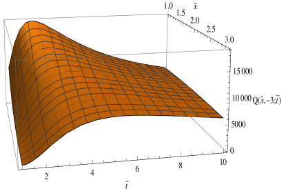
Figure 5: The three-dimensional profile of the particles density $Q(\widetilde{x},-3;\overline{t})$ to the right of the symmetric barrier.

One can see the nonmonotonic behavior of the density profile with time $\overline{t}$ for every fixed $\widetilde{x}$, especially pronounced near the right barrier boundary (near $\widetilde{x}=1$). This behavior, caused by the negative sources absorbing the particles (see Eq. (6)) and distributed according to the function (8) with $U>0$, $\Delta=0$, is quite different from the familiar ”free” diffusion in the absence of the potential ($U=0$, $\Delta=0$) which is shown in Fig. 6 for the same parameters as in Fig. 5.

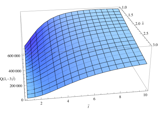
Figure 6: The spacetime density profile $Q(\widetilde{x},-3;\overline{t})$ for ”free” diffusion of the particles.

5 Summary

We have obtained the exact propagator $<x|\exp(-\alpha H)|x^{\prime}>$ ($H$ is the Hamiltonian for a particle moving in the presence of the asymmetric rectangular potential) resolving the parabolic-type partial differential equation. Having obtained the spacetime propagator for the one-dimensional time-dependent Schrödinger equation ($\alpha=it/\hbar$) with a rectangular well/barrier potential, we at the same time succeeded in finding a propagator for the Bloch equation ($\alpha=\beta$, $\beta=1/k_{B}t$) for the particle density matrix and for the diffusion-like equation ($\alpha=t$) by shifting from real to imaginary time ($t\rightarrow-i\hbar\beta$ and $t\rightarrow-it$, correspondingly). As an alternative to the conventional path integral approach to calculating the propagators, we use the multiple-scattering theory for the calculation of the energy-dependent Green function (a resolvent operator in (10)). The suggested approach is based on the possibility of introducing the effective potentials (see (14) and (15)) which are responsible for reflection from and transmission through the potential jumps making up the rectangular potential (8). It provides more of a non-classical picture of particle scattering at the considered potential as opposed to the conventional wave point of view.

The solution for the time-dependent Schrödinger equation describes the reflection from and transmission through the asymmetric rectangular potential as a function of time and thus allows for considering the non-classical counter-intuitive effects of particle reflection from a potential well and transmission through a potential barrier in a real situation when a particle is moving towards the potential (8) and then experiencing a scattering at the potential. These results are also relevant to the fundamental issues of measuring time in quantum mechanics such as the time-of-arrival (TOA), dwell time and tunneling time.

The obtained density matrix $\rho(x,x^{\prime};\beta)$ for a particle in a heat bath and under the influence of the potential (8) gives the probability density (diagonal matrix element) to find a particle in some spatial point and the quantum correlations (coherences) of different spatial states $|x>$ and $|x^{\prime}>$ provided by the nondiagonal matrix elements. The results for the density matrix are numerically visualized, which is enabled by the fact that they are expressed in terms of integrals of elementary functions.

The results of the solution of the diffusion-like equation, which can be interpreted (for the case of a potential barrier, $U>0$) as a diffusion with the negative sources distributed according to potential (8), also have been numerically evaluated. The corresponding figures demonstrate the difference between this ”diffusion with the holes” and ”free” diffusion in the absence of the potential (8).

It is also worth mentioning that all obtained results are also relevant to the properties of electrons in nanostructures important for spintronics devices because the potential (8) can be used for modeling potential profiles in such materials.

References

• [1] A.D. Baute, I.L. Egusquiza, and J.G. Muga, J. Phys. A: Math. Theor. 34, 42892001 (2001).
• [2] A.D. Baute, I.L. Egusquiza, and J.G. Muga, Int. J. Theor. Physics, Group Theory, and Nonlinear Optics 8, 1 (2002); (e-print arXiv:quant-ph/0007079).
• [3] J.G. Muga, R. Sala Mayato, and I.L. Egusquiza (ed), Time in Quantum Mechanics vol 1 (Lecture Notes in Physics vol 734) (Springer, Berlin, 2008). J.G. Muga, A. Ruschhaup, and A. del Campo (ed), Time in Quantum Mechanics vol 2 (Lecture Notes in Physics vol 789) (Springer, Berlin, 2009).
• [4] M.N. Baibich, J.M. Broto, A. Fert, F. Nguyen Van Dau, F. Petroff, P. Etienne, G. Creuzet, A. Friederich, and J. Chazelas, Phys. Rev. Lett. 61, 2472 (1988).
• [5] R. Julliere, Phys. Lett. A 54, 225 (1975); P. LeClair, J.S. Moodera, and R. Meservay, J. Appl. Phys. 76, 6546 (1994).
• [6] R.P. Feynman and A.R. Hibbs, Quantum Mechanics and Path Integrals (McGraw-Hill, New York, 1965).
• [7] M. Kac, Probability and Related Topics in Physical Sciencies (Lectures in Applied Mathematics vol 1) (Interscience Publishers, London, New York, 1958).
• [8] A.O. Barut and I.H. Duru, Phys. Rev. A 38, 5906 (1988).
• [9] L.S. Schulman, Phys. Rev. Lett. 49, 599 (1982).
• [10] T.O. de Carvalho, Phys. Rev. A 47, 2562 (1993).
• [11] J.M. Yearsley, J. Phys. A: Math. Theor. 41, 285301 (2008).
• [12] V.F. Los and A.V. Los, J. Phys. A: Math. Theor. 43, 055304 (2010).
• [13] V.F. Los and A.V. Los, J. Phys. A: Math. Theor. 44, 215301 (2011).
• [14] V.F. Los and M.V. Los, J. Phys. A: Math. Theor. 45, 095302 (2012).
• [15] J.G. Muga and C.R. Leavens, Phys. Rep. 338, (2000).
• [16] V.F. Los and M.V. Los, Theor. Math. Phys. 177, 1704 (2013).
• [17] E.N. Economou, Green’s Functions in Quantum Physics (Springer, Berlin, 1979).