Quantum entanglement and the Bell Matrix

Abstract.

We present a class of maximally entangled states generated by a high-dimensional generalisation of the cnot gate. The advantage of our constructive approach is the simple algebraic structure of both entangling operator and resulting entangled states. In order to show that the method can be applied to any dimension, we introduce new sufficient conditions for global and maximal entanglement with respect to Meyer and Wallach’s measure.

1. Introduction

Entanglement is a key feature of quantum mechanical systems with wide applications to the field of quantum information theory. The class of quantum processes relying on entangled states include quantum state teleportation [2], quantum error correction [3], quantum cryptography [11], and some quantum computational speedups [8]. Multi-qubit entangled states are regarded as a valuable resource for processing information: for instance, several authors applied multi-qubit entanglement (and related entangling procedures) to multi-agent generalizations of the quantum teleportation protocol introduced in the paper by Bennett, Brassard, Crèpeau, Jozsa, Peres, and Wootters [2] – see for instance [18]. Also, other classes of multi-qubit entangled states turned out to be suitable for superdense coding.

Applications to quantum information theory motivated the search for the mathematical characterisations of multi-particle entanglement and for highly entangled quantum states. The approaches to this problem include an analytical classifications of entangled states [4, 17], numerical optimisation techniques [5], and geometric characterisations [10].

Here we present a class of maximally entangled states, that we call general Bell states or $2^{n}$-dimensional Bell states, generated by an arbitrarily high-dimensional generalisation of the cnot gate. The advantage of our approach is the simple algebraic structure of both entangling gates and resulting states. In order to show the full generality of the method, we prove new sufficient conditions for both global entanglement and maximal entanglement (with respect to Meyer and Wallach’s measure, see Equation (1)): being based on the expectation value of an explicitly given operator, these criteria feature a simple formulation, scalability and observability.

In [13] Osterloh and Siewert propose a general method to construct new classes of entanglement measures based on suitable products and combinations of Pauli’s matrices. Inspired by this approach, as well as by the multi-qubit concurrence proposed in [1] and by the relation between antilinear operators and concurrence [16], in what follows, we introduce a particular antilinear operator (Definition 4) and we use its expectation value as an entanglement criterion (Proposition 6) for general Bell states. In Proposition 9, we show that such an operator turns out to be related to Meyer and Wallach’s (MW) measure [12] and we employ this relation to show that the general Bell states are maximally entangled with respect to this measure – Theorem 16.

To the best of our knowledge, an univoque and commonly accepted notion of entanglement measure in high-dimensional systems has not yet been introduced. Several proposals in the literature try to capture distinct aspects of a maximally entangled state. For instance, the Schmidt decomposition, see [7], induces a measure related to the minimum number of terms in the product expansion of a state, while the fully entangled fraction measures the ability of a state to perform tasks related to quantum computing, such as teleportation and dense coding [9].

Throughout this paper, we focus on MW measure [12]. This measure interprets the global entanglement as the average bipartite entanglement of every qubit with respect to the rest of the system. It has thus the advantage of a simple physical meaning as well as a simple formulation, introduced in [6]:

(1) $$Q(|\psi\rangle):=2\left(1-\frac{1}{n}\sum_{j=1}^{n}Tr[\rho_{j}^{2}]\right)$$

where $n$ is the number of qubits of the system, $\rho_{j,\psi}$ is the density matrix obtained by tracing out the $j$-th qubit of the state $|\psi\rangle$ and $Tr[\cdot]$ represents the trace operator.

The main result we present here is a sufficient condition on multi-qubit states to be maximally entangled (with respect to MW measure) and, as mentioned above, we establish this result in order to show that a set of states generalising Bell states have maximal MW measure.

The paper is organised as follows. In Section 2 we show sufficient conditions for global entanglement and for the maximality of the MW measure of a state in a multi-qubit system. In Section 3 we propose a generalisation of the cnot gate to multi-qubit systems a related class of states, that we call $2^{n}$-dimensional Bell states. By applying the criteria introduced in Section 2, we are able to show that these generalisations of Bell states are maximally entangled with respect to MW measure. Some possible extensions of this approach are illustrated in Section 3.1.

2. An entanglement criterion

First of all we give the formal definition of globally entangled state.

Definition 1.

A state $|\psi\rangle$ is globally entangled if for any $|\phi_{1}\rangle$ and $|\phi_{2}\rangle$ we have $|\psi\rangle\neq|\phi_{1}\rangle\otimes|\phi_{2}\rangle$.

Remark 2.

Throughout this paper we consider elements of Hilbert spaces $|\psi\rangle\in\mathbb{C}^{2^{n}}$ which are pure quantum states, i.e., they are complex vectors of unit Euclidean norm: $|\psi\rangle=(\psi_{1},\dots,\psi_{2^{n}})$ and $\sum_{j=1}^{2^{n}}|\psi_{j}|^{2}=1$; for brevity we refer to them simply as “states”.

Notation 3.

We use the symbol $I_{2^{n}}$ to denote the $2^{n}$-dimensional identity matrix:

$$I_{2^{n}}:=\underbrace{I_{2}\otimes\dots\otimes I_{2}}_{n-\text{times}}.$$

being $I_{2^{n}}=(1)$ if $n=0$.

The expectation value of the operator $A$ in the state $\psi$ is denoted by

$$\langle A\rangle_{\psi}:=\langle\psi|A|\psi\rangle.$$

Moreover we denote by $\sigma_{y}$ the Pauli matrix

$$\begin{pmatrix}0&-i\\ i&0\end{pmatrix}.$$

We introduce the following two operators, they are used to define the particular antilinear operator we apply to states constructed with algorithm in Section 3 in order to prove they are entangled states.

Definition 4.

Let us denote by $\mathcal{F}:\mathbb{C}^{2^{n}}\to\mathbb{C}$ the function which associates to a state $|\psi\rangle$ the expectation value of the operator $M_{2^{n}}K_{2^{n}}$ in the state $|\psi\rangle$, namely:

(2) $$\mathcal{F}(|\psi\rangle):=\langle M_{2^{n}}K_{2^{n}}\rangle_{\psi}$$

where $M_{2^{n}}:=\sigma_{y}\otimes I_{2^{n-2}}\otimes\sigma_{y}$ and $K_{2^{n}}$ is the conjugation operator.

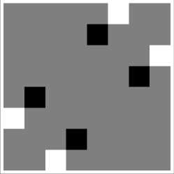
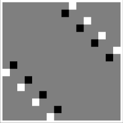
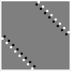
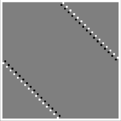
Figure 1. We show in this picture the matrices $M_{2^{n}}$ for $n=2,\dots,7$. Entries $0$ are shown in grey color, entries $+1$ by black color and entries $-1$ by white color.

Note that

$$\mathcal{F}(|\psi\rangle):=\langle M_{2^{n}}K_{2^{n}}\rangle_{\psi}=\langle\psi|M_{2^{n}}K_{2^{n}}|\psi\rangle=\langle\psi|M_{2^{n}}|\bar{\psi}\rangle$$

where $|\bar{\psi}\rangle$ denotes the complex conjugate of $|\psi\rangle$.

Example 5.

We explicitly compute $M_{4}$:

$$M_{4} :=\sigma_{y}\otimes I_{2^{2-2}}\otimes\sigma_{y}=\sigma_{y}\otimes(1)\otimes\sigma_{y}=$$

$$=\sigma_{y}\otimes\sigma_{y}=\begin{pmatrix}0&-i\\ i&0\end{pmatrix}\otimes\sigma_{y}=\begin{pmatrix}0&-i\sigma_{y}\\ i\sigma_{y}&0\end{pmatrix}=\begin{pmatrix}0&0&0&-1\\ 0&0&1&0\\ 0&1&0&0\\ -1&0&0&0\\ \end{pmatrix}$$

For a representation of matrices $M_{2^{n}}$ with $n\geq 2$ see Figure 1.

We now show that $M_{2^{n}}K_{2^{n}}$ has zero expectation value on product states.

Proposition 6.

If $|\psi\rangle$ is an unentangled state then $\mathcal{F}(|\psi\rangle)=0$.

Proof.

Let $n\geq 1$, $|\psi\rangle\in\mathbb{C}^{2^{n}}$, $|\phi_{1}\rangle\in\mathbb{C}^{2^{n_{1}}}$, $|\phi_{2}\rangle\in\mathbb{C}^{2^{n_{2}}}$, $n_{1}+n_{2}=n$ and assume $|\psi\rangle=|\phi_{1}\rangle\otimes|\phi_{2}\rangle$. Also let $|\bar{\phi}_{1}\rangle=(a,b)\in\mathbb{C}^{2^{n_{1}}}$ defined by $a,b\in\mathbb{C}^{2^{n_{1}-1}}$, two half vectors of its coordinates in the standard basis. One has

$$(\sigma_{y}\otimes I_{2^{n_{1}-1}})(a,b)=-i(b,-a).$$

Consequently

(3) $$\langle\phi_{1}|\sigma_{y}\otimes I_{2^{n_{1}-1}}|\bar{\phi}_{1}\rangle=(a,b)^{\mbox{\scriptsize\sc t}}(\sigma_{y}\otimes I_{2^{n_{1}-1}})(a,b)=-ia\cdot b+ib\cdot a=0.$$

Similarly, if $|\bar{\phi}_{2}\rangle=(y_{1},\dots,y_{2^{n_{2}}})$ then

$$(I_{2^{n_{2}-1}}\otimes\sigma_{y})|\bar{\phi}_{2}\rangle =(I_{2^{n_{2}-1}}\otimes\sigma_{y})(y_{1},\dots,y_{2^{n}})$$

$$=-i(y_{2},-y_{1},y_{3},-y_{4},\dots,y_{2^{n_{2}}},-y_{2^{n_{2}}-1})$$

thus

(4) $$\begin{split}\langle\phi_{2}|I_{2^{n_{2}-1}}&\otimes\sigma_{y}|\bar{\phi}_{2}\rangle=(y_{1},\dots,y_{2^{n_{2}}})^{\mbox{\scriptsize\sc t}}(I_{2^{n_{2}-1}}\otimes\sigma_{y})(y_{1},\dots,y_{2^{n_{2}}})\\ &=-i(y_{1},\dots,y_{2^{n_{2}}})^{\mbox{\scriptsize\sc t}}(y_{2},-y_{1},y_{3},-y_{4},\dots,y_{2^{n_{2}}},-y_{2^{n_{2}}-1})=0.\end{split}$$

By equalities (3) and (4) one finally has

$$\mathcal{F}(|\psi\rangle) =\langle\psi|M_{2^{n}}|\bar{\psi}\rangle=\langle\phi_{1}\otimes\phi_{2}|\sigma_{y}\otimes I_{2^{n-2}}\otimes\sigma_{y}|\bar{\phi}_{1}\otimes\bar{\phi}_{2}\rangle$$

$$=\langle\phi_{1}\otimes\phi_{2}|\sigma_{y}\otimes I_{2^{n_{1}-1}}\otimes I_{2^{n_{2}-1}}\otimes\sigma_{y}|\bar{\phi}_{1}\otimes\bar{\phi}_{2}\rangle$$

$$=\langle\phi_{1}|\sigma_{y}\otimes I_{2^{n_{1}-1}}|\bar{\phi}_{1}\rangle\langle\phi_{2}|I_{2^{n_{2}-1}}\otimes\sigma_{y}|\bar{\phi}_{2}\rangle=0.$$

∎

Next result shows that $\mathcal{F}$ also provides a sufficient condition for maximal entanglement. It is useful to recall the following

Definition 7 (Schimdt decomposition).

Let $n_{1},n_{2}\in\mathbb{N}$ such that $n_{1}+n_{2}=n$ and let $A=\mathbb{C}^{2^{n_{1}}}$ and $B=\mathbb{C}^{2^{n_{2}}}$ so that $\mathbb{C}^{2^{n}}=A\otimes B$. Then any state $|\psi\rangle\in\mathbb{C}^{2^{n}}$ can be written in the form

$$|\psi\rangle=\sum_{k=1}^{K}c_{k}|\phi_{k}^{A}\rangle\otimes|\phi_{k}^{B}\rangle$$

where $K=\min\{dim(A),dim(B)\}=\min\{2^{n_{1}},2^{n_{2}}\}$, $c_{k}\geq 0$ and $\{|\phi_{k}^{A}\rangle\}$, $\{|\phi^{B}_{k}\rangle\}$ are two orthonormal subsets of $A$ and $B$, respectively [14]. This decomposition takes the name of Schmidt decomposition.

Remark 8.

Consider the decomposition $\mathbb{C}^{2^{n}}=A\otimes B$ and let $\rho_{A,\psi}$ be the density operator of the state $|\psi\rangle$ on the subsystem $A$. Then the set of the positive eigenvalues of $\rho_{A,\psi}$ coincides with the set $\{c_{k}^{2}\mid c_{k}>0\}$ of positive squared coefficients of Schmidt decomposition of the state $|\psi\rangle$ with respect to the decomposition $\mathbb{C}^{2^{n}}=A\otimes B$ – see for instance [15]. As a consequence, $Tr[\rho_{A,\psi}]=\sum_{k=1}^{K}c_{k}^{2}=1$ and $Tr[\rho^{2}_{A,\psi}]=\sum_{k=1}^{K}c_{k}^{4}$.

Proposition 9.

If $|\mathcal{F}(|\psi\rangle)|=1$ then $|\psi\rangle$ is maximally entangled with respect to MW measure.

Proof.

First of all we notice that

1. If $|\phi\rangle\in\mathbb{C}^{2}$ then $\langle\phi|\sigma_{y}|\bar{\phi}\rangle=0$;

2. If $\{|\phi_{1}\rangle,|\phi_{2}\rangle\}$ is an orthonormal base of $\mathbb{C}^{2}$ then $|\langle\phi_{1}|\sigma_{y}|\bar{\phi}_{2}\rangle|=1$ and

   $$\langle\phi_{1}|\sigma_{y}|\bar{\phi}_{2}\rangle=-\langle\phi_{2}|\sigma_{y}|\bar{\phi}_{1}\rangle$$

3. For all $|\xi_{1}\rangle,|\xi_{2}\rangle\in\mathbb{C}^{2^{n-1}}$ one has

   $$|\langle\xi_{1}|I_{2^{n-2}}\otimes\sigma_{y}|\bar{\xi}_{2}\rangle|\leq 1;$$

   and

   $$\langle\xi_{1}|I_{2^{n-2}}\otimes\sigma_{y}\bar{\xi}_{2}\rangle=-\langle\xi_{2}|I_{2^{n-2}}\otimes\sigma_{y}|\bar{\xi}_{1}\rangle.$$

Also remark that the Schmidt decomposition of $|\psi\rangle$ with respect the decomposition that singles out a generic qubit of the system reads:

$$|\psi\rangle=\sum_{k=1}^{2}c_{k}|\phi_{k}\rangle\otimes|\xi_{k}\rangle$$

for some $c_{1},c_{2}\geq 0$ such that $c_{1}^{2}+c_{2}^{2}=1$, some orthonormal base $\{|\phi_{1}\rangle,|\phi_{2}\rangle\}$ of $\mathbb{C}^{2}$ and some orthonormal subset $\{|\xi_{1}\rangle,|\xi_{2}\rangle\}$ of $\mathbb{C}^{2^{n-1}}$.

In view of (a)-(c), we then have

$$|\mathcal{F}(|\psi\rangle)| =|\sum_{k,h=1}^{2}c_{k}c_{h}\langle\phi_{k}|\sigma_{y}|\phi_{h}\rangle\langle\xi_{k}|I_{2^{n-2}}\otimes\sigma_{y}|\bar{\xi}_{h}\rangle|$$

$$=|2c_{1}c_{2}\langle\xi_{1}|I_{2^{n-2}}\otimes\sigma_{y}|\bar{\xi}_{2}\rangle|\leq|2c_{1}c_{2}|$$

On the other hand $|2c_{1}c_{2}|\leq 1$ for all $c_{1},c_{2}\in\mathbb{R}$ such that $c_{1}^{2}+c_{2}^{2}=1$, and the maximum $|2c_{1}c_{2}|=1$ is attained at the points satisfying $c_{1}^{2}=c_{2}^{2}=1/2$. Therefore we may conclude that if $|\mathcal{F}(|\psi\rangle)|=1$ then $c_{1}^{2}=c_{2}^{2}=1/2$. Since this argument holds for any qubit, we have that

$$Tr[\rho_{j,\psi}^{2}]=c_{1}^{4}+c_{2}^{4}=\frac{1}{2}\quad\text{ for all $j=1,\dots,n$}$$

see also Remark 8. Consequently,

$$Q(|\psi\rangle)=2\left(1-\frac{1}{n}\sum_{j=1}^{n}Tr[\rho_{j,\psi}^{2}]\right)=1.$$

∎

Above results relate the value of $|\mathcal{F}(|\psi\rangle)|$ to a measure of entanglement of the state $|\psi\rangle$. In particular if $|\mathcal{F}(|\psi\rangle)|$ is minimal, i.e., $|\mathcal{F}(|\psi\rangle)|=0$, then $|\psi\rangle$ is not entangled while if $|\mathcal{F}(|\psi\rangle)|$ is maximal, i.e., $|\mathcal{F}(|\psi\rangle)|=1$ then $|\psi\rangle$ is maximally entangled. However the condition $|\mathcal{F}(|\psi\rangle)|=0$ (respectively $|\mathcal{F}(|\psi\rangle)|=1$) is a necessary but not sufficient condition to have $|\psi\rangle$ unentangled (resp. maximally entangled). Indeed, consider the Greenberger-Horne-Zeilinger state

$$|GHZ_{n}\rangle:=\frac{1}{\sqrt{2}}(|0_{n}\rangle+|1_{n}\rangle).$$

For all $n\geq 2$, the state $|GHZ_{n}\rangle$ is globally entangled state and yet, for $n\geq 3$, $\mathcal{F}(|GHZ_{n}\rangle)=0$: this implies that, in general, the inverse implication of Proposition 6 (that is, $\mathcal{F}(|\psi\rangle)=0$ implies $|\psi\rangle$ is unentangled) is not true. Furthermore, for all $n\geq 2$, the state $|GHZ_{n}\rangle$ is maximally entangled with respect to MW measure and $\mathcal{F}(|\psi\rangle)\not=1$, thus also the inverse implication of Proposition 9 (that is, $\mathcal{F}(|\psi\rangle)=1$ implies $|\psi\rangle$ is maximally entangled) in general is not true.

3. $n$-qubit entanglement algorithm

In this section we introduce a generalisation of the cnot gate and we show that the resulting Bell state are fully entangled.

Figure 2. Bell Circuit: entanglement of two elements of the canonical basis $|0\rangle$ and $|1\rangle$

To this end we adopt the following notations:

Notation 10.

We use $H_{2}:=\frac{1}{\sqrt{2}}\begin{pmatrix}1&1\\ 1&-1\end{pmatrix}$ is the Hadamard matrix and

$$H_{2^{n}}:=\underbrace{H_{2}\otimes\dots\otimes H_{2}}_{n\text{ times}}$$

is its $2^{n}$-dimensional generalisation, i.e., the $2^{n}$-dimensional Walsh matrix. We use the symbols $\sigma_{x},\sigma_{y}$ and $\sigma_{z}$ to denote Pauli’s matrices

$$\sigma_{x}=\begin{pmatrix}0&1\\ 1&0\end{pmatrix},\qquad\sigma_{y}=\begin{pmatrix}0&-i\\ i&0\end{pmatrix},\qquad\sigma_{z}=\begin{pmatrix}1&0\\ 0&-1\end{pmatrix}.$$

We finally consider the orthogonal projectors

$$L:=\left(\begin{array}[]{cc}1&0\\ 0&0\end{array}\right),\qquad R:=\left(\begin{array}[]{cc}0&0\\ 0&1\end{array}\right).$$

In view of above notation, we remark that the cnot gate satisfies the equality

$$\text{{cnot}}:=\begin{pmatrix}1&0&0&0\\ 0&1&0&0\\ 0&0&0&1\\ 0&0&1&0\\ \end{pmatrix}=L\otimes I_{2}+R\otimes\sigma_{x}$$

while the columns of the matrix

$$B_{4}:=\frac{1}{\sqrt{2}}\begin{pmatrix}1&0&1&0\\ 0&1&0&1\\ 0&1&0&-1\\ 1&0&-1&0\\ \end{pmatrix}=\text{{cnot}}(H_{2}\otimes I_{2})$$

are the coordinate vectors of the Bell states in the standard base. We extend the above definitions of cnot and of $B_{2}$ to an arbitrary number of qubits as follows

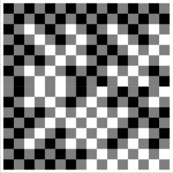
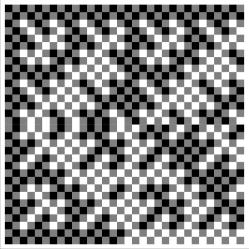
Figure 3. We show in this picture Bell matrices $B_{2^{n}}$ for $n=2,\dots,7$. Entries $0$ are shown in grey color, entries $+1$ by black color and entries $-1$ by white color.

Definition 11.

For $n\geq 2$ we set

(5) $$\text{{cnot}}_{2^{n}}:=L\otimes I_{2^{n-1}}+R\otimes\underbrace{\sigma_{x}\otimes\dots\otimes\sigma_{x}}_{n-1\text{ times}}$$

and

(6) $$B_{2^{n}}:=\text{{cnot}}_{2^{n}}(H_{2^{n-1}}\otimes I_{2}).$$

We define $2^{n}$-dimensional Bell state any state

$$|b_{k}\rangle:=B_{2^{n}}|k\rangle$$

where $k=0,\dots,2^{n}-1$ and $|k\rangle$ is the $k$-th element of the standard base of $\mathbb{C}^{2^{n}}$.

In what follows we show that the $2^{n}$-dimensional Bell states are maximally entangled with respect to MW measure. We introduce the matrix

(7) $$L_{2^{n}}:=B_{2^{n}}^{\dagger}M_{2^{n}}B_{2^{n}},$$

whose relevance in our investigation is motivated by the following

Lemma 12.

If $|\langle\phi|L_{2^{n}}|\bar{\phi}\rangle|=1$ and if $|\psi\rangle=B_{2^{n}}|\phi\rangle$ then $|\psi\rangle$ is maximally entangled with respect to the MW measure.

In particular, if $|\langle k|L_{2^{n}}|\bar{k}\rangle|=1$, where $|k\rangle$ is the $k$-th element of the standard base, then the $k$-th Bell state is maximally entangled with respect to the MW measure.

Proof.

By the definition of $L_{2^{n}}$ and by the assumption $|\psi\rangle=B_{2^{n}}|\phi\rangle$ one has

$$|\langle\phi|L_{2^{n}}|\bar{\phi}\rangle| =|\langle\phi|B_{2^{n}}^{\dagger}M_{2^{n}}B_{2^{n}}|\bar{\phi}\rangle|$$

$$=|\langle B_{2^{n}}\phi|M_{2^{n}}|\overline{(B_{2^{n}}|\phi)}\rangle|=|\langle\psi|M_{2^{n}}|\bar{\psi})\rangle|=|\mathcal{F}(|\psi\rangle)|.$$

The first part of the claim hence follows by Proposition 9.

The second part of the claim readily follows by applying above reasoning to $|\phi\rangle=|k\rangle$ and by the definition of $2^{n}$-dimensional Bell state. ∎

Remark 13.

There exist states $\phi$ which not satisfy $|\langle\phi|L_{2^{n}}|\bar{\phi}\rangle|=1$ and such that $B_{2^{n}}|\phi\rangle$ is maximally entangled, an example of this phenomenon is given by the state $\phi=B^{-1}_{2^{n}}|GHZ_{n}\rangle$.

Next result gives a closed formula for $L_{2^{n}}$ and relates its diagonal elements to the Thue-Morse sequence, that is the binary sequence $(\tau_{i})$ defined by the recursive relation

$$\tau_{1}:=0$$

$$\tau_{2n}:=1-\tau_{n}$$

$$\tau_{2n-1}:=\tau_{n}$$

for all positive integers $n$. We notice that for all $n\geq 1$

(8) $$\tau_{2^{n}+i}=1-\tau_{i}\quad\text{for all $i=1,\dots,2^{n}$}.$$

Remark 14.

Equality (8) characterises the Thue-Morse sequence via bitwise negation, indeed it states that every initial block of length $2^{n}$, i.e, $\tau_{1},\dots,\tau_{2^{n}}$, is followed by a block of equal length that is its bitwise negation, i.e., $\tau_{2^{n}+1}=1-\tau_{1},\dots,\tau_{2^{n+1}}=1-\tau_{2^{n}}$. This can be proved by an inductive argument, indeed the case $n=1$ follows by a direct computation and, assuming (8) as inductive hypothesis, one readily gets the inductive step

$$\tau_{2^{n+1}+i}=\begin{cases}\tau_{2(2^{n}+i/2)}=1-\tau_{2^{n}+i/2}=1-\tau_{i/2}=1-\tau_{i}&\quad\text{if $i$ is even;}\\ \tau_{2(2^{n}+i/2)}=\tau_{2^{n}+(i+1)/2}=1-\tau_{(i+1)/2}=1-\tau_{i}&\quad\text{if $i$ is odd.}\end{cases}$$

Lemma 15.

For all $n\geq 2$

(9) $$L_{2^{n}}=-\underbrace{\sigma_{z}\otimes\dots\otimes\sigma_{z}}_{n\text{ times}}.$$

Moreover $L_{2^{n}}$ is a diagonal matrix whose diagonal elements $L_{2^{n},i}$, ${i=1,\dots,2^{n}}$, satisfy

(10) $$L_{2^{n},i}=2\tau_{i}-1,\qquad\text{for all $n=1,\dots,2^{n}$},$$

where $(\tau_{i})$ is the Thue-Morse sequence.

Proof.

In order to prove (9), we recall the definition of $L_{2^{n}}$ in Equation (7)

(11) $$\begin{split}L_{2^{n}}=&B^{\dagger}_{2^{n}}M_{2^{n}}B_{2^{n}}\\ =&(LH_{2})^{\dagger}\sigma_{y}RH_{2}\otimes\underbrace{(H_{2}^{\dagger}\sigma_{x}H_{2})\otimes\dots\otimes(H_{2}^{\dagger}\sigma_{x}H_{2})}_{n-1\text{ times}}\otimes\sigma_{y}\sigma_{x}+\\ &+(RH_{2})^{\dagger}\sigma_{y}LH_{2}\otimes\underbrace{((\sigma_{x}H_{2})^{\dagger}H_{2})\otimes\dots\otimes((\sigma_{x}H_{2})^{\dagger}H_{2})}_{n-1\text{ times}}\otimes\sigma_{x}^{\dagger}\sigma_{y}\end{split}$$

the second equality is obtained by applying Definition 11, Equations (5) and (6) where $B_{2^{n}}$ is given in terms of $\text{{cnot}}_{2^{n}}$, namely

$$B_{2^{n}}=(LH_{2})\otimes\underbrace{H_{2}\otimes\dots\otimes H_{2}}_{(n-1)\text{ times}}+(RH_{2})\otimes\underbrace{\sigma_{x}H_{2}\otimes\dots\otimes\sigma_{x}H_{2}}_{(n-1)\text{ times}}$$

and by applying $L^{\dagger}\sigma_{y}L=R^{\dagger}\sigma_{y}R=0$. By a direct computation

$$(RH_{2})^{\dagger}\sigma_{y}LH_{2}=((LH_{2})^{\dagger}\sigma_{y}RH_{2})^{\dagger}=-\frac{i}{2}\begin{pmatrix}-1&1\\ -1&1\\ \end{pmatrix}\quad\text{and}\quad\sigma_{x}^{\dagger}\sigma_{y}=(\sigma_{y}\sigma_{x})^{\dagger}=i\sigma_{z}.$$

By plugging above relations in (11) we obtain the first part of the claim, indeed

$$L_{2^{n}}= \frac{i}{2}\begin{pmatrix}-1&1\\ -1&1\\ \end{pmatrix}\otimes\underbrace{\sigma_{z}\otimes\dots\otimes\sigma_{z}}_{n-2\text{ times}}\otimes(-i\sigma_{z})-\frac{i}{2}\begin{pmatrix}-1&-1\\ 1&1\\ \end{pmatrix}\otimes\underbrace{\sigma_{z}\otimes\dots\otimes\sigma_{z}}_{n-2\text{ times}}\otimes i\sigma_{z}$$

$$= \frac{1}{2}\begin{pmatrix}-1&1\\ -1&1\\ \end{pmatrix}\otimes\underbrace{\sigma_{z}\otimes\dots\otimes\sigma_{z}}_{n-1\text{ times}}+\frac{1}{2}\begin{pmatrix}-1&-1\\ 1&1\\ \end{pmatrix}\otimes\underbrace{\sigma_{z}\otimes\dots\otimes\sigma_{z}}_{n-1\text{ times}}$$

$$= -\underbrace{\sigma_{z}\otimes\dots\otimes\sigma_{z}}_{n\text{ times}}.$$

Now, above equality implies

(12) $$L_{2^{n}}=\sigma_{z}\otimes L_{2^{n-1}}$$

and, by an inductive argument, that $L_{2^{n}}$ is a diagonal matrix.

Finally we prove (10) by induction on $n$. The base of induction, i.e. the case $n=1$, readily follows by $L_{2}=\sigma_{z}$ and by the definition of $\tau_{1}$ and of $\tau_{2}$. Now we prove the inductive step, i.e., we assume (10) as inductive hypothesis and we show

(13) $$L_{2^{n+1},i}=2\tau_{i}-1,\qquad\text{for all $i=1,\dots,2^{n+1}$},$$

By (12) we have $L_{2^{n+1}}=\sigma_{z}\otimes L_{2^{n}}$ and, consequently,

$$L_{2^{n+1},i}=\begin{cases}L_{2^{n},i}\quad&\text{if }i\leq 2^{n}\\ -L_{2^{n},i-2^{n}}\quad&\text{otherwise}.\end{cases}.$$

This, together with (8), implies (13), indeed we have

$$L_{2^{n+1},i}=L_{2^{n},i}=2\tau_{i}-1$$

$$L_{2^{n+1},2^{n}+i}=-L_{2^{n},i}=1-2\tau_{i}=2\tau_{2^{n}+i}-1$$

for all $i=1,\dots,2^{n}$ and this completes the proof. ∎

Theorem 16.

The $2^{n}$-dimensional Bell states are maximally entangled with respect to MW measure.

Proof.

By Lemma 15, $L_{2^{n}}$ is a diagonal matrix with $1$ or $-1$ as diagonal elements then $|\langle k|L_{2^{n}}|\bar{k}\rangle|=1$ for all $k=0,\dots,2^{n}-1$ and this, together with Lemma 12, implies the claim. ∎

3.1. Some remarks on an entanglement criterion

Lemma 12 provides a maximal entanglement criterion that can be rephrased as follows “If $|\langle\phi|L_{2^{n}}|\bar{\phi}\rangle|=1$ then $B_{2^{n}}|\phi\rangle$ is maximally entangled”. Then one may ask how is made the space of states satisfying this condition. Lemma 15 provides some answers to this question. Indeed we already used in the proof of Theorem 16 the fact that $|\langle k|L_{2^{n}}|k\rangle|=1$, if $|k\rangle$ is an element of the canonical base. Next result investigates this property in the larger class of states whose coordinates in the standard base are real valued.

Proposition 17.

Let $(\tau_{i})$ be the Thue-Morse sequence and let $o_{i}$ and $e_{i}$ be the index sequences such that $\tau_{o_{i}}=1$ and $\tau_{e_{i}}=0$ for all $i\in\mathbb{N}$. Then for all $x\in\mathbb{R}^{2^{n}}$ with $|x|=1$, one has $|x^{\mbox{\scriptsize\sc t}}L_{2^{n}}x|=1$ if and only if either $x_{e_{i}}=0$ for all $i=1,\dots,2^{n-1}$ or $x_{o_{i}}=0$ for all $i=1,\dots,2^{n-1}$.

Proof.

Let $x=(x_{1},\dots,x_{2^{n}})\in\mathbb{R}^{2^{n}}$ with $|x|=1$. Since $x$ is real valued then $|x_{i}|^{2}=x_{i}^{2}$ for all $i=1,\ldots,2^{n}$ and $\sum_{i=1}^{2^{n}}x^{2}_{i}=|x|^{2}$. On the other hand $|x^{\mbox{\scriptsize\sc t}}L_{2^{n}}x|=|\sum_{i=1}^{2^{n}}\tau_{i}x^{2}_{i}|=1$ if and only if either $\sum_{i=1}^{2^{n}}L_{2^{n},i}x^{2}_{i}=1$ or $\sum_{i=1}^{2^{n}}L_{2^{n},i}x^{2}_{i}=-1$, where $L_{2^{n},i}$ is the $i$-th diagonal element of $L_{2^{n}}$. Since $|x|=1$, the former case is equivalent to $\sum_{i=1}^{2^{n}}L_{2^{n},i}x^{2}_{i}=\sum_{i=1}^{2^{n}}x^{2}_{i}$ and, this, together with the equality $L_{2^{n},i}=2\tau_{i}-1$ proved in Lemma 15, implies

$$0=\sum_{i=1}^{2^{n}}(L_{2^{n},i}-1)x^{2}_{i}=\sum_{i=1}^{2^{n}}(2\tau_{i}-2)x^{2}_{i}=-2\sum_{i=1}^{2^{n-1}}x^{2}_{e_{i}}.$$

Above equality holds if and only if $x_{e_{i}}=0$ for all $i=1,\dots,2^{n-1}$. It follows by a similar argument that $\sum_{i=1}^{2^{n}}\tau_{i}x^{2}_{i}=-1$ is equivalent to $x_{o_{i}}=0$ for all $i=1,\dots,2^{n-1}$ and this completes the proof. ∎

Remark 18.

The index sequences $e_{i}$ and $o_{i}$ defined in above Proposition are called Conway’s odious and evil numbers.

4. Conclusions

We proposed a family of unitary transformations generalising the cnot gate to an arbitrary number of qubits. We showed that a circuit composed by Walsh matrix and our general cnot gate yields a maximally entangled (with respect to MW measure) set of states, that we called generalised Bell states. In order to prove the validity of the method, we developed ad hoc entanglement criteria based on the definition of a suitable antilinear operator. The paper also contains a preliminary theoretical investigation of such operator, which turned out to be related with the celebrated Thue-Morse sequence.

Results in the present paper open the way to further investigations in several directions. For instance, it could be interesting to extend the method to general controlled unitary operations. Also, a deeper investigation of antilinear operators with zero expectation value on product states could represent a step towards an algebraic characterisation of the states with maximal MW measure. Finally it could be interesting to better understand the intriguing relation between states with maximal MW measure and the Thue-Morse sequence.

References

• [1] Yacob Ben-Aryeh. The use of Braid operators for implementing entangled large $n$-qubits Bell states ($n>2$). arXiv preprint arXiv:1403.2524, 2014.
• [2] Charles H. Bennett, Gilles Brassard, Claude Crépeau, Richard Jozsa, Asher Peres, and William K Wootters. Teleporting an unknown quantum state via dual classical and Einstein-Podolsky-Rosen channels. Physical review letters, 70(13):1895–1899, 1993.
• [3] Charles H. Bennett, David P. DiVincenzo, John A. Smolin, and William K. Wootters. Mixed-state entanglement and quantum error correction. Physical Review A, 54(5):3824, 1996.
• [4] Charles H. Bennett, Sandu Popescu, Daniel Rohrlich, John A. Smolin, and Ashish V. Thapliyal. Exact and asymptotic measures of multipartite pure-state entanglement. Physical Review A, 63(1):012307, 2000.
• [5] A Borras, AR Plastino, Josep Batle, Claudia Zander, Montserrat Casas, and A Plastino. Multiqubit systems: highly entangled states and entanglement distribution. Journal of Physics A: Mathematical and Theoretical, 40(44):13407, 2007.
• [6] Gavin K. Brennen. An observable measure of entanglement for pure states of multi-qubit systems. Quantum Information and Computation, 3(6):619–626, 2003.
• [7] Jens Eisert and Hans J. Briegel. Schmidt measure as a tool for quantifying multiparticle entanglement. Physical Review A, 64(2):022306, 2001.
• [8] Artur Ekert and Richard Jozsa. Quantum algorithms: entanglement-enhanced information processing. Philosophica transactions – Royal society of London Serie A: mathematical physical and engineering sciences, 356(1473):1769–1781, 1998.
• [9] John P. Grondalski, David M. Etlinger, and Daniel F. V. James. The fully entangled fraction as an inclusive measure of entanglement applications. 300(6):573–580, 2002.
• [10] Hoshang Heydari. Topological quantum gate entanglers for a multi-qubit state. Journal of Physics A: Mathematical and Theoretical, 40(32):9877, 2007.
• [11] Thomas Jennewein, Christoph Simon, Gregor Weihs, Harald Weinfurter, and Anton Zeilinger. Quantum cryptography with entangled photons. Physical Review Letters, 84(20):4729, 2000.
• [12] David A. Meyer and Nolan R. Wallach. Global entanglement in multiparticle systems. J. Math. Phys., 43(9):4273–4278, 2002. Quantum information theory.
• [13] Andreas Osterloh and Jens Siewert. Constructing $n$-qubit entanglement monotones from antilinear operators. Phys. Rev. A, 72:012337, Jul 2005.
• [14] Anirban Pathak. Elements of quantum computation and quantum communication. Taylor & Francis, 2013.
• [15] Eleanor G. Rieffel and Wolfgang H. Polak. Quantum computing: A gentle introduction. MIT Press, 2011.
• [16] Armin Uhlmann. Fidelity and concurrence of conjugated states. Phys. Rev. A, 62:032307, Aug 2000.
• [17] Guifré Vidal. Entanglement monotones. Journal of Modern Optics, 47(2-3):355–376, 2000.
• [18] Chui-Ping Yang, Shih-I Chu, and Siyuan Han. Efficient many-party controlled teleportation of multiqubit quantum information via entanglement. Physical Review A, 70(2):022329, 2004.