$\bm{Q}$-colourings of the triangular lattice:
Exact exponents and conformal field theory

Abstract

We revisit the problem of $Q$-colourings of the triangular lattice using a mapping onto an integrable spin-one model, which can be solved exactly using Bethe Ansatz techniques. In particular we focus on the low-energy excitations above the eigenlevel $g_{2}$, which was shown by Baxter to dominate the transfer matrix spectrum in the Fortuin-Kasteleyn (chromatic polynomial) representation for $Q_{0}\leq Q\leq 4$, where $Q_{0}=3.819\,671\cdots$. We argue that $g_{2}$ and its scaling levels define a conformally invariant theory, the so-called regime IV, which provides the actual description of the (analytically continued) colouring problem within a much wider range, namely $Q\in(2,4]$. The corresponding conformal field theory is identified and the exact critical exponents are derived. We discuss their implications for the phase diagram of the antiferromagnetic triangular-lattice Potts model at non-zero temperature. Finally, we relate our results to recent observations in the field of spin-one anyonic chains.

, ,

1 Introduction

The four-colour problem is probably the best known problem of graph theory, and has fascinated generations of mathematicians and laymen since it was first stated in a letter from Augustus de Morgan to Sir William Rowan Hamilton dated 23 October 1852. The suspense was resolved in late July 1976 when Appel and Haken [1] announced the proof of the four-colour theorem: Every planar graph admits a vertex 4-colouring.

A quantitative version of the problem was proposed by Birkhoff [2] in 1912: Given a simple unoriented graph $G$ and a set of $Q$ colours, how many proper vertex colourings does $G$ admit? This defines the chromatic polynomial $\chi_{G}(Q)$. The four-colour theorem can then be stated: If $G$ is planar, then $\chi_{G}(4)>0$.

Although initially defined for $Q\in\mathbb{N}$, it is easily proved [2, 3, 4] that $\chi_{G}(Q)$ is in fact a polynomial in $Q$, and can as such be evaluated for any $Q\in\mathbb{C}$. In particular, if $G=(V,E)$ is a simple unoriented graph with vertex set $V$ and edge set $E$, its chromatic polynomial can be written as

$$\chi_{G}(Q)\;=\;\sum\limits_{A\subseteq E}(-1)^{|E|}\,Q^{k(A)}\,,$$ (1)

where the sum is over all spanning subgraphs $(V,A)$ of $G$, and $k(A)$ is the number of connected components of $(V,A)$. This suggests an algebraic or even analytic approach to the colouring problem. There exist many studies of the location in $\mathbb{C}$ of the roots of $\chi_{G}(Q)$, henceforth called chromatic roots. These studies concern either specific graphs, or all planar graphs, or other infinite families of graphs.

The chromatic polynomial is a specialisation of the more general Tutte polynomial [5]. Moreover, in statistical mechanics, the chromatic polynomial arises as a special case of the $Q$-state Potts-model partition function [6]. (See section 2.1.)

Many studies have aimed at elucidating the phase diagram of the chromatic polynomial, the nature of the different phases, and the transitions between them. Although a few results are available for non-planar graphs [7], most of the effort has concentrated on two dimensions ($G$ planar or embedded in a cylinder or a torus), a case to which we specialise henceforth.

Two lines of investigation have proven particularly powerful. In the first, the phase diagram is inferred from the study of chromatic roots for $Q\in\mathbb{C}$ (see e.g. the series of papers [8, 9, 10, 11, 12]) for recursive graph families, corresponding to (finite or infinite) pieces of the square and triangular lattices with various boundary conditions. Similar but quantitatively more precise results have recently been obtained via a topologically weighted graph polynomial [13, 14, 15, 16] on more general families of graphs.

In the second series of studies, the colouring problem has been exactly solved in the thermodynamic limit along the chromatic line $Q\in{\mathbb{R}}$ for the triangular lattice [17, 18]. In this context, solvability of this model means that the exact free energy density (per site)

$$f_{G}(Q)\;=\;\frac{1}{|V|}\,\log\chi_{G}(Q)$$ (2)

can be computed in closed form. On this solvable line, $\chi_{G}(Q)$ can be transformed into an equivalent vertex model with a Yang–Baxter integrable $R$-matrix, leading to an infinite family of commuting transfer matrices. Therefore, the triangular-lattice chromatic polynomial is integrable for any $Q\in\mathbb{R}$.

The chromatic polynomial on the triangular lattice has only been studied directly through the computation of the bulk free energy [17, 18], or indirectly via a series of transformations to an O($n$) loop model on the hexagonal lattice [19]. Baxter found [17] that in the complex $Q$-plane the free energy density (2) is described by three distinct analytic functions $g_{i}(Q)$ ($i=1,2,3$). In addition, he computed the phase diagram of the chromatic polynomial in the complex $Q$-plane (see figure 1), by finding on which region each function $g_{i}$ was dominant, and locating the loci where two of these functions are dominant and coincide in absolute value [18].

Figure 1: Phase diagram of the triangular-lattice chromatic polynomial in the complex $Q$-plane [18]. We show the three phases of the model; in each of them, one of the three functions $g_{i}(Q)$ found by Baxter [17, 18] dominates, and the curves correspond to the loci where two of them coincide in absolute value: $|g_{i}|=|g_{j}|>|g_{k}|$. At the bifurcation points $A$ and $B$ ($Q\approx 3.859\,627\pm 0.203\,154\,i$), all three functions are equimodular. The outer phase (where $g_{1}$ dominates) is non-critical. The other two phases are critical: the ground state of regime I (resp. regime IV) is given by $g_{3}$ (resp. $g_{2}$). But one can extend analytically the ground state and its excitations of either of these two regimes inside the other, so that in each regime, we have the superposition of two distinct critical spectra. The colouring problem is actually described by the (analytically continued) ground state and excitations of regime IV. Furthermore, in regime I at $Q=B_{k}$ (3), both the ground state $g_{3}$ and its scaling levels will disappear from the partition function (1).

In this general picture, it is clear that the chromatic polynomial is critical only in the interval $Q\in[0,4]$. Outside this interval, the model is non-critical, meaning that correlations of local observables decay exponentially fast with the distance. However, the determination of the critical exponents (which are expected to vary continuously, as in other integrable systems with a free deformation parameter—here $Q$), and the identification of the corresponding conformal field theory (CFT) are two important ingredients that are so far still missing.

A major difference with other well-known integrable models is that the critical interval, $Q\in[0,4]$, allows for not just one, but two analytically unrelated expressions $g_{2}$ and $g_{3}$ [17] for the free energy (2). Each one defines a different “phase” or regime. We shall call regime I the critical theory described by the ground state $g_{3}$ and the set of conformally invariant scaling levels above it. Similarly regime IV will denote the critical theory corresponding to the ground state $g_{2}$.

It is important to understand that this definition of regimes I and IV does not rely on any considerations whether the corresponding ground state eigenvalue—that is, $g_{3}$ for regime I, and $g_{2}$ for regime IV—is dominant in absolute terms. Baxter has indeed argued [18] that $g_{3}$ is dominant (i.e., the largest in absolute value among all transfer matrix eigenvalues) on the interval $0\leq Q\leq Q_{0}$, with $Q_{0}=3.819\,671\cdots$, whereas $g_{2}$ is dominant on $Q_{0}\leq Q\leq 4$—but this is not the point here. We shall instead show that regime I makes sense for all $0\leq Q<4$, whereas regime IV makes sense (at least) for $2<Q\leq 4$. The scaling levels of either regime can in principle be followed (by analytic continuation) in the Bethe Ansatz (BA) computations, or by direct diagonalisation of the transfer matrix (TM), even into a range where the regime’s ground state is sub-dominant with respect to that of the other regime. So one of our principal findings is that regimes I and IV are two superimposed critical theories that coexist, so to speak, as a pair of interchangable Russian dolls.

This complication is presumably concomitant with the fact that the standard programme in statistical mechanics to find phase transitions and determine their critical properties in a given system, has not yet been carried out for this model. One of the main results of the present work is to identify the critical exponents and CFT of both regimes. Interestingly, the more exotic regime IV is not present in the closely related hexagonal-lattice O($n$) loop model, and it turns out to be related with a CFT describing a spin-one anyonic chain [20].

Using different techniques, including both BA and TM computations, we moreover conclude that regime IV is the physical meaningful continuation of the critical colouring problem to $Q\in\mathbb{R}$, whereas regime I can best be described (from this point of view) as some universal and unphysical “junk” that has no relation to $Q$-colourings of the triangular lattice. In particular, we shall see that regime I—namely its ground state $g_{3}$ and the corresponding excitations—will disappear from the partition function (1) at values of $Q$ that are relevant to the colouring problem; i.e., the Beraha numbers $B_{k}$

$$B_{k}\;=\;4\,\cos^{2}\left(\frac{\pi}{k}\right)\,,\qquad k\;=\;2,3,4,\ldots\,.$$ (3)

In some sense, that will be made precise below, regime IV at the Beraha numbers therefore provides the maximal physical extension of the colouring problem with local observables. This is why a large part of this work is dedicated to unravelling the critical properties of regime IV.

Before going on, we outline the contents of the paper. In section 2, we will introduce the more general $Q$-state Potts model, which, in addition to the number of states or colours $Q$, has a temperature-like parameter $v$. In this section, we will describe the main features of the phase diagram in the real $(Q,v)$-plane of the $Q$-state Potts model on a 2D regular lattice, using the best-known square lattice case as a guide. We will make emphasis on its antiferromagnetic (AF) and unphysical regimes. This section will provide the necessary background to discuss in detail the lesser known phase diagram of the triangular-lattice Potts model.

After this introductory section, we will start to discuss our results. Section 3 constitutes the first step in our programme. It provides a series of mappings that connect the triangular-lattice chromatic polynomial $\chi_{G}(Q)$ with a spin-one vertex model on the square lattice. The former model is defined on a strip graph with cylindrical boundary conditions. A key point in all these mappings is the introduction of a twist that ensures that the original boundary conditions are treated correctly. This ingredient was not essential to obtain the bulk free energies [17, 18] (and hence was not discussed in those papers); but it has proven to be important in order to obtain critical exponents.

Our Bethe-Ansatz work on the above-mentioned spin-one vertex model is presented in section 4. Results for regime I can be taken over, without much ado, from existing work on an integrable 7-vertex model [21] on the honeycomb lattice, upon imposing the correct twist that ensures its equivalence with the triangular-lattice Potts model. The main endeavour however concerns regime IV, where two Fermi seas are present. In section 5, we obtain (using analytic techniques and some numerical checks) the conformal weights of various operators, culminating in the precise identification of the corresponding coset CFT for regime IV. The corresponding rational theories take the form of RSOS models, which we identify with recently studied spin-one anyonic chains [20] in section 6. Finally, section 7 contains our conclusions.

2 Basic setup

In this section, we will first describe the $Q$-state Potts model in the spin and Fortuin–Kasteleyn (FK) representations. In the AF case, the zero-temperature limit of the partition function specialises to the already defined chromatic polynomial (1). We will then discuss the physics of the best-known example: the square-lattice Potts model. Many features of the corresponding phase diagram are generic to all two-dimensional lattices, including the existence of an unusual phase called the Berker–Kadanoff phase. A more detailed discussion of this phase is contained in a separate subsection. Finally, we will review what is known about the triangular-lattice Potts model.

2.1 The $Q$-state Potts model

In statistical mechanics, the chromatic polynomial arises as a special case of the Potts model [6]. Let $G=(V,E)$ be an unoriented graph with vertex set $V$ and edge set $E$, and attach to each vertex $i\in V$ a spin variable $\sigma_{i}\in\{1,2,\ldots,Q\}$, where $Q\in\mathbb{N}$. The partition function of the Potts model (in the spin representation) then reads

$$Z^{\rm Potts}_{G}(Q,K)\;=\;\sum_{\{\sigma_{i}\}}\,\prod_{\langle i,j\rangle}\,\mathrm{e}^{K\,\delta_{\sigma_{i},\sigma_{j}}}\,,$$ (4)

where $K=J/T$, the interaction energy between adjacent spins is $-J\delta_{\sigma_{i},\sigma_{j}}$, and $T$ denotes the temperature. It is easy to see that in the AF ($J<0$) case, the colouring problem arises in the $T\to 0$ limit, namely

$$\chi_{G}(Q)\;=\;\lim_{K\to-\infty}Z^{\rm Potts}_{G}(Q,K)\,.$$ (5)

Fortuin and Kasteleyn [22] proved that the partition function $Z^{\rm Potts}_{G}$ (4) could be rewritten as:

$$Z^{\rm Potts}_{G}(Q,K)\;=\;\sum_{A\subseteq E}v^{|A|}\,Q^{k(A)}\;\equiv\;Z^{\rm FK}_{G}(Q,v)\,,$$ (6)

where $|A|$ is the number of edges in the subset $A\subseteq E$, $k(A)$ denotes the number of connected components in the spanning subgraph $(V,A)$, and the temperature-like variable $v$ is given by

$$v\;=\;e^{J}-1\,.$$ (7)

Therefore, the Potts-model partition function is a polynomial in the variables $Q,v$, and the polynomial character of its chromatic specialisation, $\chi_{G}(Q)=Z^{\rm FK}_{G}(Q,-1)$, is now obvious [cf. (1)]. This FK representation of the Potts model is useful to make sense of non-integer values of $Q$ and/or imaginary values of the coupling constant $J$ (i.e., $v<-1$). In this representation the AF regime corresponds to $v\in[-1,0)$, while the ferromagnetic one is given by $v\in(0,\infty)$.

As for the chromatic polynomial, many studies have aimed at elucidating the phase diagram of the $Q$-state Potts model, mostly in two dimensions. In particular, the zeros of the partition function have been investigated (see [23, 24] and references therein) for recursive strip graphs of the square and triangular lattices with various boundary conditions. In addition, the use of the topologically weighted graph polynomial defined in [13, 14, 15, 16], has provided more precise results on more general families of graphs.

Remarks. 1. The Potts-model partition function (4) can be defined on any unoriented graph $G$, not necessarily simple.

2. In graph theory the two-variable polynomial $Z^{\rm Potts}_{G}(Q,v)$ [cf. (6)] is known—after an innocuous change of variables—as the Tutte polynomial [5].

3. The authors of Refs. [23, 24] considered the partition-function zeros for integer values of $Q\geq 2$ (resp. real values of $v\geq-1$) in the complex $v$ (resp. $Q$) plane.

2.2 The square lattice

The phase diagram of the Potts model is best understood for the square-lattice model. In particular, Baxter [25, 26] was able to solve exactly this Potts model in the thermodynamic limit on specific curves in the $(Q,v)$-plane. On these solvable curves the model becomes integrable in the sense discussed in the Introduction. In particular, the square-lattice Potts model is integrable along the selfdual curves [25]

$$v\;=\;\pm\sqrt{Q}$$ (8)

and along two mutually dual AF curves [26]

$$v_{\pm}\;=\;2\pm\sqrt{4-Q}\,.$$ (9)

Integrability studies lead first to the exact expression of the bulk free energy, from whose singularities some features about the phase transitions can be inferred. It is found that when moving across the self-dual curves (8) in the $v$-direction, the system undergoes a first-order (resp. second-order) phase transition when $Q>4$ (resp. when $0\leq Q\leq 4$). When crossing (9) the transition is simultaneously first and second order [27]. Moreover, when moving across $Q=4$ in the direction along the integrable curves, the free energy exhibits an essential singularity [28]. There are also singularities in the surface and corner free energies in this case [29, 30].

Within the critical regime $0\leq Q\leq 4$ much further information can be obtained. Along the integrable curves one can compute various critical exponents, which will typically vary continuously with $Q$. These exponents provide crucial information that can help identifying the CFT describing the continuum limit. This program has been carried out for the selfdual curves (8), and the corresponding CFT is found to be that of a compactified boson, that can be effectively described by the Coulomb gas (CG) technique [31]. This is arguably the simplest possible CFT with continuously varying exponents.

The coupling constant $g$ of the CG that describes the continuum limit along the selfdual curves (8) is related to the temperature-like parameter $v$ as:

$$v\;=\;-2\cos(\pi g)\,,\qquad Q\;=\;v^{2}\,.$$ (10)

This CG coupling constant satisfies $\frac{1}{2}\leq g\leq 1$ for the ferromagnetic branch $v=+\sqrt{Q}$, while $0<g\leq\frac{1}{2}$ for the other (‘unphysical selfdual’ [32]) branch $v=-\sqrt{Q}$. The thermal operator has critical exponent [33, 31]

$$x_{T}\;=\;\frac{3}{2g}-1$$ (11)

and is conjugate to a perturbation in the temperature variable $v$ around the critical curve (8). In particular, the temperature perturbation is relevant ($x_{T}\leq 2$) along the upper branch of (8), which is identified with the ferromagnetic critical curve $v_{\text{F}}(Q)=+\sqrt{Q}$. On the other hand, this temperature perturbation is irrelevant ($x_{T}>2$) along the lower branch of (8), which will hence act as a basin of attraction for a finite range of $v$-values.

This basin is delimited by the AF curves (9) and is called the Berker–Kadanoff (BK) phase [32]. The BK phase is however unphysical, in the sense that all the scaling levels corresponding to the CG description disappear from the spectrum whenever $Q$ is equal to a Beraha number $B_{k}$ (3). Two distinct representation theoretical mechanisms are responsible for this phenomenon. First, the multiplicity (also known as amplitude, or quantum dimension) of certain eigenvalues of the corresponding TM vanishes at $Q=B_{k}$, as can be seen from a combinatorial decomposition of the Markov trace [34, 35]. Second, the representation theory of the quantum group $U_{\mathfrak{q}}(sl_{2})$ for $\mathfrak{q}$ a root of unity (with $\sqrt{Q}=\mathfrak{q}+\mathfrak{q}^{-1}$) guarantees that other eigenvalues are equal in norm at $Q=B_{k}$ [36, 32], and as their combined multiplicity is zero, they vanish from the spectrum as well. As a result, for $Q=B_{k}$ only local observables remain, and these can be realised in an equivalent RSOS height model [37].

Finally, the continuum limit along the curves $v_{\pm}$ (9) that bound the BK phase, gives rise to a more exotic CFT [27, 38] with one compact and one non-compact boson that couple to form the ${\rm SL}(2,\mathbb{R})/{\rm U}(1)$ black hole sigma model [39], familiar in the string-theory context [40, 41].

This scenario—the details of which depend somewhat on the boundary conditions (free, cylindrical, cyclic, toroidal)—has been expounded in detailed studies of partition function zeros [8, 9, 11, 12]. Indeed, either of the two mechanisms for eigenvalue cancellations outlined above have an incidence on the accumulation points of partition function zeros, by the Beraha-Kahane-Weiss theorem. In particular, the chromatic line $v=-1$ intersects the BK phase for $0\leq Q\leq 3$ on the square lattice, so the accumulation of chromatic zeros is confined to this region. For $Q>3$ the chromatic line renormalises to infinite temperature ($v=0$) and is hence non-critical.

Remarks. 1. The lower branch of (8) (i.e., $v_{\text{BK}}=-\sqrt{Q}$) is the analytic continuation of the upper branch of (8), viz., of the critical ferromagnetic curve $v_{\text{F}}$.

2. The 3-state Potts antiferromagnet on the square lattice is critical on the chromatic line $v=-1$, but when the temperature is non-zero (i.e., $-1<v<0$) it is disordered; so it renormalises to $v=0$.

2.3 The Berker-Kadanoff phase

The BK phase actually exists on any lattice and governs a finite part of the AF ($v<0$ and $Q>0$) part of the phase diagram for the following reasons, which were succinctly exposed in [42]. First, the ferromagnetic transition curve $v_{\rm F}$—generalising the upper branch of (8)—must exist on any lattice, by the universality of the CG description with $\frac{1}{2}\leq g\leq 1$. In the $(Q,v)$-plane this curve must have a vertical tangent at the origin, since the corresponding symplectic fermion CFT (with central charge $c=-2$) is known to describe spanning trees [43]. Indeed, if that tangent was not vertical, we would have instead a spanning-forest model [44], which corresponds to perturbing the free fermion CFT by a four-fermion term [45], which would render it non-critical [45, 46].

This means that the critical curve $Q(v)$ has a vanishing derivative $Q^{\prime}(0)=0$ on any lattice. Barring the (unlikely) accident that also $Q^{\prime\prime}(0)=0$, we infer that the critical curve continues analytically from the first quadrant $Q,v>0$ into the fourth quadrant $Q>0$, $v<0$. Invoking again the universal CG description, now with $g<\frac{1}{2}$, we have $x_{T}>2$ by (11), and a finite range of $v$-values will indeed be controlled by the BK critical curve $v_{\text{BK}}$. This BK phase is bounded in the $(Q,v)$ plane by two smooth curves $v_{\pm}$ such that for any $Q\in[0,Q_{\text{c}})$, $0\geq v_{+}(Q)>v_{-}(Q)$. The two curves merge at some value $Q_{\text{c}}>0$, signaling the termination of the BK phase. The inequality $Q_{\text{c}}\leq 4$ for two-dimensional models follows from quantum group results [32].

The upper curve is usually identified with the critical AF curve, $v_{+}=v_{\text{AF}}$, and hits the point $(Q,v)=(0,0)$ at a finite negative slope. This value is related to the critical coupling of the corresponding spanning-forest model [44].

Some unusual features of the BK phase have already been pointed out in the previous section about the square-lattice model, but they hold true for any two-dimensional lattice: At $Q=B_{k}$, there are vanishing amplitudes and eigenvalue cancellations, so that the actual ground state is deeply buried in the spectrum of the corresponding TM. We now present another related argument, this time directly in the continuum limit, leading to the conclusion that the BK phase should be dismissed as unphysical. The critical behaviour of the BK phase can be obtained by analytic continuation of the CG results for the ferromagnetic transition ($g\geq\frac{1}{2}$). It turns out [47] that some of the critical exponents (namely, magnetic and watermelon exponents—to be defined in the next section) become negative when $g<\frac{1}{2}$. This means that the analytic continuation of the ferromagnetic ground state is not anymore the lowest-energy state in the BK phase, or alternatively, that correlation functions will not decay but rather grow with distance. Such features are clearly unphysical and non-probabilistic.

The existence of the BK phase has been verified for all Archimedean lattices in [14, 15], and its extent in the $(Q,v)$ plane has been accurately estimated. It was found that in most, but not all [13], cases $Q_{\text{c}}=4$.

The critical behaviour on the chromatic line $v=-1$ (for general $Q\in\mathbb{R}$) then depends in a crucial way on its intersection with the BK phase. We have seen above that this intersection is the interval $0\leq Q\leq 3$ for the square lattice. The remainder of the interval $[0,4]$, namely $3<Q\leq 4$ in this case, will then have a different behaviour. For the square lattice this behaviour is just non-critical. The triangular lattice however offers a much more interesting alternative, as we shall see presently.

Remark. For non-planar recursive lattices [7], the BK phase is also conjectuted to exist, and the value for $Q_{\text{c}}$ might be greater than 4.

2.4 The triangular lattice

The $(Q,v)$ phase diagram on the triangular lattice appears to be considerably more complicated than was the case on the square lattice. In particular the part close to $Q=4$ possesses several intricate features, as witnessed by numerical studies of different types [10, 44, 11, 12, 48]. This model is integrable along the three branches of the cubic [49]

$$v^{3}+3v^{2}\;=\;Q\,.$$ (12)

Fortunately, the chromatic line

$$v\;=\;-1\,.$$ (13)

is also integrable [17, 18] and understanding it in detail should provide valuable information that will also be useful for disentangling the full $(Q,v)$ phase diagram.

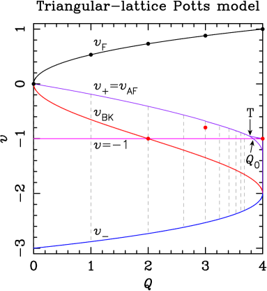
Figure 2: Phase diagram of the triangular-lattice $Q$-state Potts model in the real $(Q,v)$ plane. The cubic (12) corresponds to the three thick lines labeled $v_{\text{F}}$, $v_{\text{BK}}$, and $v_{-}$, respectively. The horizontal line corresponds to $v=-1$ (13). The curve between $v_{\text{F}}$ and $v_{\text{BK}}$ is our best numerical estimate of the AF curve $v_{+}=v_{\text{AF}}$ for this lattice [48]. This curve has a bifurcation point T, leading to two branches: one goes to the point $(Q_{0},-1)$ [cf. (19)], while the other goes to the critical point $(4,-1)$. The region defined by these three points and $(4,-1.253)$ is governed by the regime IV that we will consider hereafter, while the BK phase corresponds to regime I. (Compare to figure 1.) The vertical dashed lines correspond to the Beraha numbers $B_{k}$ [cf. (3)], shown here for $3\leq k\leq 11$. The solid dots depict the known critical points for integer values of $Q$.

A schematic phase diagram which is compatible with our current understanding is shown in figure 2. Let us parameterise the cubic curve (12) by

$$v\;=\;-1+2\cos\left(\frac{2\pi(1-g)}{3}\right)\,,\qquad Q\;=\;4\cos^{2}\left(\pi g\right)$$ (14)

where $-\frac{1}{2}\leq g\leq 1$. The range $0<g\leq 1$ then has then same CG interpretation as for the square lattice: $\frac{1}{2}\leq g\leq 1$ corresponds to $v_{\text{F}}$, and $0<g\leq\frac{1}{2}$ to $v_{\text{BK}}$. The interval $-\frac{1}{2}\leq g<0$ (corresponding to $v_{-}$) cannot be interpreted within this CG, but has been shown numerically [27] to belong to the same universality class [38, 39] as the antiferromagnetic curve (9) for the square-lattice Potts model (with the same value of $Q$).

This implies that the middle branch $v_{\text{BK}}$ of (12) will control the BK phase, which should extend from the lower branch of (12), that we hence identify with $v_{-}$, up to some AF transition curve $v_{\text{AF}}=v_{+}$, that unfortunately has not yet been determined analytically. This curve cannot be the chromatic line (13), since the latter is not always above the middle branch of (12). At the origin, $(Q,v)=(0,0)$, the AF curve describes a spanning-forest problem and its slope is known numerically [44]. It has be followed numerically to higher $Q$ in [48], and other pieces of yet unpublished work, and is depicted in figure 2.

Along the chromatic line $v=-1$, Baxter has found [17] three distinct analytic expressions for the TM eigenvalue $g_{i}$, whose logarithm is the bulk free energy (per site):

$$g_{1}(Q) = -\frac{1}{x}\prod_{j=1}^{\infty}\frac{(1-x^{6j-3})(1-x^{6j-2})^{2}(1-x^{6j-1})}{(1-x^{6j-5})(1-x^{6j-4})(1-x^{6j})(1-x^{6j+1})}\,,$$ (15)

$$\log g_{2}(Q) = \int_{-\infty}^{\infty}{\rm d}k\,\frac{\sinh k\theta}{2k}\left(\frac{\sinh[k(\pi-2\theta)/2]}{(2\cosh k\theta-1)\sinh(\pi k/2)}\right.$$ (16)

$$\qquad\qquad\qquad\qquad\left.-\frac{\cosh[k(\pi-2\theta)/2]}{(2\cosh k\theta+1)\cosh(\pi k/2)}\right)\,,$$

$$\log g_{3}(Q) = \int_{\infty}^{\infty}{\rm d}k\,\frac{\sinh k\theta\,[\sinh k(\pi-\theta)]}{k\sinh\pi k\,[2\cosh k(\pi-\theta)-1]}\,,$$ (17)

where we have parameterised

$$Q\;=\;2-x-x^{-1}\;=\;2+2\cos\theta\,,$$ (18)

with $|x|<1$ and $0<\text{Re}(\theta)<\pi$. (See Ref. [17] for details.)

In his second paper [18], Baxter determined the regions of $Q\in\mathbb{C}$ for which each of the expressions (15)–(17) is dominant (see figure 1). This was done by investigating the ratios $g_{2}/g_{1}$ and $g_{3}/g_{1}$, which can both the expressed as infinite products, by a combination of symmetry arguments and numerical analysis. His final result is:

1. $g_{1}$ is dominant for $Q\in(-\infty,0)\cup(4,\infty)$.

2. $g_{2}$ is dominant for $Q\in(Q_{0},4)$.

3. $g_{3}$ is dominant for $Q\in(0,Q_{0})$.

where [18, 10]

$$Q_{0}=3.819\,671\,731\,239\,719\cdots\,.$$ (19)

Returning now to the phase diagram in the $(Q,v)$-plane, the simplest scenario that can account for these findings is that the AF transition curve must split before $Q_{0}$ into a branch that goes down to $(Q,v)=(Q_{0},-1)$ and delimits the BK phase, and another branch that extends further to the 4-colouring point $(Q,v)=(4,-1)$. This scenario, which is shown schematically in figure 2, is confirmed by studies of the limiting curves and the critical polynomial [48]. The region $v<-1$ appears to contain further intricate features, which are beyond the scope of the present discussion.

The region (i) where $g_{1}$ dominates is non-critical. In that region, exact expressions for the surface and corner free energies are also known [29], and the contributions from corners of angle $\frac{\pi}{3}$ and $\frac{2\pi}{3}$ can even be determined separately [30]. In the limit $Q\to 4^{+}$, these corner free energies develop essential singularities that have been determined from the asymptotic analysis of the exact expressions [30].

For the remainder of this paper we shall restrict the attention to the critical regions (ii) and (iii). For reasons that will become clear from the mappings in section 3 to a spin-one vertex model, we shall refer to the critical theory that dominates in region (iii) as regime I, and to the theory dominating (ii) as regime IV. (See figure 1.) Our objective is to extend Baxter’s analysis to compute the exact critical exponents in either of these regimes, and determine the corresponding CFT.

Regime I is relatively straightforward to deal with, using the mapping to the O($n$) model [19] and the BA analysis of the associated 7-vertex model [21]. Choosing a particular twist of the vertex model to ensure the equivalence with the Potts model will enable us to compute the corresponding critical exponents; see section 4.2. The end result is that regime I is also described by the BK universality class. It is remarkable that the triangular-lattice Potts model has two distinct integrable curves, (13) and the middle branch of (12), with the same critical behaviour.

Regime IV is our main interest here. It cannot be obtained within the 7-vertex model [21], and indeed in that reference the existence of the region $Q\in(Q_{0},4)$ was relegated to a terse footnote. However, using further mappings to a 19-vertex model (see section 3), we shall obtain an efficient handle on regime IV and derive the corresponding critical exponents and CFT interpretation. Achieving this is going to be the principal motivation for the remainder of this paper.

Remarks. 1. Although Baxter’s analysis of the eigenvalues (15)–(17) has been subject of some debate [10]—in particular concerning the precise numerical evaluation of the infinite products—his conclusions for $Q\in\mathbb{R}$ have withstood a number of stringent numerical tests [48].

2. In the square-lattice case, we could say that $Q_{0}=3$. The corresponding chromatic polynomial does not define an integrable theory. However, since the region $0\leq Q<Q_{0}$ is attracted to $v_{\rm BK}$ under the renormalisation group flow, it can be identified with regime I. The behaviour right at $Q=Q_{0}$ is given instead by the AF curve $v_{+}$.

3. The extension of Baxter’s work to the computation of critical exponents, by means of a BA analysis, is deferred to section 4, where a twist should be included in the BA equations.

3 From the chromatic polynomial to a spin-one vertex model

Baxter [17] found an ingenious coordinate BA for the triangular-lattice chromatic polynomial, involving several kinds of particle trajectories (that he represented as dotted, full, double-full and wiggly lines). In view of the subsequent developments in the classification of integrable systems, it appears preferable to instead bring the chromatic polynomial into contact with a (by now) well-studied integrable model to which we can apply all the (by now) standard BA machinery. In this section we therefore reexpress the colouring problem in terms of an integrable, spin-one vertex model on the square lattice, known as the Izergin–Korepin (IK) (or $a_{2}^{(2)}$) model.

The route that we shall take passes through quite a number of different formulations as intermediate steps. We emphasise that although each of the mappings exhibited here is exact, the various models appearing have different domains of validity. Some require $Q\in\mathbb{N}$, while other allow for any $Q\in\mathbb{R}$; sometimes the twist (that determines the weight of non-contractible clusters and loops) is a free parameter, and sometimes it is fixed. In more technical terms, each model provides a distinct representation of the underlying Temperley-Lieb (or dilute TL) algebra, which is not always faithful with respect to the most general formulation (allowing for arbitrary values of $Q$ and the twist). It follows that some of the eigenstates—and hence some of the critical exponents—are absent from some of the models presented, and not all of the correlation functions can be directly interpreted in terms of the original colouring problem. To keep track of these subtleties, our discussion puts a special emphasis on the definition of the corresponding transfer matrices, as well as on the various physical observables of interest.

Another key point is to keep carefully track of the twist. The bulk free energy obtained by Baxter [17] is independent on the twist, so he did not need to introduce it. However, since we are eventually aiming at exact expressions for the critical exponents—which are sensitive to the boundary condition defined by the twist—we need to ensure that each model in the series of mappings is identically twisted.

It is worth stressing that we will start from the colouring problem defined on a strip of the triangular lattice with cylindrical boundary conditions and a width $L$ multiple of 3. This choice allows for a 3-colouring for such strips, with vertices of each of the three sublattices having constant colour. Strip graphs of widths $L$ not a multiple of 3 correspond to a topologically frustrated ground state, depending on the value of $L\pmod{3}$, and will be considered elsewhere [50].

3.1 Colouring problem

We start from the Potts model defined on a strip of the triangular lattice $G=(V,E)$, whose partition function we recall to be given by

$$Z^{\rm Potts}_{G}(Q,K)\;=\;\sum_{\{\sigma_{i}\}}\,\prod_{\langle i,j\rangle}\,\mathrm{e}^{K\,\delta_{\sigma_{i},\sigma_{j}}}\,,$$ (20)

where $Q\in{\mathbb{N}}$ and $K\in{\mathbb{R}}$. The colouring problem is recovered for $K\to-\infty$. Viewing the longitudinal direction of the strip as imaginary time, we can build the system row by row acting with the TM, which we represent as follows:

where the dashed lines indicate that the two ends are to be joined to recover the cylinder geometry.

For generic values of $K$, the TM in this spin representation acts on the space of all spin configurations of a given row, $\{1,2,\ldots,Q\}^{L}$. Therefore, its dimension is given simply by $Q^{L}$. In the colouring problem ($K=-\infty$) this dimension is reduced because of the nearest-neighbour constraint $\sigma_{i}\neq\sigma_{j}$. In terms of the corresponding colouring matrix $A=\{1-\delta_{\sigma_{i},\sigma_{j}}\}_{1\leq i,j\leq Q}$ the dimension reads $d_{L}={\rm Tr}\ A^{L}$. Now $A$ has one eigenvector $v_{1}(\sigma_{i})=1$ with eigenvalue $Q-1$, and $Q-1$ eigenvectors $v_{k}(\sigma_{i})=\delta_{\sigma_{i},1}-\delta_{\sigma_{i},k}$, for $k=2,3,\ldots,Q$, each with eigenvalue $-1$. Therefore $d_{L}=(Q-1)^{L}+(Q-1)(-1)^{L}$, which obviously grows asymptotically as $(Q-1)^{L}$. Note that $d_{L}$ can be further reduced by taking into account the (transverse) translational symmetry of the strip.

The main drawback of the TM method in the spin representation is that for each value of $Q\in\mathbb{N}$ we have to produce a distinct TM.

We now turn to the physical correlation functions and critical exponents of interest in the colouring problem. The first of these is the so-called magnetic correlation function, defined between two sites $i,j$ of the triangular lattice as

$$G_{H}(i,j)\;=\;\left\langle\delta_{\sigma_{i},\sigma_{j}}-\frac{1}{Q}\right\rangle\,.$$ (21)

On the critical lines of the phase diagram, the magnetic correlation function has an algebraic asymptotic behaviour:

$$G_{H}(i,j)\;\sim\;|i-j|^{-2x_{H}}\,,\qquad\text{for $|i-j|\gg 1$}\,,$$ (22)

where $x_{H}$ is the magnetic exponent. Away from critical points, it decays exponentially fast with the distance, $G_{H}(i,j)\sim\rm{e}^{-|i-j|/\xi}$, with a typical length scale given by the correlation length $\xi$. The asymptotic behaviour of the correlation length in the vicinity of a critical point allows for the definition of another critical exponent:

$$\xi(v)\;\sim\;|v-v_{c}|^{-\nu}\,,$$ (23)

which is related to the thermal exponent $x_{T}$ through

$$\nu\;=\;\frac{1}{2-x_{T}}\,.$$ (24)

Two-point functions of more general operators, acting on groups of more than one spin, have been defined in [51]. They include in particular the so-called $k$-cluster ‘watermelon’ operators, which can however be formulated more easily in the FK representation to which we turn next.

3.2 FK representation

The partition function (20) can be rewritten in the FK representation as follows [22]:

$$Z^{\rm FK}_{G}(Q,v)\;=\;\sum_{A\subseteq E}v^{|A|}\,Q^{k(A)}\,,$$ (25)

where $v=\mathrm{e}^{K}-1=-1$ in the colouring problem, and $k(A)$ is the number of connected components of the spanning subgraph $(V,A)$. As this function is a polynomial in both $Q$ and $v$, we can extend those variables analytically to arbitrary real or even complex numbers. The original colouring model is in principle recovered when we specialise (25) to $v=-1$ and $Q\in{\mathbb{N}}$; however one must ensure that the free energy and the correlation functions obtained in the cluster representation still make sense in the colouring problem. Whether this is true or not depends, as we will see, on the regime under consideration.

As in the spin representation, we can define the FK representation of the TM on the triangular lattice, with the important difference that the latter considers all values of $Q\in{\mathbb{C}}$ at the same time. The computation of the TM for a triangular-lattice strip with cylindrical boundary conditions is not straightforward: one needs to consider first a strip of width $L+1$ with free transverse boundary conditions, and at the end, identify sites $1$ and $L+1$ [18, 8]. The final TM acts on the space of all non-crossing, non-nearest-neighbour partitions of the set $\{1,2,\ldots,L\}$ on a circle. The non-crossing property is due to the planarity of the graph, and the non-nearest-neighbor property is due to $v=-1$ (i.e., neighbour spins cannot be coloured alike) [8, 29]. The number of such partitions is given by the Riordan number $R_{L}$ for $L\geq 2$; its asymptotic behaviour is $R_{L}=3^{L}L^{-3/2}3\sqrt{3}/(8\sqrt{\pi})[1+O(1/L)]$ (see e.g. ref. [8, section 3.3 and references therein]). If we also take into account the translational symmetry along the transverse direction, the number of partition classes modulo translations is asymptotically equal to $R_{L}/L$.

Turning to physical observables, the magnetic correlation function (21) gets straightforwardly translated in the FK representation as

$$G_{H}(i,j)\;=\;\frac{Q}{Q-1}\,\frac{Z_{G}^{(i\leftrightarrow j)}(Q,v)}{Z_{G}^{\text{FK}}(Q,v)}\,,$$ (26)

where $Z_{G}^{(i\leftrightarrow j)}$ is the partition sum of FK configurations where sites $i$ and $j$ belong to the same cluster. In the TM picture, the points $i$ and $j$ get mapped onto the infinite top and infinite bottom of the cylinder, and the exponent $x_{H}$ can be obtained from the scaling of the TM eigenvalues as

$$\log\left|\frac{\Lambda_{0}^{(L)}}{\Lambda_{1}^{(L)}}\right|\;=\;\frac{2\pi G\,x_{H}}{L}+o\left(\frac{1}{L}\right)\,,$$ (27)

where $G=\frac{\sqrt{3}}{2}$ is a geometrical factor [10], $\Lambda_{0}^{(L)}$ is the largest TM eigenvalue, and $\Lambda_{1}^{(L)}$ is the largest eigenvalue in the subsector where one cluster (considered ‘marked’) is imposed to propagate along the vertical direction of the cylinder, and hence cannot be destroyed by the action of the TM. This definition can actually be extended, as we can enlarge our state space by imposing the propagation of $k$ distinct marked clusters from the bottom to the top of the cylinder, leading to the set of exponents

$$\log\left|\frac{\Lambda_{0}^{(L)}}{\Lambda_{k}^{(L)}}\right|\;=\;\frac{2\pi G\,x_{k}}{L}+o\left(\frac{1}{L}\right)\,.$$ (28)

The case $k=1$ actually contains two distinct situations, depending whether the propagating cluster is allowed to wrap around the cylinder or not; we will come back to this issue in section 3.4.

In a similar fashion, we expect that the thermal exponent should be related to the relative scaling of the subdominant eigenvalue $\Lambda_{0}^{\prime(L)}$ in the $k=0$ sector, with respect to the dominant one $\Lambda_{0}^{(L)}$, namely

$$\log\left|\frac{\Lambda_{0}^{(L)}}{\Lambda_{0}^{\prime(L)}}\right|\;=\;\frac{2\pi G\,x_{T}}{L}+o\left(\frac{1}{L}\right)\,.$$ (29)

Remark. It is worth mentioning that for $Q=B_{p}$ [cf. (3)], with integer $p\geq 3$, the Potts-model partition function allows for another probabilistic interpretation (with positive weights), namely in terms of a restricted-solid-on-solid (RSOS) model [37, 52]. We will discuss this issue in section 6.

3.3 Duality transformation

Given a $Q$-state Potts model with parameter $v$ in the FK representation (25) and defined on a triangular lattice $G=(V,E)$, a duality transformation [53] allows us to obtain an equivalent $Q$-state Potts model on the dual, hexagonal lattice $G^{*}=(V^{*},E^{*})$, by putting a FK link on each edge of $E^{*}$ not crossed by a FK link on $E$ (see figure 3).

Figure 3: Configuration of FK clusters on the triangular lattice $G$ (black), and the associated configuration of dual FK clusters on the hexagonal lattice $G^{*}$ (blue). In red, we have represented the surrounding loops on the medial, kagome lattice.

The corresponding dual parameter is given by

$$v^{*}\;=\;\frac{Q}{v}\;=\;-Q\,,$$ (30)

and we can represent the corresponding TM as

where the dual, hexagonal lattice has been represented in blue. The space of states in terms of a set of connectivities follows from a construction analogous to that used on the triangular lattice, and we point out that imposing a number $k$ of propagating clusters in the triangular-lattice Potts model is equivalent to imposing the same number of propagating clusters in the dual, hexagonal-lattice model, so that the definition of critical exponents sketched in the previous section translates straightforwardly to the dual model.

Note that under duality the chromatic polynomial $\chi_{G}$ of a planar graph $G$ transforms into the flow polynomial $\Phi_{G^{*}}$ on the dual graph $G^{*}$. To be more precise, $\chi_{G^{*}}(Q)=Q\,\Phi_{G}(Q)$.

3.4 Six-vertex model on the kagome lattice

The Potts model on the dual, hexagonal lattice $G^{*}$, can be further mapped mapped onto a model of loops living on the edges on the medial, kagome lattice, and corresponding to the surrounding contours of the FK clusters in the spanning subgraph $(V^{*},A)$ (see figure 3). This is achieved through the following identity [54]

$$Z^{\rm FK}_{G^{*}}(Q,v^{*})\;=\;Q^{|V^{*}|/2}\,\sum\limits_{A\subseteq E^{*}}(x^{*})^{|A|}\,Q^{\ell(A)/2}\,,$$ (31)

where $\ell(A)$ counts the number of loops in the spanning subgraph $(V^{*},A)$, and

$$x^{*}\;=\;\frac{v^{*}}{\sqrt{Q}}=-\sqrt{Q}\,.$$ (32)

The configurations of this loop model can now be mapped onto those of a six-vertex model on the kagome lattice [49]. This is done by reexpressing the factor $Q^{\ell(A)/2}$ in terms of local factors by setting [cf. (18)]:

$$\sqrt{Q}\;=\;2\cos\frac{\theta}{2}\,,$$ (33)

and summing over the orientations of loops, as represented in the first two lines of figure 4. Notice that in this figure we represent only one of the possible three types of vertices on the kagome lattice (related by $2\pi/3$ rotations); however, contrary to what happens for the square lattice, we can always see which weights are which because the two angles in the kagome lattice are distinct: $\pi/3$ and $2\pi/3$, respectively.

The TM of the resulting six-vertex model can be represented as follows (the vertices and edges of the medial kagome lattice are depicted as red dots and lines, respectively):

The degrees of freedom are now the orientations on each edge of the kagome lattice, so the TM acts on each row on the space of $2L$ edges oriented either upwards and downwards, therefore with a total dimension $2^{2L}=4^{L}$.

As suggested by the figure above, a twist factor $\mathrm{e}^{\pm i\frac{\varphi}{2}}$ has to be introduced in the six-vertex model in order to ensure the correspondence with the original periodic Potts model. It is represented by a red wavy line, which contributes a factor $\mathrm{e}^{\pm i\frac{\varphi}{2}}$ each time it is crossed by a rightwards (resp. leftwards) arrow of the six-vertex model. The twist parameter ${\varphi}$ must be chosen as follows:

• In the sector with no propagating clusters ($k=0$), there may be closed loops on the kagome lattice, that wind around the transverse periodic boundary condition. To recover the original model, these loops must be given the same weight $\sqrt{Q}=2\cos\frac{\theta}{2}$ as the one given to contractible loops. Choosing the twist $\frac{\varphi}{2}=\frac{\theta}{2}$ (or, as we shall see, $\frac{\varphi}{2}=\frac{2\pi-\theta}{2}$, depending on the regime), since each loop has to be summed over the two possible orientations, it is given a weight

  $$\mathrm{e}^{i\frac{\varphi}{2}}+\mathrm{e}^{-i\frac{\varphi}{2}}\;=\;2\cos\frac{\theta}{2}\,,$$ (34)

  as required. Therefore we expect the central charge of the Potts model to be given in terms of the free energy (density per site) by [55, 56]

  $$f_{L}(\varphi)\;=\;\frac{1}{L}\,\log\left|{\Lambda_{0}^{(L)}}(\varphi)\right|\;=\;f_{\text{bulk}}+\frac{\pi G\,c}{6L^{2}}+o\left(\frac{1}{L^{2}}\right)\,,$$ (35)

  where $\Lambda_{0}^{(L)}(\varphi)$ is the largest eigenvalue of the six-vertex TM, appropriately twisted, in the sector with $\ell=0$ ‘through-lines’ (Potts loops propagating along the vertical direction of the cylinder).

• In the sector with a single propagating FK cluster ($k=1$) we have two distinct situations:

  • If the propagating FK cluster is allowed to wrap around the cylinder, then this translates in the six-vertex language to no loop propagating in the vertical direction, but no closed loop allowed to wrap around the cylinder. Forbidding loops on the kagome lattice to wrap around the cylinder amounts to giving such loops a weight $0$, therefore to fixing the twist to $\frac{\varphi}{2}=\frac{\pi}{2}$. The magnetic exponent can thus be obtained as

    $$\log\left|\frac{\Lambda_{0}^{(L)}(\varphi)}{\Lambda_{0}^{(L)}(\pi)}\right|\;=\;\frac{2\pi G\,x_{H}}{L}+o\left(\frac{1}{L}\right)\,.$$ (36)

  • If the propagating FK cluster is not allowed to wrap around the cylinder, then it translates in the Potts loops/six-vertex language into the presence of two loops propagating in the vertical direction (‘through-lines’) delimiting the vertical borders of the propagating FK cluster. The situation is then similar to the case $k\geq 2$, described in the following paragraph.

• In the sectors with $k\geq 2$ propagating clusters (or $k=1$ cluster not allowed to wrap around the cylinder, see above), there are no non-contractible loops anymore. Each propagating cluster is associated with two Potts through-lines, and one can take each of the $\ell=2k$ through-lines around the axis of the cylinder without affecting the Boltzmann weights, if every such line acquires in doing so a phase which is a $\ell^{\rm th}$ root of unity. This means that the eigenvalues of the original model are obtained in the twisted vertex model with a twist being of the form $\frac{2\pi p}{\ell}$, with any integer $p$ satisfying $\gcd(p,\ell)=1$.

Figure 4: Mapping from the Potts model (31) on the hexagonal lattice (first line) onto a six-vertex model on the kagome lattice (second line), and then onto a model of dilute loops on the hexagonal lattice (third line).

3.5 O$(n)$ model on the hexagonal lattice

As shown in the last line of figure 4, the configurations of the six-vertex model can in turn be mapped onto those of dilute loops living on the edges on the hexagonal lattice. In this mapping, the thin spin-$\frac{1}{2}$ loops run around the inside and outside of the thick spin-$1$ loops, therefore a dilute loop on the hexagonal lattice is a double Potts loop on the kagome lattice.

The resulting gas of dilute loops is nothing but the O$(n)$ model on the hexagonal lattice [19], where the weight of each closed loop is

$$n\;=\;-2\cos 2\theta$$ (37)

and the fugacity of each loop segment is

$$K\;=\;\frac{1}{2\sin\frac{\theta}{2}}$$ (38)

The corresponding TM can be represented as follows:

One needs to be careful about what becomes in this model of the twist parameter introduced in the six-vertex model: each loop segment of the O$(n)$ model crossing the vertical seam has to be summed over two possible orientations. Now, from figure 4, one sees that each oriented O$(n)$ loop crossing the vertical seam is equivalent to two edges of the six-vertex model crossing the seam with the same orientation, hence a twist $\varphi$ rather than $\frac{\varphi}{2}$ (where $\varphi$ has to be conveniently chosen depending on the sector we are considering, as explained in the previous section).

It is important to stress that making the right choice for the twist in order to ensure the correspondence with the original periodic Potts model results in a ‘wrong’ choice of the weight for non-contractible loops in the O$(n)$ model. For instance, in the $k=0$ sector, if we choose $\frac{\varphi}{2}=\frac{\theta}{2}$, we get the right weight for the winding FK clusters $\sqrt{Q}=2\cos\frac{\theta}{2}$; but the wrong one for the winding O($n$) loops $\widetilde{n}=2\cos\theta$. Similarly, if we choose $\frac{\varphi}{2}=\theta-\frac{\pi}{2}$, we get the right weight for a winding O($n$) loop $n=-2\cos 2\theta$, but the wrong one for a winding FK cluster $\widetilde{Q}^{1/2}=2\sin\theta$. In other words, the periodic Potts model is equivalent to a O$(n)$ model on the hexagonal lattice with a particular choice of twisted boundary conditions.

The TM acts on the set of non-crossing dilute matchings of the set $\{1,2,\ldots,L\}$. By dilute (in opposition to perfect) we here mean that any given point may be empty and hence not paired with another point. The number of such matchings is given by the Motzkin number $M_{L}$ for $L\geq 1$; its asymptotic behaviour is $3^{L}L^{-3/2}3\sqrt{3}/(2\sqrt{\pi})[1+O(1/L)]$.

3.6 Spin-one vertex model on the square lattice

The O$(n)$ model on the hexagonal lattice is a particular case of the O$(n)$ model on the square lattice, whose vertex weights are parameterised as shown in the first line of figure 5.

Figure 5: Vertices of the square lattice O$(n)$ loop model (first row), together with the corresponding Boltzmann weights, and their mapping onto the vertices of the hexagonal lattice O$(n)$ model when the weight $\rho_{9}$ is zero.

Indeed, in the particular case $\rho_{9}=0$, the vertices can be stretched horizontally by adding one additional horizontal edge as shown in the second line of the figure.

An integrable choice of the Boltzmann weights is well known [57] (we use here the notations of [58]):

$$\rho_{1}(u) \;=\;1+\frac{2\cos(u+\frac{3\theta}{2})\sin u\sin\frac{\theta}{2}}{(2\cos\theta-1)\sin^{2}\theta}\,,$$ (39a)

$$\rho_{2}(u) \;=\;\rho_{3}(u)\;=\;\frac{\cos(u+\frac{3\theta}{2})}{\cos\frac{3\theta}{2}}\,,$$ (39b)

$$\rho_{4}(u) \;=\;\rho_{5}(u)\;=\;-\frac{\sin u}{\cos\frac{3\theta}{2}}\,,$$ (39c)

$$\rho_{6}(u) \;=\;\rho_{7}(u)\;=\;\frac{2\cos(u+\frac{3\theta}{2})\sin u\sin\frac{\theta}{2}}{(2\cos\theta-1)\sin^{2}\theta}\,,$$ (39d)

$$\rho_{8}(u) \;=\;\frac{\sin(2u+\frac{5\theta}{2})-\sin\frac{\theta}{2}}{2(\cos\theta+\cos 2\theta)}\,,$$ (39e)

$$\rho_{9}(u) \;=\;\frac{\cos(u+\frac{\theta}{2})\sin u}{2\cos^{2}\frac{\theta}{2}\sin\frac{\theta}{2}(2\cos\theta-1)}\,.$$ (39f)

In all the following we rescale $\rho_{4}$ and $\rho_{5}$ by a factor $-1$, which is just a change of basis. This model has several symmetries:

• The transformation $u\to\frac{3\pi}{2}-\frac{3\theta}{2}-u$ for fixed $\theta$ is equivalent to rotating the vertices of figure 5 through $\frac{\pi}{2}$ (crossing symmetry).

• Up to some gauge symmetry, the weights are also invariant under $\pi$ shifts of $u$, as well as under $2\pi$ shifts of $\theta$.

For a given $\theta$, there is only one non-trivial value of the spectral parameter $u$ such that $\rho_{9}=0$, namely $u=\frac{\pi}{2}-\frac{\theta}{2}$. The corresponding weights, which we rescale such that $\rho_{1}=1$, are the following [cf. (39)]:

$$\rho_{1} \;=\;1\,,$$ (40a)

$$\rho_{2} \;=\;\rho_{3}\;=\;\frac{1}{2\sin\frac{\theta}{2}}\,,$$ (40b)

$$\rho_{4} \;=\;\ldots\;=\;\rho_{8}\;=\;\frac{1}{4\sin^{2}\frac{\theta}{2}}\,,$$ (40c)

$$\rho_{9} \;=\;0\,,$$ (40d)

so they recover precisely the fugacity $K$ given by eq. (38).

Now, it is well-known (see [58] for a review) that the integrable O$(n)$ model on the square lattice can be reformulated as a spin-one vertex model, the so-called IK (or $a_{2}^{(2)}$) model. The equivalence is worked out by once again giving orientations to the loops (to be summed over), and turning the loop weight $n$ into local, angular contributions. Each occupied edge is associated with a state $\pm 1$ (depending on the orientation of the corresponding loop), while empty edges are associated with the state $0$.

We can now bend the lattice, and represent the corresponding TM as follows:

where each edge carries a $S^{(z)}=-1,0,1$ state, the interactions are encoded by local vertex weights depending on the 19 possible states of the adjacent edges, and the vertical seam (red wavy line) corresponds to a boundary twist $\mathrm{e}^{-i\varphi},1,\mathrm{e}^{i\varphi}$. The fact that the vertical seam now only crosses one horizontal edge of each row (whereas it also crosses the last “vertical” edge in the six-vertex formulation on the kagome lattice) is irrelevant, since the vertical crossing can be eliminated by a change of basis.

The TM of the model commutes with the total magnetization

$$m\;=\;\sum_{i=1}^{L}S^{(z)}_{i}\,,$$ (41)

which can naturally be associated to the number of through-lines in the O$(n)$ loop formulation. Therefore each sector of fixed $m$ can be considered independently.

Rather than checking now explicitly that the eigenvalues dominating the spectrum of the TM for the different sectors of the colouring problem are indeed recovered by the spin-one vertex model, we defer this discussion to the next section, where we will deal with the BA construction of these different eigenvalues.

The total dimension of the spin-one vertex model TM, summed over all magnetisation sectors $m$, is obviously $3^{L}$. In the $m=0$ sector the dimension is given by the central trinomial coefficient, that is, the largest coefficient in the expansion of $(1+x+x^{2})^{L}$. This has asymptotic behaviour $3^{L}L^{-1/2}\sqrt{3/4\pi}[1+O(1/L)]$. Similarly, the dimension in sector $m=1$ is given by the next-to-central trinomial coefficient, and more generally, that of the sector with magnetisation $m$ by the trinomial coefficient that is $m$ places away from the centre.

We stress that these dimensions are larger than those of the O$(n)$ loop model, for the reason that the TM of the latter does not distinguish between contractible and non-contractible loops (it gives a weight $n$ to either type of loop). It is however possible to work with an ‘augmented’ loop model TM in which each arc connecting two points is distinguished by the parity (even or odd) of the number of times it has crossed the vertical seam. When closing an even (resp. odd) arc we obtain a contractible (resp. non-contractible) loop. It is easy to see that states of this augmented loop model are in bijection with those of the spin-one vertex model. It follows by the above equivalences that the spectra of the respective TM are identical.

4 Bethe Ansatz solution

After all the mappings of section 3, we have managed to reformulate the original colouring problem as an integrable spin-one model, namely the $a_{2}^{(2)}$ model with a particular value of the twist, related to the weight of non-contractible FK clusters. This means that we are now in a good position to apply the toolbox of the BA method.

The goal of the present section is to set up the general framework, and define properly the regimes I and IV that were introduced in section 2.4, as well as the possible excitations of the ground state configuration at finite size $L$. With these ingredients at hand, we can then in section 5 take the continuum limit and work out the corresponding critical exponents.

4.1 Bethe Ansatz equations

It is well-known how to construct the eigenstates of the integrable spin-one model through the BA. Each eigenstate is parameterised by a set of Bethe roots, solution of the Bethe Ansatz equations (BAE). In our particular case, the BAE for the square-lattice O($n$) model (which is related to the IK model) are given by:

$$\left(\frac{\sinh\left(\lambda_{j}-\mathrm{i}\frac{\theta}{2}\right)}{\sinh\left(\lambda_{j}+\mathrm{i}\frac{\theta}{2}\right)}\right)^{L}\;=\;\mathrm{e}^{\mathrm{i}\varphi}\;\prod\limits_{i(\neq j)}\frac{\sinh\left(\lambda_{j}-\lambda_{i}-\mathrm{i}\theta\right)\cosh\left(\lambda_{j}-\lambda_{i}+\mathrm{i}\frac{\theta}{2}\right)}{\sinh\left(\lambda_{j}-\lambda_{i}+\mathrm{i}\theta\right)\cosh\left(\lambda_{j}-\lambda_{i}-\mathrm{i}\frac{\theta}{2}\right)}\,.$$ (42)

From there, we look for the leading TM eigenstates of the colouring problem in terms of Bethe roots for an appropriate twist. The following conclusions have been known since the paper of Baxter [18]:

• The range $0<Q<Q_{0}$ is described by the so-called regime I in the notations of [59]. Namely the ground state is made of roots with imaginary part $\frac{\pi}{2}$.

• The $Q_{0}<Q<4$ regime is dominated by another configuration of roots [17], namely $\frac{2L}{3}$ real roots, and $\frac{L}{3}$ roots with imaginary part $\frac{\pi}{2}$. It is worth noting that the corresponding eigenstates are absent from the loop formulations, both on the square and hexagonal lattice. Also, it never dominates at one of the isotropic values of the spectral parameter studied in [59, 58], nor does it dominate the spectrum of the corresponding Hamiltonians, obtained by differentiating the TM with respect to the spectral parameter $u$, at the value $u=0$. As a consequence, this regime has escaped the attention of previous works on the IK vertex model, in which three regimes labelled I, II and III were identified and studied [59, 58]. Extending this nomenclature, we shall call the regime dominated by this root configuration regime IV.

Before going further in the study of the regimes, let us compare the BAE (42) with those of [17, 21], where a 7-vertex formulation of the hexagonal-lattice O$(n)$ loop model is solved without any reference to the IK 19-vertex model, which, as we have seen, is related to the more general square-lattice O($n$) loop model. The BAE are written in terms of a set of complex Bethe roots $\{z_{j}\}$, and read

$$z_{j}^{L}\;=\;(-1)^{n-1}\,\mathrm{e}^{i\epsilon}\,\prod_{i(\neq j)}\frac{S(z_{i},z_{j})}{S(z_{j},z_{i})}\,,$$ (43)

where the scattering phases are

$$S(z,w)\;=\;\left(1-z-w+zw+t^{2}z\right)\left(1-2w+zw+t^{2}w\right)\,,$$ (44)

and $t^{2}=2-2\cos\theta$. In (43), we use the parameter $n=L+n_{-}-n_{+}$ equal to the number of lines in Baxter’s formulation [17], with $n_{+}$ (resp. $n_{-}$) being the number of upward (resp. downward) pointing vertical arrows in each row [21]. Our sector $k=0$ corresponds to $n_{-}=n_{+}$, hence $n=L$. Following [21], we set $z_{j}=\frac{1+rw_{j}}{r+w_{j}}$, where $r=\mathrm{e}^{i\theta}$; however, while these authors [21] further define $w_{j}=\mathrm{e}^{2\lambda_{j}}$, we choose instead to set $w_{j}=-\mathrm{e}^{2\lambda_{j}}$. From there, the BAE (43) are easily seen to take the form (42), where the correspondence between the twist parameters is simply $\varphi=\epsilon$. In other words, the BAE underlying the construction of eigenstates for the two models (the 7-vertex model of [21] and the IK 19-vertex model) are the same, even though the space of states of the two models are not equivalent.

4.2 Regime I: Summary of its properties

Regime I, originally investigated in the context of the square lattice [59], was studied in great detail for the O($n$) loop model on the hexagonal lattice in [21]. The CFT is that of a single compactified bosonic field, and in particular, the dependence of the central charge $c$ on the twist $\varphi$ was exactly found to be

$$c(\varphi)\;=\;1-\frac{3\varphi^{2}}{\pi\theta}\,,$$ (45)

while the set of exponents with respect to the untwisted central charge $c=1$ were found as

$$\Delta_{m,w}\;=\;\frac{m^{2}\theta}{4\pi}+w^{2}\frac{\pi}{\theta}\,,$$ (46)

and therefore, with respect to the twisted theory (45),

$$x_{m,w}\;=\;\frac{m^{2}\theta}{4\pi}+w^{2}\frac{\pi}{\theta}-\frac{\varphi^{2}}{4\pi\theta}\,,$$ (47)

where $m$ the total magnetization introduced in (41), and $w$ can be thought of as related to the electric charge in the CG picture.

It turns out that the ground state of the O$(n)$ model with twist $\varphi=\theta$ is not observed in the Potts-model spectrum, and the central charge of the Potts model is recovered by choosing the twist in this regime as $\varphi=2\pi-\theta$. Then (45) reduces to

$$c_{\text{Potts}}\;=\;1-\frac{3(2\pi-\theta)^{2}}{\pi\theta}\;=\;1-\frac{6(p-1)^{2}}{p}\,,$$ (48)

where we have parameterised $\theta=2\pi/p$. This is precisely the central charge for the BK phase found by Saleur [47, 32], matching the CG results for coupling $g=\frac{1}{p}\in(0,\frac{1}{2})$. The $\ell$-leg watermelon exponents are straightforwardly obtained from (47), namely

$$x_{\frac{\ell}{2},0}\;=\;\frac{\ell^{2}\theta}{16\pi}-\frac{(2\pi-\theta)^{2}}{4\pi\theta}\;=\;\frac{\ell^{2}}{8p}-\frac{(p-1)^{2}}{2p}\,,$$ (49)

and coincide with the known values for bulk watermelon exponents in the BK phase (see for instance [60, 61]). As explained in section 3.4, the magnetic exponent is associated to the scaling of the TM eigenvalue with twist $\frac{\varphi}{2}=\frac{\pi}{2}$, namely

$$x_{H}\;=\;\frac{1}{12}\left(c_{\text{Potts}}-c(\pi)\right)\;=\;\frac{p}{8}-\frac{(p-1)^{2}}{2p}\,,$$ (50)

which once again coincides with the known value in the BK phase. The thermal exponent is obtained from the scaling of the subdominant eigenvalues in the ground state ($m=0,w=0$) sector. These are obtained by taking values of the twist parameter shifted by $2\pi$, namely $\varphi=2\pi(1+j)-\theta$, resulting in

$$x_{T}^{(j)}\;=\;\frac{1}{12}\left(c_{\text{Potts}}-c(2\pi(1+j)-\theta)\right)\;=\;\frac{j}{2}\left[(j+2)p-2\right]\,.$$ (51)

The two most relevant of these exponents (excluding the case $j=-1$, not observed in the spectrum) correspond to $j=1$ and $j=-2$, hence respectively

$$x_{T}\;=\;x_{T}^{(1)}\;=\;\frac{3p}{2}-1\;\geq\;2\,,\qquad x_{T}^{\prime}\;=\;x_{T}^{(-2)}\;=\;2\,.$$ (52)

Recalling that $p=\frac{1}{g}$, the first of these coincides with eq. (11).

4.3 Regime IV: structure of the leading eigenlevels

We now study in detail the so-called regime IV. Let us set notations: For sizes $L\in 3\mathbb{N}$, the ground state is described by $m_{1}=\frac{2L}{3}$ real roots $x_{i}$, and $m_{2}=\frac{L}{3}$ roots with imaginary part $\frac{\pi}{2}$ that we denote $y_{k}+\mathrm{i}\frac{\pi}{2}$ with $y_{k}\in\mathbb{R}$.

The Bethe equations (42) can be recast as:

$$\left(\frac{\sinh\left(x_{j}-\mathrm{i}\frac{\theta}{2}\right)}{\sinh\left(x_{j}+\mathrm{i}\frac{\theta}{2}\right)}\right)^{L} = \mathrm{e}^{\mathrm{i}\varphi}\,\prod_{i(\neq j)}\frac{\sinh\left(x_{j}-x_{i}-\mathrm{i}\theta\right)\cosh\left(x_{j}-x_{i}+\mathrm{i}\frac{\theta}{2}\right)}{\sinh\left(x_{j}-x_{i}+\mathrm{i}\theta\right)\cosh\left(x_{j}-x_{i}-\mathrm{i}\frac{\theta}{2}\right)}$$ (53)

$$\quad\times\,\prod_{k}\frac{\cosh\left(x_{j}-y_{k}-\mathrm{i}\theta\right)\sinh\left(x_{j}-y_{k}+\mathrm{i}\frac{\theta}{2}\right)}{\cosh\left(x_{j}-y_{k}+\mathrm{i}\theta\right)\sinh\left(x_{j}-y_{k}-\mathrm{i}\frac{\theta}{2}\right)}\,,$$

$$\left(\frac{\cosh\left(y_{k}-\mathrm{i}\frac{\theta}{2}\right)}{\cosh\left(y_{k}+\mathrm{i}\frac{\theta}{2}\right)}\right)^{L} = \mathrm{e}^{\mathrm{i}\varphi}\,\prod_{l(\neq k)}\frac{\sinh\left(y_{k}-y_{l}-\mathrm{i}\theta\right)\cosh\left(y_{k}-y_{l}+\mathrm{i}\frac{\theta}{2}\right)}{\sinh\left(y_{k}-y_{l}+\mathrm{i}\theta\right)\cosh\left(y_{k}-y_{l}-\mathrm{i}\frac{\theta}{2}\right)}$$ (54)

$$\quad\times\,\prod_{j}\frac{\cosh\left(y_{k}-x_{j}-\mathrm{i}\theta\right)\sinh\left(y_{k}-x_{j}+\mathrm{i}\frac{\theta}{2}\right)}{\cosh\left(y_{k}-x_{j}+\mathrm{i}\theta\right)\sinh\left(y_{k}-x_{j}-\mathrm{i}\frac{\theta}{2}\right)}\,.$$

Introducing the real function $\phi(\lambda,\alpha)=\frac{i}{2}\log\frac{\sinh\left(\lambda-i\alpha\right)}{\sinh\left(\lambda+i\alpha\right)}$, and taking the logarithm of these equations, they can be written as a set of coupled non-linear real equations in the variables $\{x_{j},y_{k}\}$:

$$L\phi\left(x_{j},\frac{\theta}{2}\right) = \frac{\varphi}{2}-\pi I_{j}+\sum_{i(\neq j)}\left[\phi\left(x_{j}-x_{i},\theta\right)+\phi\left(x_{j}-x_{i},\frac{\pi-\theta}{2}\right)\right]$$ (55)

$$\quad+\sum_{k}\left[\phi\left(x_{j}-y_{k},\theta+\frac{\pi}{2}\right)+\phi\left(x_{j}-y_{k},-\frac{\theta}{2}\right)\right]\,,$$

$$L\phi\left(y_{k},\frac{\pi+\theta}{2}\right) = \frac{\varphi}{2}-\pi J_{k}+\sum_{l(\neq k)}\left[\phi\left(y_{k}-y_{l},\theta\right)+\phi\left(y_{k}-y_{l},\frac{\pi-\theta}{2}\right)\right]$$ (56)

$$+\sum_{j}\left[\phi\left(y_{k}-x_{j},\theta+\frac{\pi}{2}\right)+\phi\left(y_{k}-x_{j},-\frac{\theta}{2}\right)\right]\,,$$

where the $I_{j}$ and $J_{k}$ are distinct integers (or half-integers), the so-called Bethe integers. In the ground state configuration, these are maximally and symmetrically packed, namely, for $L$ odd

while for $L$ even

From this ground state solution several elementary excitations can be considered:

• Magnetic excitations, corresponding to removing $\delta m_{1},\delta m_{2}$ roots of each Fermi sea, together with a rearranging of the Bethe integers such that these remain symmetric and maximally packed.

• Global backscatterings, corresponding to shifting all the Bethe integers of either Fermi sea by an amount $2w_{1}$, or respectively $2w_{2}$ (where $w_{i}$ are either integers of half-integers).

• Particle-hole excitations of either of the Fermi seas, which correspond to shifting $\delta_{1}^{\pm}$ (resp. $\delta_{2}^{\pm}$) of the Bethe roots to a higher/lower Bethe integer. This can be represented as follows (for the plus sign):

Other excitations can also be considered, namely roots can be rearranged in complex conjugate pairs called 2-strings: $x_{i}\pm\mathrm{i}\phi_{i}$. However, such configurations can be considered as ‘artefacts’, in the following sense: not only these configurations are highly unstable under changes of $\theta$ or $\varphi$ and their analytical treatment (if any) escapes the range of the methods used in this paper, but the associated conformal weights can actually be obtained from the understanding of states with no 2-strings. How this comes about shall be made clearer in section 5.1, where we will examine in detail the structure of the eigenstates of the colouring problem in the $k=0$ sector.

4.4 Regime IV: analysis of the Bethe-Ansatz equations

In the continuum limit, the logarithmic BAE (56) turn into equations for the densities of real parts $\rho(x),\sigma(y)$. In Fourier space (where the densities are denoted by $\widetilde{\rho}(\omega),\widetilde{\sigma}(\omega)$), these equations are easily rewritten as

$$\frac{\sinh\omega\left(\frac{\pi}{2}-\frac{\theta}{2}\right)}{\sinh\frac{\omega\pi}{2}} = \widetilde{\rho}+\frac{\sinh\omega\left(\frac{\pi}{2}-{\theta}\right)+\sinh\frac{\omega\theta}{2}}{\sinh\frac{\omega\pi}{2}}\,\widetilde{\rho}$$ (57)

$$\qquad-\frac{\sinh\omega\left(\frac{\pi}{2}-\frac{\theta}{2}\right)+\sinh\omega\theta}{\sinh\frac{\omega\pi}{2}}\,\widetilde{\sigma}\quad$$

$$-\frac{\sinh\frac{\omega\theta}{2}}{\sinh\frac{\omega\pi}{2}} = \widetilde{\sigma}+\frac{\sinh\omega\left(\frac{\pi}{2}-{\theta}\right)+\sinh\frac{\omega\theta}{2}}{\sinh\frac{\omega\pi}{2}}\,\widetilde{\sigma}$$ (58)

$$\qquad-\frac{\sinh\omega\left(\frac{\pi}{2}-\frac{\theta}{2}\right)+\sinh\omega\theta}{\sinh\frac{\omega\pi}{2}}\,\widetilde{\rho}$$

These equations are easily solved, and we obtain the densities in the thermodynamic limit of the real roots in Fourier space:

$$\widetilde{\rho}\;=\;\frac{2\cosh\frac{\omega\theta}{2}}{1+2\cosh\omega\theta}\,,\quad\widetilde{\sigma}\;=\;\frac{1}{1+2\cosh\omega\theta}\,.$$ (59)

So, back to real space,

$$\rho(x)\;=\;\frac{1}{\theta\sqrt{3}}\frac{\sinh\frac{2\pi x}{3\theta}+\sinh\frac{4\pi x}{3\theta}}{\sinh\frac{2\pi x}{\theta}}\,,\quad\sigma(y)\;=\;\frac{1}{\theta\sqrt{3}}\frac{\sinh\frac{\pi y}{3\theta}}{\sinh\frac{\pi y}{\theta}}\,.$$ (60)

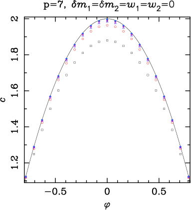
Figure 6: Estimates of the central charge for the ground state (with root configuration given by (72)) for $p=7$ ($Q\simeq 3.2469796$) as a function of the twist $\varphi$. We show the numerical solutions of the BAE for sizes $L=6$ (black $\square$), $L=12$ (red $\circ$), $L=18$ (navy blue $\triangle$), $L=24$ (pink $\lozenge$), $L=30$ (orange $\times$), $L=36$ (violet $\blacklozenge$), $L=42$ (dark gray $\blacksquare$), and $L=48$ (blue $\bullet$). The convergence towards the analytic formula $c=2-\frac{6p}{p-4}\left(\frac{\varphi}{\pi}\right)^{2}$ [cf. (66)], depicted as a black curve, is excellent.

As discussed in the previous section, the excitations above the ground state are obtained by creating ‘holes’ and ‘backscatterings’ in the Fermi seas of $x$ and $y$ (we shall not consider here the excitation obtained by forming 2-strings). Introducing the densities of holes $\rho^{h}$ and $\sigma^{h}$ (which play an analogous role as the densities of roots $\rho$ and $\sigma$), we can write the scattering equations in a matrix form

$$\left(\begin{array}[]{c}\rho+\rho^{h}\\ \sigma+\sigma^{h}\end{array}\right)\;=\;s+K\left(\begin{array}[]{c}\rho\\ \sigma\end{array}\right)\,.$$ (61)

The conformal weights of excitations indexed by the holes numbers $(\delta m_{1},\delta m_{2})$ and backscatterings $(w_{1},w_{2})$ are obtained (at zero twist) as [62]

$$\Delta_{\alpha}+\bar{\Delta}_{\alpha}\;=\;\frac{1}{4}(\delta m_{1},\delta m_{2})\left(1-K\right)\left(\begin{array}[]{c}\delta m_{1}\\ \delta m_{2}\end{array}\right)+(w_{1},w_{2})\left(1-K\right)^{-1}\left(\begin{array}[]{c}w_{1}\\ w_{2}\end{array}\right)\,,$$ (62)

where the label $\alpha$ denotes for the set of quantum numbers of a given excitation, and in $1-K$ the zero-frequency limit $\omega\to 0$ has to be taken, so

$$1-K\;=\;\left(\begin{array}[]{rr}2-\frac{\theta}{\pi}&-1-\frac{\theta}{\pi}\\ -1-\frac{\theta}{\pi}&2-\frac{\theta}{\pi}\end{array}\right)\,.$$ (63)

Therefore,

$$\Delta_{\alpha}+\bar{\Delta}_{\alpha} = \frac{1}{2}\left[\left(1-\frac{1}{p}\right)\left({\delta m_{1}}^{2}+{\delta m_{1}}^{2}\right)-\left(1+\frac{2}{p}\right){\delta m_{1}}{\delta m_{2}}\right]$$ (64)

$$\qquad\qquad+\frac{2}{3}\left({w_{1}}^{2}+{w_{1}}{w_{2}}+{w_{2}}^{2}\right)+\frac{2}{p-4}\left({w_{1}}+{w_{2}}\right)^{2}\,,$$

which can readily be checked numerically. Further, we also check numerically that introducing particle-hole excitations results in the following conformal weights with respect to the ground state of the untwisted $c=2$ theory

$$\Delta_{\alpha}+\bar{\Delta}_{\alpha} = \frac{1}{2}\left[\left(1-\frac{1}{p}\right)\left({\delta m_{1}}^{2}+{\delta m_{1}}^{2}\right)-\left(1+\frac{2}{p}\right){\delta m_{1}}{\delta m_{2}}\right]$$ (65)

$$\qquad+\frac{2}{3}\left({w_{1}}^{2}+{w_{1}}{w_{2}}+{w_{2}}^{2}\right)+\frac{2}{p-4}\left(w_{1}+w_{2}\right)^{2}$$

$$\qquad+\delta_{1}^{+}+\delta_{1}^{-}+\delta_{2}^{+}+\delta_{2}^{-}\,.$$

It is also of interest to study what happens to these excited states when a twist $\varphi$ is turned on. We therefore measure numerically the corresponding effective central charges, $c_{\alpha}=2-12\left(\Delta_{\alpha}+\bar{\Delta}_{\alpha}\right)$, as a function of the twist. Solving the corresponding BAE for sizes up to $L\sim 100$, we find the corresponding formula

$$c_{\alpha}(\varphi) = 2-6\left[\left(1-\frac{1}{p}\right)\left({\delta m_{1}}^{2}+{\delta m_{1}}^{2}\right)-\left(1+\frac{2}{p}\right){\delta m_{1}}{\delta m_{2}}\right]$$ (66)

$$\qquad-8\left({w_{1}}^{2}+{w_{1}}{w_{2}}+{w_{2}}^{2}\right)-\frac{24}{p-4}\left({w_{1}}+{w_{2}}\right)^{2}$$

$$\qquad-\frac{6p}{p-4}\frac{\varphi}{\pi}\left(\frac{\varphi}{\pi}+2(w_{1}+w_{2})\right)-12\left(\delta_{1}^{+}+\delta_{1}^{-}+\delta_{2}^{+}+\delta_{2}^{-}\right)\,.$$

An example is shown in figure 6, where we measure numerically the central charge associated with the ground state (72) as a function of the twist, and which shows an excellent agreement with the formula (66).

The exponents $\Delta_{\alpha},\bar{\Delta}_{\alpha}$ are measured with respect to the untwisted model with central charge $c=2$. Anticipating on the results of section 5.1.1, the exponents of the Potts model should instead be measured with the twisted central charge (73). We shall therefore consider the shifted exponents $h_{\alpha},\bar{h}_{\alpha}$,

$$h_{\alpha}+\bar{h}_{\alpha}\;=\;\Delta_{\alpha}+\bar{\Delta}_{\alpha}-\frac{2}{p(p-4)}\,.$$ (67)

Or, more precisely,

$$h_{\alpha}+\bar{h}_{\alpha} = \frac{1}{2}\left[\left(1-\frac{1}{p}\right)\left({\delta m_{1}}^{2}+{\delta m_{1}}^{2}\right)-\left(1+\frac{2}{p}\right){\delta m_{1}}{\delta m_{2}}\right]$$ (68)

$$\qquad+\frac{2}{3}\left({w_{1}}^{2}+{w_{1}}{w_{2}}+{w_{2}}^{2}\right)+\frac{2}{p-4}\left({w_{1}}+{w_{2}}\right)^{2}$$

$$\qquad+\delta_{1}^{+}+\delta_{1}^{-}+\delta_{2}^{+}+\delta_{2}^{-}$$

$$\qquad+\frac{p}{2(p-4)}\frac{\varphi}{\pi}\left(\frac{\varphi}{\pi}+2(w_{1}+w_{2})\right)-\frac{2}{p(p-4)}\,.$$

To disentangle $h_{\alpha}$ from $\bar{h}_{\alpha}$, we can further use the translational invariance of the system, implying that the TM commutes with the momentum operator. The latter can be written as a sum over Bethe integers,

$$P\;=\;\frac{2\pi}{L}\left(\sum_{i=1}^{m_{1}}2I_{j}+\sum_{k=1}^{m_{2}}2J_{k}\right)\,.$$ (69)

So we readily have, for the states of interest:

$$P_{\alpha} = \frac{2\pi}{L}\left[\left(\frac{2L}{3}-\delta m_{1}\right)w_{1}+\left(\frac{L}{3}-\delta m_{2}\right)w_{2}+\delta_{1}^{+}+\delta_{2}^{+}-\delta_{1}^{-}-\delta_{2}^{-}\right]$$ (70)

$$= 2\pi\left(\frac{2}{3}w_{1}+\frac{1}{3}w_{2}\right)+\frac{2\pi}{L}\left(\delta_{1}^{+}+\delta_{2}^{+}-\delta_{1}^{-}-\delta_{2}^{-}-\delta m_{1}w_{1}-\delta m_{2}w_{2}\right)\,.$$

In the continuum limit, the $\frac{1}{L}$-dependent part is related to the conformal spin $h_{\alpha}-\bar{h}_{\alpha}$, as

$$h_{\alpha}-\bar{h}_{\alpha}\;=\;\delta_{1}^{+}+\delta_{2}^{+}-\delta_{1}^{-}-\delta_{2}^{-}-\delta m_{1}w_{1}-\delta m_{2}w_{2}\,.$$ (71)

5 Critical content of the colouring problem

We will now restrict to the specific states observed in the Potts spectrum. This will lead to analytic expressions for the central charge, the thermal and magnetic exponents, and the watermelon exponents describing the propagation of several FK clusters. Combining this information will finally lead to the identification of the CFT describing vertex colourings of the triangular lattice.

5.1 Ground state ($k=0$) sector

5.1.1 Central charge.

As already explained, the ground state of the Potts model (namely, in the $k=0$ sector), can be found as an eigenstate in the zero magnetisation sector of the spin-one vertex model, at twist $\varphi=\theta$. In terms of Bethe roots, it simply corresponds to

$$(\delta m_{1},\delta m_{2})\;=\;(0,0)\,,\quad(w_{1},w_{2})\;=\;(0,0)\,,\quad\varphi\;=\;\theta\,.$$ (72)

From equation (66), we therefore directly read the corresponding central charge,

$$c\;=\;2-\frac{24}{p(p-4)}\,.$$ (73)

We have made an extensive numerical test of this formula by

• Direct diagonalisation of the TM for small values of $L=6,9,12$. In this case we were able to cover the whole interval $Q\in(2,4)$ in steps of size $10^{-3}$.

• Numerically solving the BAE for sizes $L=6,9,12,24,48,96$ with the right twist $\varphi=\theta$. Except for $L=6,9$, we could solve these equations in the smaller interval $Q\in[2.469,4)$, again in steps of size $10^{-3}$. Note that for $Q\in(2,B_{5})$, the root configurations contain one or more 2-strings. Furthermore, the higher the value of $L$, the larger the number of 2-strings that might appear in the configuration. This technical complication prevented us from studying the interval $(2,2.469)$ for $L\geq 12$ by solving the BAE. Indeed, for $L=6,9,12$ the results obtained from this method agree perfectly well with those obtained from the TM diagonalisation.

In particular, for each value of $Q\in[2.469,4)$, we computed the free energy $f_{L}(Q)$ for $L=6,12,24,48,96$. ($f_{9}(Q)$ was computed mainly for testing our methods.) We then performed the standard three-parameter fit based [cf. (35)] on the CFT Ansatz $f_{L}(Q)=f_{\text{bulk}}(Q)+\frac{\pi G}{6L^{2}}c(Q)+\frac{A}{L^{4}}$, using three consecutive values of the width, $L=L_{\text{min}},2L_{\text{min}},4L_{\text{min}}$, to obtain the unknowns $f_{\text{bulk}}(Q)$, $c(Q)$ and $A$. As a precaution against finite-size effects, we repeated the fits for three different values of $L_{\text{min}}$.

The values obtained for $f_{\text{bulk}}$ agree very well with those given by Baxter’s exact expression for regime IV (16), even though we are also computing the former values for $Q$ much less than $Q_{0}$ [cf. (19)], where the ground state of regime I is dominant. This vividly illustrates the fact—discussed at the end of section 2.4—that regimes I and IV coexist, in the sense that the scaling levels of either of them are well-defined by analytic continuation on the other side of $Q_{0}$.

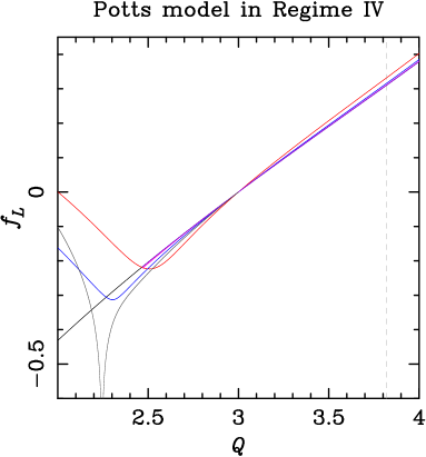
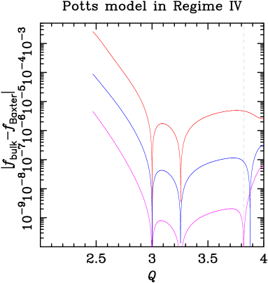
(a)	(b)

Figure 7: (a) Values of the free energies $f_{L}$ as a function of $Q$ for several values of the width: $L=6$ (red), $L=12$ (blue), $L=24$ (pink), $L=48$ (orange), and $L=96$ (violet). The dark-gray curve diverging at $Q\approx 2.224$ corresponds to $L=9$. The black curve corresponds to Baxter’s exact result (16). (b) Absolute difference $|f_{\text{bulk}}-f_{\text{Baxter}}|$ for the bulk free energy obtained from the three-parameter fit $f_{L}(Q)=f_{\text{bulk}}(Q)+\frac{\pi G}{6L^{2}}c(Q)+\frac{A}{L^{4}}$ with $L_{\text{min}}=6$ (red), $L_{\text{min}}=12$ (blue), and $L_{\text{min}}=24$ (pink).

In figure 7(a) we depict the raw data for $f_{L}(Q)$, as well as Baxter’s free energy (16), and in panel (b) we show the discrepancies between $f_{\text{bulk}}$ and $f_{\text{Baxter}}$ (16) in semi-logarithmic scale. The agreement is very good. This result shows that the ground state of regime IV can be analytically continued deep inside the regime I. We believe that this agreement can be extended to the range $2<Q\leq 4$, and we have made extensive tests to verify this claim. Indeed we have followed the free-energy level $f_{L}$ which is dominant at $Q=4$ (i.e., the ground state of regime IV) by analytic continuation to smaller $Q$—using both direct diagonalisation of the TM for small $L$, and numerical BA computations for larger $L$—and found it to have the following features:

• If $L\in 6{\mathbb{N}}$, the level $f_{L}$ follows Baxter’s $g_{2}$ closely down to some value $Q_{\rm min}(L)>2$ where $f_{L}(Q)$ has a minimum. For $Q<Q_{\rm min}(L)$, $f_{L}$ breaks away from $g_{2}$. However, for $L=9$ (see figure 7(a)), although the behaviour is similar, we find a divergence at $Q_{\rm div}(9)\approx 2.244$, rather than a minimum. Therefore we expect parity effects, so in our main fits we will only include even values of $L$.

• There is good evidence that $Q_{\rm min}(L)\to 2$ as $L\to\infty$ for $L\in 6{\mathbb{N}}$. We also conjecture that $Q_{\rm div}(L)\to 2$ as $L\to\infty$ for $L$ being an odd multiple of 3.

• Right at $Q=2$, we find that $f_{L}$ takes a finite value that, at least for $L=6,9,12$ decreases as $L$ increases. If we fit the corresponding $f_{L}(2)$ values to the standard CFT 3-parameter Ansatz, we obtain $f_{\text{bulk}}(2)\approx-0.2570$, which is still larger than Baxter’s value $g_{2}(2)\approx-0.4315231$.

These observations indicate that $f_{L}\to g_{2}$ as $L\to\infty$ on the interval $Q\in(2,4]$, but the convergence is not uniform. This feature is responsible of the ‘largest’ discrepancies observed for $Q\lessapprox B_{5}$. Indeed, for $Q\to 2^{+}$ the central charge (73) diverges, signaling the break-down of regime IV. On the other hand, we have found no evidence of regime IV levels whose analytic continuation converge to $g_{2}$ for $0\leq Q<2$. Since $g_{2}$ is analytic on the whole interval $0\leq Q\leq 4$, it is possible that it serves as the ground state of yet another regime (and a different CFT) for $Q\in[0,2)$, but further examination of this issue is beyond the scope of the present paper.

A further noteworthy feature concerns the value of the analytic continuation of regime IV’s ground state to $Q=3$. We find that $f_{L}(3)=0$ exactly for any $L$. This should be compared with the simple fact that a triangular-lattice strip with cylindrical boundary conditions and width $L$ a multiple of 3 is uniquely 3-colourable modulo global colour permutations (i.e. $Z_{G}(3,-1)=3!$). Therefore regime IV captures an essential feature of the colouring problem at $Q=3$.

Finally, in figure 7(b) we observe that the convergence of $f_{L}$ to $g_{2}$ is noticeable slower close to $Q=4$. This is probably due to the usual logarithmic corrections at $Q=4$, well-known in the Potts-model context.

The reader might worry if all of this does not contradict the simple observation that $Z=0$ for $Q=2$, since a triangular lattice manifestly does not admit a proper vertex 2-colouring. As a matter of fact, there is no problem, because at $Q=2$ massive cancellations of TM eigenvalues will occur, due to three distinct mechanisms:

1. Some of the eigenvalues are simply zero;

2. Other eigenvalues have a zero amplitude in the decomposition of the Markov trace [35];

3. Some eigenvalues are equal up to a sign, and their combined amplitude summed over the various sectors of the TM is zero.

The end result is that $Z=0$ indeed, despite the existence of finite eigenvalues, and we have checked this explicitly for small $L$.

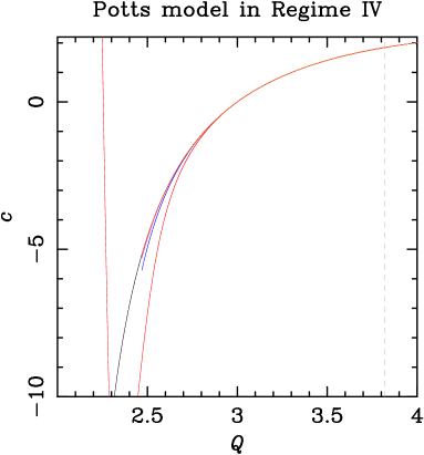
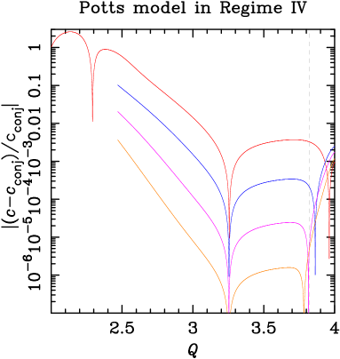
(a)	(b)

Figure 8: (a) Values of the central charge $c$ obtained by performing the 2-parameter fit $f_{L}(Q)-f_{\text{Baxter}}(Q)=\frac{\pi G}{6L^{2}}c(Q)+\frac{A}{L^{4}}$ for $L_{\text{min}}=6$ (red), $L_{\text{min}}=12$ (blue), $L_{\text{min}}=24$ (pink), and $L_{\text{min}}=48$ (orange). The black curve shows the conjectured value (73). Note that the fits cover the interval $(2,4)$ for $L_{\text{min}}=6$, while they cover the smaller interval $[2.469,4)$ for the other values. (b) Relative difference between the estimated central charge and the conjecture (73) in semi-logarithmic scale.

Now that the agreement of $f_{\text{bulk}}$ with $f_{\text{Baxter}}$ has been firmly established, we can obtain more precise estimates for the central charge $c$ by performing fits with only two parameters, $c(Q)$ and $A$, using the CFT Ansatz $f_{L}(Q)-f_{\text{Baxter}}(Q)=\frac{\pi G}{6L^{2}}c(Q)+\frac{A}{L^{4}}$ and the exact result (16). Accordingly, we fitted our data for two consecutive values of $L$, namely $L=L_{\text{min}},2L_{\text{min}}$, for different values of $L_{\text{min}}$. The results are depicted in figure 8. The agreement between the numerical estimates for the central charge and conjecture (73) is excellent, including for $Q<Q_{0}$. There is indeed good evidence that $c$ converges to (73) for all $Q\in(2,4]$, but once again the convergence is not uniform; note in particular that $c\to-\infty$ as $Q\to 2^{+}$, whereas $f_{\text{Baxter}}$ stays finite at $Q=2$.

At $Q=3$, we find that $c=0$ exactly for any $L$, as expected from the total absence of finite-size effects noticed above. This value $c=0$ agrees with the obvious non-critical nature of the 3-colouring problem. On the other hand, close to $Q=4$, the observed larger discrepancies are again due to logarithmic corrections.

5.1.2 Thermal exponent.

It is now interesting to further consider the excited states in the $k=0$ sector, and in particular the first of these, which in the continuum limit corresponds to the thermal field. Although the corresponding root configuration is highly unstable under variations of the twist, we can nevertheless describe its analytic continuation at zero twist, which is made of

• $\frac{2L}{3}-2$ real roots.

• $\frac{L}{3}-2$ roots with imaginary part $\frac{\pi}{2}$.

• Two degenerate 2-strings, with zero real part and the same imaginary part.

Figure 9: Configurations of the Bethe roots associated with the ground state in regime IV, as a function of the twist parameter. For $\varphi<\pi$, it is described by a Fermi sea of $\frac{2L}{3}$ real roots (black dots) and a Fermi sea of $\frac{L}{3}$ roots with imaginary part $\frac{\pi}{2}$ (white dots). As $\varphi\to\pi^{-}$, the real parts of the rightmost roots of each Fermi sea go to $+\infty$. As $\varphi$ crosses $\pi$, these two roots form one 2-string (black squares). The same process occurs once again as $\varphi\to 2\pi^{-}$, resulting in a configuration with two degenerate 2-strings at $\varphi=2\pi$. Although on the picture these are distinct, it should be kept in mind that the corresponding roots actually coincide two by two.

Let us now go back to the ground state configuration (72), and try to follow it continuously as the twist is increased. The evolution of the Bethe roots from $\varphi=0$ to $\varphi=2\pi$ is depicted schematically in figure 9. It is seen that the root configurations encounters qualitative changes, namely, the formation of 2-strings, as $\varphi$ crosses multiples of $\pi$. More precisely, the root configuration associated with the thermal exponent at $\varphi=0$ actually corresponds to the continuation of the ground state configuration to $\varphi=2\pi$. The corresponding conformal weight can therefore be obtained straightforwardly by analytic continuation of the conformal weight for the twisted ground state (this is after all exactly the same as what was observed in regime I, see section 4.2) .

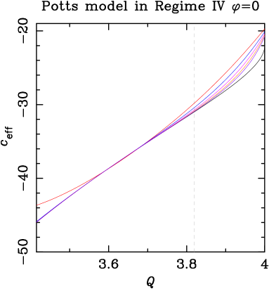
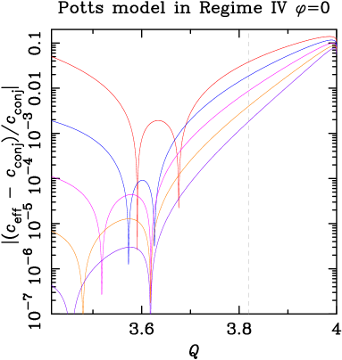
(a)	(b)

Figure 10: Fits for the subdominant free energy in regime IV at zero twist. (a) Values of the effective central charge $c_{\text{eff}}$ obtained by performing the 2-parameter fit $f_{2,L}(Q)-f_{\text{Baxter}}(Q)=\frac{\pi G}{6L^{2}}c_{\text{eff}}(Q)+\frac{A}{L^{4}}$ for $L_{\text{min}}=12$ (red), $L_{\text{min}}=24$ (blue), $L_{\text{min}}=48$ (pink), $L_{\text{min}}=96$ (orange), and $L=192$ (violet). The black curve shows the conjectured value (74). (b) Relative difference between the estimated central charge and the conjecture (74) in semi-logarithmic scale.

To check this assumption, we have solved numerically the zero-twist BAE associated with the first excited state continued to $\varphi=0$ (remember that the true level present in the Potts model, namely at a twist $\varphi=\theta$, corresponds to a highly unstable configuration of roots, whose numerical study does not appear feasible) for sizes up to $L=384$ in the interval $Q\in(B_{8},4)$. For each value of $Q$, we computed the corresponding free energy $f_{2,L}(Q)$ for $L=12,24,48,96,192$, and $384$. We then performed the standard three-parameter fit $f_{2,L}(Q)=f_{\text{bulk}}(Q)+\frac{\pi G}{6L^{2}}c_{\text{eff}}(Q)+\frac{A}{L^{4}}$ for three consecutive values of the width $L=L_{\text{min}},2L_{\text{min}},4L_{\text{min}}$. As for the leading eigenvalue, the values obtained for $f_{\text{bulk}}$ agree very well with those given by Baxter’s exact expression for regime IV (16). A better estimate for $c_{\text{eff}}$ is obtained by using the 2-parameter CFT Ansatz $f_{2,L}(Q)-f_{\text{Baxter}}(Q)=\frac{\pi G}{6L^{2}}c_{\text{eff}}(Q)+\frac{A}{L^{4}}$, and two consecutive values of $L=L_{\text{min}},2L_{\text{min}}$. The results are depicted in figure 10, and agree with the conjecture

$$c_{\text{eff}}\;=\;-22-\frac{96}{p-4}\,,$$ (74)

that is, precisely the expression obtained from (66) at $\delta m_{1}=\delta m_{2}=w_{1}=w_{2}=\delta_{1}^{\pm}=\delta_{2}^{\pm}=0$ for a twist $\varphi=2\pi$. The agreement between the numerical estimates for the effective central charge and conjecture (74) is excellent, especially for values of $Q$ far away from $4$. Close to $Q=4$, we should expect logarithmic corrections as those shown in figure 8, implying a slower convergence towards (74).

From there we assume, as in regime I, that the subleading eigenlevels in the $k=0$ sector are obtained from the ground state level by taking twists of the form $\varphi=\theta+2\pi j$, leading to effective central charges

$$c_{\text{eff},j}\;=\;2-\frac{24}{p(p-4)}\left(1+jp\right)^{2}\,,$$ (75)

and therefore to conformal weights of the form

$$h_{j}+\bar{h}_{j}\;=\;\frac{1}{12}\left(c-c_{\text{eff},j}\right)\;=\;\frac{2j}{p-4}\left(2+jp\right)\,.$$ (76)

Among these, the two least irrelevant correspond to $j=1$ and $j=-1$, namely

$$x_{T}\;=\;h_{-1}+\bar{h}_{-1}\;=\;2+\frac{4}{p-4}\,,\qquad x^{\prime}_{T}\;=\;h_{1}+\bar{h}_{1}\;=\;2+\frac{12}{p-4}\,.$$ (77)

5.1.3 Magnetic exponent.

As explained in section 3.4, the magnetic exponent is associated to the scaling of the leading TM eigenvalue in sector $k=0$, with twist $\frac{\varphi}{2}=\frac{\pi}{2}$. From our observations in section 5.4, we know that this eigenvalue can be associated with the quantum numbers

$$(\delta m_{1},\delta m_{2})\;=\;(0,0)\,,\quad(w_{1},w_{2})\;=\;\left(-\frac{1}{2},\frac{1}{2}\right)\,,\quad\varphi\;=\;0\,,$$ (78)

and therefore with an effective central charge

$$c_{\text{eff}}=0\,.$$ (79)

From there, we directly read off the magnetic exponent,

$$x_{H}\;=\;\frac{1}{12}\left(c-c_{\text{eff}}\right)\;=\;\frac{1}{6}-\frac{2}{p(p-4)}\,.$$ (80)

5.2 Even $k$ sectors.

For instance we study the sector $k=2$, for $Q=3.99$, and $L=9$. The eigenenergies given are of the form $f_{i}=\frac{1}{L}\log\Lambda_{i}$, where $\Lambda_{i}$ are the TM eigenvalues:

$$\begin{array}[]{cccl}f_{0}&=&0.356989&\quad(\delta m_{1},\delta m_{2})=(1,1)\,,(w_{1},w_{2})=(0,0)\,,\varphi=0\\ f_{1}=f_{2}&=&0.343760&\quad(\delta m_{1},\delta m_{2})=(1,1)\,,(w_{1},w_{2})=(\pm 1,0)\,,\varphi=\mp\pi\\ f_{3}=f_{4}&=&0.321961&\quad(\delta m_{1},\delta m_{2})=(1,1)\,,(w_{1},w_{2})=(\pm 1,0)\,,\varphi=0\\ f_{5}=f_{6}&=&0.316346&\quad(\delta m_{1},\delta m_{2})=(2,2)\,\text{+ one 2-string}\\ f_{7}=f_{8}&=&0.314850&\quad(\delta m_{1},\delta m_{2})=(1,1)\,,(w_{1},w_{2})=(0,0)\,,\delta_{1}^{\pm}=1\,,\varphi=0\\ f_{9}=f_{10}&=&0.309532&\quad(\delta m_{1},\delta m_{2})=(1,1)\,,(w_{1},w_{2})=(\pm 1,\pm 1)\,,\varphi=0\\ f_{11}=f_{12}&=&0.304716&\quad(\delta m_{1},\delta m_{2})=(1,1)\,,(w_{1},w_{2})=(\pm 2,0)\,,\varphi=\mp 2\pi\\ f_{13}=f_{14}&=&0.302223&\quad(\delta m_{1},\delta m_{2})=(1,1)\,,(w_{1},w_{2})=(\pm 1,0)\,,\delta_{1}^{\mp}=1\,,\varphi=0\\ &\ldots&&\\ \end{array}$$

(when no mention is made of the $\delta_{1},\delta_{2}$ numbers, these are equal to zero).

From this example as well as further examination of the $k=4,6,8$ cases, we see that the least excited states making up the even $k\geq 2$ sectors are associated with

$$\delta m_{1}\;=\;\delta m_{2}\;=\;\frac{k}{2}\,,\quad w_{1},w_{2}\in\mathbb{Z}\,,\quad\varphi\;=\;{n\pi}\,,\quad n\in\mathbb{Z}\,.$$ (81)

From (68)/(71), we find the corresponding conformal spins

$$h-\bar{h}=-\frac{1}{2}k\left(w_{1}+w_{2}\right)\,,$$ (82)

which indeed assume integer values, while the conformal weights are found to be

$$h = \frac{\left[k(p-4)-(2n+2(w_{1}+w_{2}))p\right]^{2}-16}{16p(p-4)}+\frac{1}{12}\left(3kn+\left(w_{2}-w_{1}\right)^{2}\right)$$ (83)

$$\bar{h} = \frac{\left[k(p-4)-(2n+2(w_{1}+w_{2}))p\right]^{2}-16}{16p(p-4)}$$ (84)

$$\qquad\qquad+\frac{1}{12}\left(3k(n+2w_{1}+2w_{2})+\left(w_{2}-w_{1}\right)^{2}\right)\,.$$

5.3 Odd $k\geq 3$ sectors.

We here specialize to odd sectors with $k\geq 3$, as the $k=1$ case is a bit particular, as we shall see in the next section. Similarly, for $k=3$, $Q=3.99$, and $L=9$, the lowest-lying levels are the following:

$$\begin{array}[]{cccl}f_{1}=f_{2}&=&0.316285&\quad(\delta m_{1},\delta m_{2})=(2,1)\,,(w_{1},w_{2})=(\pm\frac{1}{2},0)\,,\varphi=0\\ f_{3}=f_{4}&=&0.313692&\quad(\delta m_{1},\delta m_{2})=(2,1)\,,(w_{1},w_{2})=(\pm\frac{1}{2},0)\,,\varphi=\mp\frac{2\pi}{3}\\ f_{5}=f_{6}&=&0.290629&\quad(\delta m_{1},\delta m_{2})=(2,1)\,,(w_{1},w_{2})=(\pm\frac{1}{2},0)\,,\varphi=0\,,\delta_{1}^{\mp}=1\\ f_{7}=f_{8}&=&0.288732&\quad(\delta m_{1},\delta m_{2})=(2,1)\,,(w_{1},w_{2})=(\pm\frac{1}{2},\mp 1)\,,\varphi=\pm\frac{4\pi}{3}\\ &\ldots&&\\ \end{array}$$

For $k=5$, $Q=3.99$, and $L=9$, we find

$$\begin{array}[]{cccl}f_{1}=f_{2}&=&0.239272&\quad(\delta m_{1},\delta m_{2})=(3,2)\,,(w_{1},w_{2})=(0,\pm\frac{1}{2})\,,\varphi=\mp\frac{4\pi}{5}\\ f_{3}=f_{4}&=&0.229800&\quad(\delta m_{1},\delta m_{2})=(3,2)\,,(w_{1},w_{2})=(0,\pm\frac{1}{2})\,,\varphi=\mp\frac{2\pi}{5}\\ f_{5}=f_{6}&=&0.224099&\quad(\delta m_{1},\delta m_{2})=(3,2)\,,(w_{1},w_{2})=(\mp 1,\pm\frac{1}{2})\,,\varphi=\mp\frac{2\pi}{5}\\ f_{7}=f_{8}&=&0.222247,&\quad(\delta m_{1},\delta m_{2})=(3,2)\,,(w_{1},w_{2})=(0,\pm\frac{1}{2})\,,\varphi=\mp\frac{4\pi}{5}\,,\delta_{1}^{\pm}=1\\ f_{9}=f_{10}&=&0.220503&\quad(\delta m_{1},\delta m_{2})=(3,2)\,,(w_{1},w_{2})=(\pm 1,\pm\frac{1}{2})\,,\varphi=\mp\frac{2\pi}{5}\,,\delta_{1}^{\mp}=1\\ &\ldots&&\\ \end{array}$$

In the latter case states corresponding to $\varphi=0$, for instance $(\delta m_{1},\delta m_{2})=(3,2)\,,(w_{1},w_{2})=(0,\pm\frac{1}{2})\,,\varphi=0$ are also found, but lie deeper in the Potts spectrum.

From these examples, as well as further examination of the $k=7$ and $k=9$ cases, we see that the least excited states making up the odd $k>1$ sectors are associated with

$$\delta m_{1}=\frac{k+1}{2}\,,\quad\delta m_{2}=\frac{k-1}{2}\,,\quad w_{1}=v_{1}+\frac{k-1}{4}\,,\quad w_{2}=v_{2}+\frac{k+1}{4}\,,\quad\varphi=\frac{2n\pi}{k}\,,$$ (85)

where $v_{1}$, $v_{2}$ and $n$ take integer values.

From (68)/(71), we find the corresponding conformal spins

$$h-\bar{h}=\frac{1}{4}\left(1-k^{2}+2(v_{2}-v_{1})-2k(v_{1}+v_{2})\right)\,,$$ (86)

which indeed assumes integer values, while the conformal weights are found to be

$$h = \frac{\left[k(p-4)-(k+4\frac{n}{k}+2(v_{1}+v_{2}))p\right]^{2}-16}{16p(p-4)}$$ (87)

$$+\frac{1}{12}\left(6n+\left(v_{2}-v_{1}+2\right)^{2}\right)$$

$$\bar{h} = \frac{\left[k(p-4)-(k+4\frac{n}{k}+2(v_{1}+v_{2}))p\right]^{2}-16}{16p(p-4)}$$ (88)

$$\qquad\qquad+\frac{1}{12}\left(3k^{2}+6(n+kv_{1}+kv_{2})+\left(v_{2}-v_{1}-1\right)^{2}\right)$$

5.4 $k=1$ sectors.

As we mentioned in section 3.4, the $k=1$ case is a bit particular, in that there are two ways to have one propagating cluster in the vertical direction, namely it may or may not be allowed to wrap around the cylinder. Let us study these two cases independently:

5.4.1 Cluster allowed to wrap around the cylinder.

Forbidding loops on the kagome lattice to wrap around the cylinder amounts to giving such loops a weight $0$, and therefore to fixing a twist $\frac{\varphi}{2}=\frac{\pi}{2}$.

Indeed, the largest eigenvalue of the FK TM in this sector is found in the zero-magnetisation sector of the vertex model at twist $\varphi=\pi$. Alternatively, it can be obtained at zero twist from the following set of Bethe parameters

$$(\delta m_{1},\delta m_{2})\;=\;(0,0)\,,\quad(w_{1},w_{2})\;=\;\left(-\frac{1}{2},\frac{1}{2}\right)\,,\quad\varphi\;=\;0\,.$$ (89)

5.4.2 Cluster not allowed to wrap around the cylinder.

Forbidding the propagating cluster to wrap around the cylinder amounts to fixing one through-line in the O$(n)$ model. Therefore we expect to find the corresponding leading eigenvalues in the sector of magnetisation $m=1$.

This is the case as, for instance, we find for $Q=3.99$ and $L=6$ the following set of leading eigenenergies: The first dominant states form complex quartet

$$\begin{array}[]{ccc}f_{1}&=&0.302084+0.355356\,\mathrm{i}\\ f_{2}&=&0.302084-0.355356\,\mathrm{i}\\ f_{3}&=&0.302084+0.342775\,\mathrm{i}\\ f_{4}&=&0.302084-0.342775\,\mathrm{i}\end{array}$$

and the next states are given by

$$\begin{array}[]{cccl}f_{5}=f_{6}&=&0.272659&\quad(\delta m_{1},\delta m_{2})=(2,-1)\,,(w_{1},w_{2})=\left(\pm\frac{1}{2},0\right)\,,\varphi=0\\ f_{7}=f_{8}&=&0.269606&\quad(\delta m_{1},\delta m_{2})=(2,1)\text{+ one 2-string}\,,\varphi=0\\ f_{9}&=&0.227715&\quad(\delta m_{1},\delta m_{2})=(2,-1)\,,(w_{1},w_{2})=(0,0)\,,\varphi=0,\\ &&&\quad\qquad\delta_{1}^{+}=\delta_{1}^{-}=\frac{1}{2}\\ &\ldots&&\end{array}$$

The complex quartet, as we understand it, is associated to very peculiar root configurations. From observations at $L=6$ and $L=9$, we see that the corresponding root configurations are made of:

• $\frac{2L}{3}-1$ roots with imaginary parts very close to $0$.

• $\frac{L}{3}-1$ roots with imaginary part very close to $\frac{\pi}{2}$.

• One root with imaginary part very close to $\frac{\pi}{4}$.

Such configurations are rather odd, and out of the scope of our analytical solution. In addition, we were unfortunately unable to solve the corresponding BAE numerically for large system sizes, and therefore we could not access the corresponding conformal weights.

5.5 Identification of the CFT

The central charge (73) is the analytic continuation to any real $p>4$ of that of the $S_{3}$-invariant minimal models studied by Fateev and Zamolodchikov [63, 64], which can alternatively be formulated as the conformal cosets

$$\frac{SU(2)_{4}\times SU(2)_{p-6}}{SU(2)_{p-2}}\,,$$ (90)

defined for integer values of $p\geq 6$.

The corresponding sets of conformal weights are known [63, 64] to be parametrised by two integers, $1\leq r\leq p-5$, $1\leq s\leq p-2$, and read

$$h_{r,s}\;=\;\frac{\left[rp-s(p-4)\right]^{2}-16}{16p(p-4)}+\frac{1-\cos^{4}\left(\pi\frac{r-s}{4}\right)}{12}\,.$$ (91)

In addition there is another series of primary fields, with conformal weights

$$h^{\prime}_{r,s}\;=\;h_{r,s}+\frac{1+\sin^{2}\left(\pi\frac{r-s}{4}\right)}{3}+\delta_{r,1}\delta_{s,1}+\delta_{r,1}\delta_{s,2}+2\delta_{r,2}\delta_{s,1}\,.$$ (92)

Both (91) and (92) can be written under the form $h_{r,s}(h^{\prime}_{r,s})=\frac{\left[rp-s(p-4)\right]^{2}-16}{16p(p-4)}+\delta h_{r,s}$, where $\delta h_{r,s}$ encodes the sector of the associated $S_{3}$ symmetry [64], and can be understood in the framework of a generalized CG construction as a boundary twist term [65] (this is analogous to the Neveu–Schwartz and Ramond sectors in supersymmetric CFTs, encoding the periodic or antiperiodic boundary conditions for the fermionic field [66]).

Let us now compare the conformal spectrum identified in regime IV with the exponents (91)/(92).

5.5.1 Thermal exponents.

In section 5.1.2, we have identified a series of subleading exponents, $h_{j}+\bar{h}_{j}$, given by (76). These exponents have zero momentum (in agreement with the fact that thermal fields should not break the translational symmetry), and therefore

$$h_{j}\;=\;\bar{h}_{j}\;=\;\frac{j}{p-4}\left(2+jp\right)\,.$$ (93)

These are readily identified as the dimensions $h_{r,s}$ in (91), with $r=4j+1$, and $s=1$.

5.5.2 Magnetic exponent.

In section 5.1.3, we have identified the magnetic exponent as (80). The latter cannot be written in terms of the table $h_{r,s}$ ($h^{\prime}_{r,s}$) with fixed, $p$-independent values of $r,s$. Instead, we find that it coincides with $x_{H}=h_{r,s}+\bar{h}_{r,s}=2h_{r,s}$, with

$$r\;=\;\frac{p-4}{2}\,,\quad s\;=\;\frac{p}{2}\,.$$ (94)

The fact that these indices are $p$-dependent and half-integer is not too surprising. Indeed, the magnetic exponent for the usual critical $Q$-state Potts model has similar features, since it can be written $h_{\frac{p-1}{2},\frac{p+1}{2}}$, where $p$ here denotes the minimal model index.

5.5.3 Even $k$ sectors.

In section 5.2, we have identified the leading conformal weights in the sectors with even $k\geq 2$ as given by eqs. (83)/(84). Note that the expressions for $h$ and $\bar{h}$ can be recovered from each other by setting $(w^{\prime}_{1},w^{\prime}_{2})=(-w_{1},-w_{2}),n^{\prime}=n+2w_{1}+2w_{2}$, so we only focus on the former, namely (83). The first term takes the form $\frac{\left[rp-s(p-4)\right]^{2}-16}{16p(p-4)}$, with $r=2n+2(w_{1}+w_{2})$, and $s=k$. Focusing on the most relevant state, namely that with $n=w_{1}=w_{2}=0$, the second term vanishes, and we recover for $k\equiv 0\pmod{4}$ an exact correspondence with the exponents (91), for which the term $\delta h_{r,s}$ is zero. This state has zero conformal spin and scaling dimension

$$x_{k}\;=\;h+\bar{h}\;=\;\frac{k^{2}(p-4)}{8p}-\frac{2}{p(p-4)}\,.$$ (95)

5.5.4 Odd $k$ sectors.

In section 5.3, we have identified the leading conformal weights in the sectors with even $k\geq 2$ as given by eqs. (87)/(88). As in the $k$ even case, the expressions for $h$ and $\bar{h}$ can be recovered from each other by a relabeling of the indices, namely $(w^{\prime}_{1},w^{\prime}_{2})=(-w_{1},-w_{2}),n^{\prime}=n+k(w_{1}+w_{2})$, so once again we only focus on the former, namely (87). The first term takes the form $\frac{\left[rp-s(p-4)\right]^{2}-16}{16p(p-4)}$, with $r=k+\frac{4n}{k}+2(v_{1}+v_{2})=\frac{4n}{k}+2(w_{1}+w_{2})$, and $s=k$. In particular, we notice that fractional values of $r$ are allowed in this case. It is also noticeable that contrarily to the case of $k$ even, no well-definite set of values of the parameters $v_{1},v_{2},n$ seems to give rive to a least irrelevant state.

5.6 Physical conclusions

The $Q$-colouring problem of the triangular lattice $G$ is defined sensu stricto only for $Q\in\mathbb{N}$. We have studied here its analytic continuation, in the form of the chromatic polynomial $\chi_{G}(Q)$, defined for $Q\in\mathbb{R}$. Within the critical range $0\leq Q\leq 4$, two distinct regimes (that we have called regimes I and IV) were identified [17], and we have shown that the ground state and scaling levels of either regime are well-defined regardless of considerations [18] about which ground state is dominant in absolute terms. In particular, regime I can be defined for $0\leq Q<4$, and regime IV makes sense for (at least) $2<Q\leq 4$.

We now substantiate our claims—first made in section 2.4—that regime IV is in fact the correct analytic continuation of the colouring problem. To this end, we show that this regime has the correct physical properties of a colouring problem for $Q=4$ and $Q=3$, and that its break-down in the limit $Q\to 2^{+}$ can again be motivated by properties of the colouring problem.

The $Q=4$ vertex colourings of the triangular lattice are equivalent to vertex 3-colourings of the kagome lattice and to edge 3-colourings of the honeycomb lattice [68, 69]. The latter problem has been studied in its own right [68] and, more generally, as the special case $n=2$ of the O($n$)-type fully-packed loop (FPL) model on the hexagonal lattice [70, 71]. The ground state free energy of these problems agree [17, 68, 70] and is given by (16), and since the formulation in terms of 3-edge colourings of the honeycomb lattice involves only real, non-negative Boltzmann weights [68], the Perron-Frobenius theorem ensures that (16) correctly gives the entropy of vertex 4-colourings of the triangular lattice.

A two-dimensional height mapping for the O($n$) FPL model was given in [71], and it was shown that the continuum limit is described by a Liouville field theory (or two-component CG) involving two compactified bosons with an $n$-dependent radius. For $n=2$ this reduces to two free bosons, so the central charge is $c=2$ in agreement with our result (73) for $Q=4$ ($p\to\infty$). A slightly different two-dimensional height mapping was given directly for the 4-colouring problem in [69]. The critical exponent $\eta=2x_{H}=\frac{1}{3}$ was also derived and checked numerically in [69], in agreement with our result (80) that gives $x_{H}=\frac{1}{6}$ for $Q=4$. This provides a couple of convincing checks that our continuum description is indeed that of the combinatorial colouring problem.

We next turn to the case $Q=3$. Even though this is less than $Q_{0}$ [see (19)], we claim that regime IV still correctly describes the physical colouring problem. It is easy to see that each of the three sublattices must have a constant colour, so $Z=3!$ for any size $L\in 3\mathbb{N}$, and this is compatible with our observation, made in section 4.4, that $f_{L}(3)=0$. A further confirmation comes from the magnetic exponent. Since there is a perfect ordering on each sublattice, the (staggered) two-point function is constant, so that $x_{H}=0$. This indeed agrees with (73) for $Q=3$ ($p=6$).

Finally, consider the limit $Q\to 2^{+}$. It is obviously not possible to colour an elementary triangular face with only two colours, but this does not imply that the ground-state free energy must diverge in this limit, because the cancellation mechanisms mentioned in section 4.4 are at play at $Q=2$. Indeed the regime IV expression (16) stays finite in this limit. However, the central charge (73), and all critical exponents derived above contain a pole at $Q=2$ ($p=4$), which is concomitant with the break-down of the colouring interpretation. On the other hand, it is possible to shift the ground-state energy by an infinite amount, so as to obtain a well-defined $Q=2$ theory in which each elementary face of the lattice contains precisely one frustrated edge (i.e., that is adjacent to two equally coloured spins). This defines the so-called zero-temperature Ising antiferromagnet, which possesses a critical ground-state ensemble corresponding to a $c=1$ CFT of one free boson [72, 73, 74]. It seems an appealing idea that this CFT should be (infinitely deeply) buried inside regime IV, but we have not investigated this question in details.

Further support that the critical colouring problem is described by regime IV for $2<Q\leq 4$ is provided by the RSOS representation to be described in section 6.

It is worth noticing that the results found in this paper favour Baxter’s value [18] for $Q_{0}$ [cf. (19)] against the alternative value $2+\sqrt{3}$ suggested in [10, section 6]. Furthermore, this conclusion may be a signal that Baxter’s eigenvalue $g_{1}$ (15) plays no role inside the critical region of the phase diagram in the complex $Q$-plane of the triangular-lattice chromatic polynomial (as it was investigated in [10]). Notice that even though $g_{1}$ is not defined for any real $Q\in(0,4)$, it is well defined when ${\rm Im}\,(Q)\neq 0$.

Before closing this section, we notice that our results for regime IV also have implications for the phase diagram in the $(Q,v)$ plane, outside the chromatic line $v=-1$. According to (77), the thermal perturbation of the ground state in regime IV is irrelevant for all $Q<4$. Therefore the part of the chromatic line where regime IV is dominant—that is, $Q_{0}<Q<4$—is attractive under the renormalisation group. We conclude that the small ‘bubble’ in figure 2, which is delimited by the bifurcation point $T$, the two branches of $v_{+}$ and the vertical line $Q=4$, is in the universality class of regime IV.

6 Connection with RSOS models and anyonic chains

In section 2.2 we discussed that at the Beraha numbers, $Q=B_{k}$, all of the unphysical regime I cancels out of the partition function. What remains is a purely local model encompassing regime IV. This local model is conveniently formulated as a restricted solid-on-solid (RSOS) height model, which has independent interest because of its relation with anyonic spin chains.

6.1 The RSOS model associated with the Izergin-Korepin vertex model

In section 3, we have explained how the colouring problem on the triangular lattice could be mapped onto an appropriately twisted version of the IK model, which can be viewed as a spin-1 vertex model: the degrees of freedom on each lattice edge are vectors in spin-1 representations of the quantum group $U_{\mathfrak{q}}(sl_{2})$, where $\mathfrak{q}=\mathrm{e}^{i\frac{\theta}{2}}=\mathrm{e}^{i\frac{\pi}{p}}$. These representations can at first stage be understood in the same way as classical $SU(2)$ representations, and the interaction between two edges at a vertex of the square lattice can therefore be decomposed into projectors on the spin $0$, spin $1$ and spin $2$ representations, namely

$$\leavevmode\hbox to45.62pt{\vbox to61.76pt{\text{[drawing]}}}\quad\propto\quad\left(P_{2}\right)_{ab}^{cd}+\frac{\sin\left(\theta+\frac{u}{2}\right)}{\sin\left(\theta-\frac{u}{2}\right)}\left(P_{1}\right)_{ab}^{cd}+\frac{\cos\left(\frac{3\theta}{2}+\frac{u}{2}\right)}{\sin\left(\frac{3\theta}{2}-\frac{u}{2}\right)}\left(P_{0}\right)_{ab}^{cd} a b c d a b c d$$ (96)

(for convenience the lattice has been rotated by $45^{\circ}$ with respect to the figures in section 3).

As we will now explain, this allows for a reintepretation of the model in terms of integer heights living on the faces of the square lattice (viz. vertices of the dual square lattice, shown in green in the following figure), namely in terms of an interaction-round-a-face (IRF) or solid-on-solid (SOS) model. The construction is adapted from the seminal work of Pasquier in the case of spin-$\frac{1}{2}$ models [37], and can be summed up as follows (for more details see [58]):

the $j_{i}$ and $j^{\prime}_{i}$ living on the nodes of the square lattice are (half)-integers encoding the representations of $U_{\mathfrak{q}}(sl_{2})$, and which must thus be compatible with the $U_{\mathfrak{q}}(sl_{2})$ fusion rules: for instance, if representations $j_{i}$ and $j_{i+1}$ are separated by a lattice edge (carrying a spin-1 representation), $j_{i+1}$ must belong to the fusion product $j_{i}\times 1$.

The action on the projectors $P_{0},P_{1},P_{2}$ on a given face of the dual lattice, specified by a set of heights $j_{i-1},j_{i},j_{i+1},j^{\prime}_{i}$, is worked out by a change of basis which makes use of the quantum analog of Wigner’s 6$j$ symbols and can be represented as follows :

$$\leavevmode\hbox to133.01pt{\vbox to50.78pt{\text{[drawing]}}}\;=\;\sum_{J}\left\{\begin{array}[]{ccc}j_{i-1}&1&j_{i}\\ 1&j_{i+1}&J\\ \end{array}\right\}_{\mathfrak{q}}\leavevmode\hbox to133.01pt{\vbox to50.78pt{\text{[drawing]}}}\,, 1 1 j_{i-1} j_{i} j_{i+1} 1 1 J j_{i-1} j_{i} j_{i+1} 1 1 j_{i-1} j_{i} j_{i+1} 1 1 J j_{i-1} j_{i} j_{i+1}$$ (97)

and similarly for the upper part of the face. Combining it all, the action of a projector $P_{J}$ reads

$$\leavevmode\hbox to95.7pt{\vbox to89.27pt{\text{[drawing]}}}\quad=\quad\left\{\begin{array}[]{ccc}j_{i-1}&1&j_{i}\\ 1&j_{i+1}&J\\ \end{array}\right\}_{\mathfrak{q}}\left\{\begin{array}[]{ccc}j_{i-1}&1&j^{\prime}_{i}\\ 1&j_{i+1}&J\\ \end{array}\right\}_{\mathfrak{q}}\,. j_{i} j_{i-1} j_{i+1} j^{\prime}_{i} P_{J} j_{i} j_{i-1} j_{i+1} j^{\prime}_{i} P_{J}$$ (98)

We now specify to the case of $\mathfrak{q}$ equal to a root of unity, namely $p$ integer, where the fusion rules of the quantum group $U_{\mathfrak{q}}(sl_{2})$ truncate, leaving us with a restricted set of possible representations

$$j\;=\;0,\frac{1}{2}\,1,\ldots,\frac{p}{2}-1\,.$$ (99)

The resulting IRF model then becomes an RSOS model, with a finite-dimensional set of degrees of freedom per lattice site. The corresponding TM can therefore be computed, and we expect that its spectrum is related to that of the original vertex model. More precisely, it was observed in [58] that the leading eigenvalues of the RSOS model could be obtained from those of the vertex model in the $m=0$ sector, for values of the twist $\varphi=\theta,3\theta,\ldots$. The ground state of the RSOS model is in particular obtained as the ground state in the $m=0$ sector, for $\varphi=\theta$. Taking for the spectral parameter the special value $u=\frac{\pi}{2}-\frac{\theta}{2}$ ensuring the correspondence with the Potts model, this state is precisely the ground state of the Potts model in regime IV.

Let us check this by comparing the spectrum of the two models (colouring model and RSOS) for finite-size systems.

We start with, for instance, $p=36$, which corresponds to $Q\simeq 3.969616>Q_{0}$. Among the eigenvalues of the RSOS TM for $L=6$, we find that indeed:

• The ground state corresponds to the ground state of the Potts model in the $k=0$ sector.

• The $11^{\text{th}}$ and $12^{\text{th}}$ eigenvalues correspond to the leading doublet of the Potts model in the sector $k=1$, where the cluster is allowed to wrap around the torus.

• The $42^{\text{th}}$ eigenvalue corresponds to the leading eigenvalue in the sector with $k=2$.

• A very low-lying eigenvalue corresponds to the first excited state in the $k=0$ sector of the Potts model.

• Noticeably, no eigenvalue of the RSOS model was found to correspond to the leading quartet of the $k=1$ Potts sector, where the cluster is not allowed to wrap around the torus.

The conclusion we can draw from these observations is that, apart from the very peculiar non-wrapping $k=1$ sector, the leading states of the Potts model in regime IV are all recovered by the RSOS model. Interestingly, the conclusion still holds when we take smaller values of $p$, for instance $p=6$ or $p=7$, for which $Q<Q_{0}$: while the FK representation of the Potts model, and equivalently, the twisted IK vertex model are then dominated by regime I, the ground state of the RSOS model is still that associated to regime IV (in particular, the corresponding free energy is zero when $Q=3$). In other terms, the RSOS model, as the colouring problem, is described by regime IV for any value of $3\leq Q\leq 4$. While it seems legitimate, regarding our previous observations for $2<Q\leq 3$, to expect that the correspondence still holds down to $Q=2^{+}$, comparison of the Potts and RSOS eigenspectra for $p=5$ ($Q\simeq 2.61803$) shows that this might actually not be the case. Indeed, what we identified as the continuation of the ground-state energy of regime IV for this value of $Q$ was not found in the spectrum of the RSOS model, neither for $L=6$, nor for $L=12$.

Therefore, we can conclude that the RSOS model is, for $p\geq 6$ and for a certain range of values of the spectral parameter, described by the CFT governing the physics in regime IV, namely the coset

$$\frac{SU(2)_{4}\times SU(2)_{p-6}}{SU(2)_{p-2}}\,.$$ (100)

As we shall see in the next section, these conclusions can actually be related to recent observations relative to the physics of spin-1 anyonic chains [20].

6.2 Spin-1 anyonic chains, brief introduction

The RSOS model considered in the previous section can be viewed as the 1+1-dimensional formulation of a spin-1 anyonic chain, which is a deformation of the usual Heisenberg chain for $SU(2)$ spins, well suited for the description of particles with exotic topological properties, the so-called non-Abelian anyons (see [20], or [75] for a more general and thorough introduction).

For a given integer $\kappa$, $SU(2)_{\kappa}$ anyons can be thought of as angular momenta indexing the representations of $U_{\mathfrak{q}}(sl_{2})$, with $\mathfrak{q}=\mathrm{e}^{i\frac{\pi}{p}}=\mathrm{e}^{i\frac{\pi}{\kappa+2}}$, and therefore restricted to

$$j\;=\;0,\frac{1}{2},1,\ldots\frac{\kappa}{2}\,.$$ (101)

A spin-1 chain of $SU(2)_{\kappa}$ anyons can be represented as the following ‘fusion tree’

where as usual the dashed lines indicate for periodic boundary conditions, and as in the previous section the anyonic indices $j_{i}$ must be compatible with the $SU(2)_{\kappa}$ ($U_{\mathfrak{q}}(sl_{2})$) fusion rules. As in spin chains with quadratic interactions, the Hamiltonian can be written as

$$H\;=\;\sum_{i}h_{i,i+1}\,,$$ (102)

where $h_{i,i+1}$ encodes the projection of the product of two $j=1$ representations over the decomposition

$$1\times 1\;=\;0+1+2\,.$$ (103)

In particular, we follow the notations of [20] and write

$$h_{i,i+1}\;=\;\cos\theta_{2,1}\left(P_{2}\right)_{i,i+1}-\sin\theta_{2,1}\left(P_{1}\right)_{i,i+1}\,.$$ (104)

The connection with the fusion tree representation above is worked out by changes of basis which rearrange the order in which the anyons are fused, which we already described in (97).

The fusion tree also provides an easy means of computing the dimension of the RSOS TM. The adjacency matrix (in the target space of angular momenta) takes the form of an $M\times M$ matrix with rows and columns indexed by $2j+1$, shown here for $M=\kappa+1=6$:

$$A=\left(\begin{array}[]{cccccc}0&1&0&0&0&0\\ 1&1&1&0&0&0\\ 0&1&1&1&0&0\\ 0&0&1&1&1&0\\ 0&0&0&1&1&1\\ 0&0&0&0&1&0\\ \end{array}\right)$$ (105)

Note the 0’s in the upper left and lower right corner. The eigenvalues are

$$\lambda_{k}\;=\;4\cos^{2}\left(\frac{k\pi}{2M}\right)-1\,,$$ (106)

with $k=1,2,\ldots,M$, so the dimension of the TM for a periodic chain of length $L$ is ${\rm Tr}\,A^{L}=\sum_{k=1}^{M}(\lambda_{k})^{L}$. This is dominated by the $k=1$ term, so the asymptotic behaviour is $(Q-1)^{L}$, the same as the initial colouring TM.

6.3 Spin-1 anyonic chains: CFT results

The phase diagram of spin-1 $SU(2)_{\kappa}$ anyonic chains was recently investigated in [20], giving evidence for a wealth of gapped or critical phases as the angle $\theta_{2,1}$ is varied. An integrable TM and a one-dimensional quantum Hamiltonian are usually connected via the very anisotropic limit $u\to 0$ of the spectral parameter. This allows one to relate the lowest Hamiltonian energy levels to the leading TM eigenvalues for extended regions of the spectral parameter. In the present case, things are slightly different, since the regime IV was observed to dominate the RSOS spectrum for a range of spectral parameters centered around the special value $u=\frac{\pi}{2}-\frac{\theta}{2}$. This range does not contain the anisotropic limit $u\to 0$, and in this sense, there is no straightforward relation to any properly defined Hamiltonian. It is however instructive to consider the Hamiltonian $H$ derived from the $u\to 0$ limit of the integrable TM, which, in the vertex formulation, is dominated by either regimes I or III (depending on the overall sign of $H$) for the values of $\theta$ considered in this paper (namely $0\leq\theta\leq\frac{\pi}{3}$). As shall be reported in more detail in [76], we observe that the eigenlevels corresponding to regime I are actually absent from the RSOS formulation, and that the associated RSOS Hamiltonian is instead dominated by those of regime IV. The associated value of the parameter $\theta_{2,1}$ is

$$\theta_{2,1}\;=\;\pi-\arctan\frac{1}{\cos\frac{2\pi}{\kappa+2}-\cos\frac{4\pi}{\kappa+2}}\,,$$ (107)

and lies precisely inside an extended phase identified in [20] as being described by the conformal coset (100).

7 Conclusion

In this paper we have revisited the problem of $Q$-colourings of the triangular lattice first investigated by Baxter [17, 18]. Using Bethe Ansatz techniques, this author found three different analytical expressions $g_{1}$, $g_{2}$, $g_{3}$ for the free energy in the thermodynamical limit. The latter two describe the critical range $0\leq Q\leq 4$, with $g_{2}$ being dominant for $Q\in(Q_{0},4]$ and $g_{3}$ being dominant for $Q\in[0,Q_{0})$, where $Q_{0}=3.819\,671\cdots$ [18].

We have gone beyond these results by determining the conformal field theories (CFTs) describing the scaling levels above $g_{3}$ (regime I) and above $g_{2}$ (regime IV). This was done by mapping the model to a spin-one vertex model on the square lattice, again amenable to Bethe Ansatz analysis. In particular we have found analytical expressions for the central charge and various critical exponents for both regimes.

While regime I is well-known from the spin-one loop model on the square lattice [57], regime IV is new and emerges because of the particular way the vertex model must be twisted in order to ensure the equivalence with the initial colouring problem. Accordingly we have dedicated the bulk of the paper to regime IV. It corresponds to a system of two compact bosons and we have identified the corresponding coset theory. We have also related its RSOS representation to a recently studied spin-one anyonic chain [20].

One of our main conclusions is that regime IV possesses the correct physical properties to describe an actual colouring problem. By analytic continuation it can be extended to the range $Q\in(2,4]$, although the ground state $g_{2}$ is only dominant for $Q\in(Q_{0},4]$. In this sense the two CFTs coexist throughout the critical range. We believe it to be crucial that regime IV describes features of the actual colouring problems at both $Q=4$ and $Q=3$, breaks down for $Q\to 2^{+}$ as expected from the impossibility of two-colouring a triangular lattice, and that its restriction in terms of a local RSOS height model maintains the critical exponents of $Q$-colourings at the Beraha numbers (3) for all integer $p\geq 6$.

We have however left for future work the interesting question of what is the correct scaling theory above $g_{2}$ for $Q\in[0,2)$.

The case $Q=4$ of regime IV is equivalent to several other models, including fully-packed loops (FPL) on the honeycomb lattice with fugacity $n=2$. The continuum limit of both these models consists simply of two free bosons. However, while a Coulomb gas (CG) deformation of the FPL model to $n<2$ is well-known [71], the CG description of the $Q<4$ colouring problem is presently unknown. Identifying it presents another challenge for further investigations, and might eventually permit one to rederive the critical exponents given here much easier (albeit less rigorously), without any use of the Bethe Ansatz [71].

Finally, it would be interesting to study boundary extensions of the $Q$-colouring problem, along the lines of [42], by replacing the geometry of the cylinder (torus) with that of an annulus. In particular, one could expect from [77, 78] that restricting the number of colours allowed on the boundary would lead to sets of continuously varying critical exponents.

References

References

- [1] Appel K I and Haken W 1977 Illinois J. Math. 21 429
- [2] Birkhoff G D 1912 Ann. Math. 14 42
- [3] Whitney H 1932 Ann. Math. 33 688
- [4] Whitney H 1932 Bull. Amer. Math. Soc. 38 572
- [5] Tutte W T 1954 Can. J. Math. 6 81
- [6] Potts R B 1952 Proc. Camb. Phil. Soc. 48 106
- [7] Jacobsen J L and Salas J 2013 J. Combin. Theory B 103 532
- [8] Salas J and Sokal A D 2001 J. Stat. Phys. 104 609
- [9] Jacobsen J L and Salas J 2001 J. Stat. Phys. 104 701
- [10] Jacobsen J L, Salas J and Sokal A D 2003 J. Stat. Phys. 112 921
- [11] Jacobsen J L and Salas J 2006 J. Stat. Phys. 122 705
- [12] Jacobsen J L and Salas J 2007 Nucl. Phys. B 783 238
- [13] Jacobsen J L and Scullard C R 2012 J. Phys. A: Math. Theor. 45 494003
- [14] Jacobsen J L and Scullard C R 2013 J. Phys. A: Math. Theor. 46 075001
- [15] Jacobsen J L 2014 J. Phys. A: Math. Theor. 47 135001
- [16] Jacobsen J L 2015 J. Phys. A: Math. Theor. 48 454003
- [17] Baxter R J 1986 J. Phys. A: Math. Gen. 19 2821
- [18] Baxter R J 1987 J. Phys. A: Math. Gen. 20 5241
- [19] Nienhuis B 1982 Phys. Rev. Lett. 49 1062
- [20] Gils C, Ardonne E, Trebst S, Huse D A, Ludwig A W W, Troyer M and Wang Z 2013 Phys. Rev. B 87 235120
- [21] Batchelor M T and Blöte H W J 1989 Phys. Rev. B 39 2391
- [22] Fortuin C M and Kasteleyn P W 1972 Physica 57 536
- [23] Chang S C, Salas J and Shrock R 2002 J. Stat. Phys. 107 1207
- [24] Chang S C, Jacobsen J L, Salas J and Shrock R 2004 J. Stat. Phys. 114 763
- [25] Baxter R J 1973 J. Phys. C 6 L445
- [26] Baxter R J 1982 Proc. Roy. Soc. London A 383 43
- [27] Jacobsen J L and Saleur H 2006 Nucl. Phys. B 743 207
- [28] Baxter R J 1982 Exactly solved models in statistical mechanics (Academic Press, London)
- [29] Jacobsen J L 2010 J. Phys. A: Math. Theor. 43 315002
- [30] Vernier E and Jacobsen J L 2012 J. Phys. A: Math. Theor. 45 045003
- [31] Jacobsen J L 2009 Conformal field theory applied to loop models, in Polygons, polyominoes and polycubes, Lecture Notes in Physics vol 775 ed Guttmann A J (Heidelberg: Springer Verlag) pp 347–424
- [32] Saleur H 1991 Nucl. Phys. B 360 219
- [33] Nienhuis B 1984 J. Stat. Phys. 34 731
- [34] Richard J F and Jacobsen J L 2006 Nucl. Phys. B 750 250
- [35] Richard J F and Jacobsen J L 2007 Nucl. Phys. B 769 256
- [36] Pasquier V and Saleur H 1990 Nucl. Phys. B 330 523
- [37] Pasquier V 1988 Commun. Math. Phys. 118 355
- [38] Ikhlef Y, Jacobsen J L and Saleur H 2008 Nucl. Phys. B 789 483
- [39] Ikhlef Y, Jacobsen J L and Saleur H 2012 Phys. Rev. Lett. 108 081601
- [40] Witten E 1991 Phys. Rev. D 44 314
- [41] Dijkgraaf R, Verlinde H and Verlinde E 1992 Nucl. Phys. B 371 269
- [42] Jacobsen J L and Saleur H 2008 J. Stat. Phys. 132 707
- [43] Duplantier B and David F 1988 J. Stat. Phys. 51 327
- [44] Jacobsen J L, Salas J and Sokal A 2005 J. Stat. Phys. 119 1153
- [45] Caracciolo S, Jacobsen J L, Saleur H, Sokal A D and Sportiello A 2004 Phys. Rev. Lett. 93 080601
- [46] Jacobsen J L and Saleur H 2005 Nucl. Phys. B 716 439
- [47] Saleur H 1990 Commun. Math. Phys. 132 657
- [48] Jacobsen J L, Salas J and Scullard C R 2016 in preparation
- [49] Baxter R J, Temperley H N V and Ashley S E 1978 Proc. R. Soc. London A 358 535
- [50] Vernier E, Jacobsen J L and Salas J 2016 in preparation
- [51] Vasseur R and Jacobsen J L 2014 Nucl. Phys. B 880 435
- [52] Jacobsen J L, Richard J F and Salas J 2006 Nucl. Phys. B 743 153
- [53] Wu F Y 1982 Rev. Mod. Phys. 54 235
- [54] Baxter R J, Kelland S B and Wu F Y 1976 J. Phys. A: Math. Gen. 9 397
- [55] Blöte H W J, Cardy J L and Nightingale M P 1986 Phys. Rev. Lett. 56 742
- [56] Affleck I 1986 Phys. Rev. Lett. 56 746
- [57] Blöte H W J and Nienhuis B 1989 J. Phys. A: Math. Gen. 22 1415
- [58] Vernier E, Jacobsen J L and Saleur H 2014 J. Phys. A: Math. Theor. 47 285202
- [59] Warnaar S O, Batchelor M T and Nienhuis B 1992 J. Phys. A: Math. Gen. 25 3077
- [60] Duplantier B and Saleur H 1987 Nucl. Phys. B 290 291
- [61] Ikhlef Y 2011 Mod. Phys. Lett. B 25 291
- [62] Korepin V, Bogoliubov N and Izergin A 1997 Quantum Inverse Scattering Method and Correlation Functions Cambridge Monographs on Mathematical Physics (Cambridge University Press)
- [63] Fateev V A and Zamolodchikov A B 1987 Nucl. Phys. B 280 644
- [64] Zamolodchikov A B and Fateev V A 1987 Theor. Math. Phys. 71 451
- [65] DiFrancesco P, Saleur H and Zuber J B 1988 Nucl. Phys. B 300 393
- [66] D Friedan Z Q and Shenker S 1985 Phys. Lett. B 151 37
- [67] Mohar B and Salas J 2010 J. Stat. Mech.: Theor. Exper. 2010 P05016
- [68] Baxter R J 1970 J. Math. Phys. 11 784
- [69] Moore C and Newman M E J 2000 J. Stat. Phys. 99 629
- [70] Batchelor M T, Suzuki J and Yung C M 1994 Phys. Rev. Lett. 73 2646
- [71] Kondev J, de Gier J and Nienhuis B 1996 J. Phys. A: Math. Gen. 29 6489
- [72] Blöte H W J and Hilhorst H J 1982 J. Phys. A: Math. Gen. 15 L631
- [73] Nienhuis B, Hilhorst H J and Blöte H W J 1984 J. Phys. A: Math. Gen. 17 3559
- [74] Blöte H W J and Nightingale M P 1993 Phys. Rev. B 47 15046
- [75] Kitaev A Y 2006 Ann. Phys. 321 2
- [76] Vernier E, Jacobsen J L and Saleur H 2016 in preparation
- [77] Jacobsen J and Saleur H 2008 Nucl. Phys. B 788 137
- [78] Dubail J, Jacobsen J and Saleur H 2009 Nucl. Phys. B 813 430