Freed by interaction kinetic states in the Harper model

Abstract

We study the problem of two interacting particles in a one-dimensional quasiperiodic lattice of the Harper model. We show that a short or long range interaction between particles leads to emergence of delocalized pairs in the non-interacting localized phase. The properties of these Freed by Interaction Kinetic States (FIKS) are analyzed numerically including the advanced Arnoldi method. We find that the number of sites populated by FIKS pairs grows algebraically with the system size with the maximal exponent $b=1$, up to a largest lattice size $N=10946$ reached in our numerical simulations, thus corresponding to a complete delocalization of pairs. For delocalized FIKS pairs the spectral properties of such quasiperiodic operators represent a deep mathematical problem. We argue that FIKS pairs can be detected in the framework of recent cold atom experiments [M. Schreiber et al. Science 349, 842 (2015)] by a simple setup modification. We also discuss possible implications of FIKS pairs for electron transport in the regime of charge-density wave and high $T_{c}$ superconductivity.

1 Introduction

The Harper model harper describes the quantum evolution of an electron in a two-dimensional periodic potential in a magnetic field. Due to periodicity it can be reduced to a one-dimensional Schrödinger equation on a quasiperiodic lattice known as the almost Mathieu operator. This equation is characterized by a dimensional Planck constant determined by the magnetic flux through the lattice cell. The complex structure of the spectrum of this model was discussed in azbel and was directly demonstrated in hofstadter . As shown by Aubry and André aubry , for irrational flux values $\alpha/2\pi$ this one-dimensional (1D) system has a metal-insulator transition with ballistic states for $\lambda<2$ (large hopping) and localized states for $\lambda>2$ (small hopping). The rigorous proof is given in lana1 . The review on this model can be found in sokoloff and more recent results are reported in geisel ; austin .

It is interesting to study the case of Two Interacting Particles (TIP) in the Harper model. The model with Hubbard interaction between two particles was introduced in dlsharper and it was shown that an interaction of moderate strength leads to the appearance of a localized component in the metallic non-interacting phase at $\lambda<2$ while in the localized phase $\lambda>2$ such an interaction does not significantly affect the properties of localized states. Further studies also showed that the interactions provide only an enhancement of localization properties barelli ; orso .

These results for the Harper model show an opposite tendency compared to the case of TIP in the 1D Anderson model with disorder where moderate Hubbard interaction leads to an increase of the localization length for TIP comparing to the non-interacting case dlstip ; imry ; pichard ; frahm1995 ; vonoppen ; frahm_tip_green .

Thus the result of Flach, Ivanchenko, Khomeriki flach on appearance of delocalized TIP states at certain large interactions in the localized phase of the Harper model at $\lambda>2$ is surprising and very interesting. In a certain way one has in this TIP Harper model the appearance of Freed by Interaction Kinetic States (FIKS). In this work we investigate the properties of these FIKS pairs in more detail using numerical simulations for the time evolution of wave functions and a new approach which allows to determine accurate eigenvectors for large system sizes up to $\sim 10^{4}$ (corresponding to a two-particle Hilbert space of dimension $\sim 10^{8}$). This approach is based on a combination of the Arnoldi method with a new, highly efficient, algorithm for Green’s function evaluations.

We note that the delocalization transition in the Harper model has been realized recently in experiments with non-interacting cold atoms in optical lattices roati . Experiments with interacting atoms have been reported in modugno and more recently in bloch showing delocalization features of interactions. Thus the investigations of the properties of FIKS pairs are of actual interest due to the recent experimental progress with cold atoms. We will discuss the possible implications of FIKS pairs to cold atom and solid state experiments after presentation of our results.

The paper is composed as follows: we describe the model in Section 2, the new Green function Arnoldi method is introduced in Section 3, the analysis of time evolution of wave functions is presented in Section 4, the properties of FIKS eigenstates for the Hubbard interaction are described in Section 5 and for the long rang interactions in Section 6, properties of FIKS eigenstates in momentum and energy representations are analyzed in Section 7, possible implications for the cold atom experiments modugno ; bloch are discussed in Section 8, the dependence on the flux parameter is studied in Section 9 and the discussion of the results is presented in Section 10.

2 Model description

We consider particles in a one-dimensional lattice of size $N$. The one-particle Hamiltonian $h^{(j)}$ for particle $j$ is given by:

$$h^{(j)} = T^{(j)}+V^{(j)},$$ (1)

$$T^{(j)} = -\sum_{x}\Bigl{(}|x\!>_{j}\,<\!x+1|_{j}+h.~{}c.\Bigr{)},$$ (2)

$$V^{(j)} = \sum_{x}V_{1}(x)\,|x\!>_{j}\,<\!x|_{j}.$$ (3)

The kinetic energy $T^{(j)}$ is given by the standard tight-binding model in one dimension with hopping elements $t=-1$ linking nearest neighbor sites with periodic boundary conditions. We consider a quasiperiodic potential of the form $V_{1}(x)=\lambda\cos(\alpha x+\beta)$ which leads for $\lambda>2$ to localized eigenfunctions with localization length $\ell=1/\log(\lambda/2)$ aubry . Usually one chooses $\alpha=2\pi(\sqrt{5}-1)/2$ such that $\alpha/(2\pi)\approx 0.61803$ is the golden ratio, the “most” irrational number. For time evolution we manly use the golden mean value (together with the choice $\beta=0$) while for the eigestates we mainly use the rational Fibonacci approximant $\alpha\rightarrow 2\pi f_{n-1}/f_{n}$ where $f_{n}$ is a certain Fibonacci number and where the system size is just $N=f_{n}$. Furthermore, in order to avoid the parity symmetry with respect to $x\to N-x$ at $\beta=0$ (that leads to an artificial eigenvalue degeneracy) we choose for this case $\beta=(\sqrt{5}-1)/2$. We will see later that this Fibonacci approximant of $\alpha$ is very natural and useful in the interpretation at finite system sizes (especially with respect to Fourier transformation). In our main numerical studies for the eigenvectors we consider system sizes/Fibonacci numbers in the range $55\leq f_{n}\leq 10946$ and the parameter $\lambda$ is always fixed at $\lambda=2.5$ with a one-particle localization length $\ell=1/\log(\lambda/2)\approx 4.48$ aubry ; sokoloff .

In Secs. 8 and 9 we also consider different irrational values of $\alpha/(2\pi)$ (or suitable rational approximants for finite system size). This is motivated by the recent experiments of Ref. bloch and interest to the overall dependence of the FIKS properties on the flux parameter $\alpha$.

We now consider the TIP case, when each particle is described by the one-particle Hamiltonian $h^{(j)}$, and is coupled by an interaction potential $U(x_{1}-x_{2})$ with another particle. Here we use $U(x)=U/(1+w|x|)$ for $|x|<U_{R}$ U_boundary and $U(x)=0$ if $|x|\geq U_{R}$ with $U_{R}$ being the interaction range, $U$ is the global interaction strength and $w$ is a parameter describing the decay of the interaction. We choose mostly $w=0$ but in certain cases also $w=1$. The case $U_{R}=1$ corresponds to the case of the on-site Hubbard interaction studied in dlsharper ; flach . Here we consider both symmetric two-particle states (bosons) and (for $U_{R}\geq 2$) also anti-symmetric two-particle states (fermions).

The total two-particle Hamiltonian is given by

$$H=h^{(1)}+h^{(2)}+\hat{U}$$ (4)

where

$$\hat{U}=\sum_{x_{1},x_{2}}U(x_{1}-x_{2})\,|x_{1},x_{2}\!><\!x_{1},x_{2}|$$ (5)

is the interaction operator in the two-particle Hilbert space and with the notation $|x_{1},x_{2}\!>=|x_{1}\!>_{1}|x_{2}\!>_{2}$ for the non-symmetrized two-particle states.

Our aim is to determine if the interaction may induce at least partial delocalization, i. e. at least for some eigenstates at certain energies. This can be done by a time evolution calculation from the Schrödinger equation using a Trotter formula approximation (see Sec. 4) or by a numerical computation of (some) eigenfunctions of $H$. The size of the (anti-)symmetrized Hilbert space is $N_{2}=N(N+s)/2\approx N^{2}/2$ with $s=1$ ($s=-1$) for the boson (fermion) case and therefore a direct full numerical diagonalization of $H$ is limited to $N$ smaller than a few hundred, e.g. $N\leq 250$ flach .

Since the Hamiltonian $H$ corresponds to a sparse matrix one can in principle apply the Arnoldi method arnoldi ; stewart ; frahmulam or more precisely, since $H$ is a Hermitian matrix, the Lanczos method arnoldi_comment , to determine certain eigenvalues and eigenvectors. In the next Section, we will present a new method based on the particular structure of $H$, the Green function Arnoldi method, which is even more efficient than the standard implicitely restarted Arnoldi method. Thus, it allows to study larger system sizes, to obtain more eigenvalues, for much more parameter values and with virtually exact eigenvalues and eigenvectors, i. e. $\delta^{2}E(\psi)\sim 10^{-28}$-$10^{-20}$ implying that there are only numerical rounding errors due to the limited precision of standard double precision numbers. The description of the Arnoldi method and definition of $\delta^{2}E(\psi)$ are given in Appendix A.

3 Green’s function Arnoldi method

Let $E$ be some energy value for which we want to determine numerically eigenvalues of $H$ close to $E$ and the corresponding eigenvectors. Furthermore let $G=(E-H)^{-1}$ be the Green function or resolvent of $H$ at energy $E$. The idea of the Green function Arnoldi method is to apply the Arnoldi method to the resolvent $G$ and not to $H$ which is sufficient since the eigenvectors of $G$ are identical to those of $H$ and the eigenvalues $E_{j}$ of $H$ can be obtained from the eigenvalues $\gamma_{j}$ of $G$ simply by $E_{j}=E-1/\gamma_{j}$. The important point is that the largest eigenvalues $\gamma_{j}$ of $G$, which result from the simple Arnoldi method, provide exactly the eigenvalues $E_{j}$ close to a given value $E$ which we may choose arbitrarily. Therefore it is not necessary to apply the quite complicated (and rather expensive) implicitly restarted Arnoldi method in order to focus on a given energy interval.

For this we need an efficient method to evaluate the product $G|\varphi\!>$ of $G$ to an arbitrary vector $|\varphi\!>$ and an arbitrary value of $E$. We have developped a new, highly efficient, numerical algorithm to determine $G|\varphi\!>$ with a complexity ${\cal O}(U_{R}^{3}N^{3})$ for an initial preparation step at a given value of $E$ and ${\cal O}(N^{3})$ for the matrix vector multiplication, provided the value of $E$ is kept fixed. For larger system sizes, when localization of one-particle eigenstates can be better exploited, the complexity of the matrix vector multiplication can even be reduced to ${\cal O}(c\,N^{2})$ with $c\sim 10^{2}$ being a rather large constant. For comparison we remind that a naive matrix vector multiplication has a complexity of ${\cal O}(N_{2}^{2})={\cal O}(N^{4})$ assuming that the full matrix $G$ has been calculated and stored previously.

Our algorithm is based on the following “magic” exact formula:

$$G=G_{0}+G_{0}({\bf 1}-\hat{U}\bar{G}_{0})^{-1}\hat{U}G_{0}$$ (6)

where $G_{0}$ is the resolvent at vanishing interaction and $\bar{G}_{0}$ is its projection on the smaller subspace of dimension $\approx U_{R}\,N$ of sites in two-particle space where the interaction operator has a non-vanishing action. The computation of $\bar{G}_{0}$ and the matrix inverse in (6) can therefore be done with ${\cal O}(U_{R}^{3}N^{3})$ operations and has to be done only once for a given value of the Green function energy $E$. The full matrix $G_{0}$ does not need to be computed since we can efficiently compute the product $G_{0}|\varphi\!>$ on a given vector $|\varphi\!>$ using a transformation of $|\varphi\!>$ from position to energy representation (in the basis of non-interacting two-particle product eigenstates) where $G_{0}$ is diagonal and a further transformation back to position representation. Both transformations can be done with complexity ${\cal O}(N^{3})$ due to the product property of non-interacting two-particle eigenstates. Therefore (6) allows to compute the product $G|\varphi\!>$ also for the full resolvent $G$ with ${\cal O}(N^{3})$ operations which is exactly what we need to apply the Arnoldi method to $G$. A second, even more efficient, variant of the Green function Arnoldi method actually uses directly vectors in energy representation thus reducing the number of necessary transformation steps by a factor of two and also provides certain other advantages. These and other details of this approach are described in Appendix B while Appendix C provides the proof of (6).

4 Time evolution

We start our numerical study with a calculation for the time evolution with respect to the Hamiltonian (4) using a Trotter formula approximation:

$$|\psi(t+\Delta t)\!>=\exp(-iH_{p}\Delta t)\,\exp(-iH_{x}\Delta t)\,|\psi(t)\!>$$ (7)

with $H_{p}=T^{(1)}+T^{(2)}$ and $H_{x}=V^{(1)}+V^{(2)}+\hat{U}$. The time evolution step (7) is valid for the limit of small $\Delta t$ and allows for an efficient evaluation by first applying $\exp(-iH_{x}\Delta t)$ (diagonal in position representation) to the vector $|\psi(t)\!>$, then transforming the resulting vector to momentum representation by Fast Fourier Transform using the library FFTW fftw , applying $\exp(-iH_{p}\Delta t)$ (diagonal in momentum representation) and finally retransforming the vector back to position representation. For a finite value of $\Delta t$ (7) can be viewed as the “exact” time evolution of a “modified” Hamiltonian with $H$ corrected by a sum of (higher order) commutators of $H_{p}$ and $H_{x}$. We have chosen $\Delta t=0.1$ and verified that it provides quantitatively correct results for the delocalization properties and its parameter dependence (this was done by comparison with data at smaller $\Delta t$ values). This integration method for the time evolution already demonstrated its efficiency for TIP in a disordered potential dlstip .

In all our numerical studies we fix $\lambda=2.5$ which has a modest one-particle localization length dlsharper ; flach . The main part of studies is done for the irrational golden value of flux or rotation number $\alpha/(2\pi)=(\sqrt{5}-1)/2$ (all Sections except Secs. 8,9). For the time evolution we choose the quasimomentum at $\beta=0$ and use the system size $N=512$ with an initial state with both particles localized at the center point $x_{0}=N/2$ with $|\psi(0)\!>=|x_{0},x_{0}\!>$ for the boson case or an anti-symmetrized state with one-particle at position $x_{0}$ and the other one at position $x_{0}-1$, i. e. $|\psi(0)\!>=(|x_{0},(x_{0}-1)\!>-|(x_{0}-1),x_{0}\!>)/\sqrt{2}$, for the fermion case.

To study the localization properties we use the one-particle density of states:

$$\rho_{1}(x)=\sum_{x_{2}}|<\!x,x_{2}\,|\,\psi\!>|^{2}$$ (8)

representing the probability of finding one-particle at position $x$. We are interested in the case where only a small weight of density is delocalized from the initial state. Thus, we introduce an effective one-particle density without the 20% center box by using $\rho_{\rm eff}(x)=C\,\rho_{1}(x)$ for $0\leq x<0.4N$ or $0.6N\leq x<N$ and $\rho_{\rm eff}(x)=0$ for $0.4N\leq x<0.6N$. Here $C$ is a constant that assures the proper normalization $\sum_{x}\rho_{\rm eff}(x)=1$. Using this effective density we define two length scales to characterize the (low weight) delocalization which are the inverse participation ratio

$$\xi_{\rm IPR}=\left(\sum_{x}\rho_{\rm eff}^{2}(x)\right)^{-1}\;,$$ (9)

which gives the approximate number of sites over which the density (outside the 20% center box) extends and the variance length $\langle(x-x_{0})^{2}\rangle^{1/2}$ with

$$\langle(x-x_{0})^{2}\rangle=\sum_{x}\,(x-x_{0})^{2}\,\rho_{\rm eff}(x)\;.$$ (10)

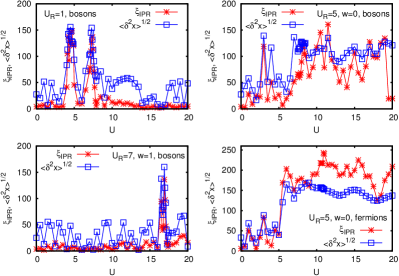
Figure 1: Inverse participation ratio $\xi_{\rm IPR}$ and variance length $\langle\delta^{2}x\rangle^{1/2}=\langle(x-x_{0})^{2}\rangle^{1/2}$ of the time evolution two-particle state for system size $N=512$ and iteration time $t=5120$ (or $t=20480$ for bottom left panel) versus interaction strength $U$. The initial state at $t=0$ is localized either with both particles in the center position $x_{0}=N/2$ (boson case) or antisymmetrized with one-particle in position $x_{0}$ and the other particle in position $x_{0}-1$ (fermion case). Both quantities have been calculated from an effective one-particle density without a center box of size 20% (with respect to system size). The different panels correspond to different cases of interaction range $U_{R}$, decay parameter $w$ and boson/fermion case. Here $\alpha/(2\pi)=(\sqrt{5}-1)/2$ and $\beta=0$.

Fig. 1 shows the dependence of both length scales on the interaction strength $U$ for values up to $U\leq 20$ and different cases of interaction range $U_{R}$ and decay parameter $w$ at iteration time $t=5120$ (or $t=20480$ for the boson case with $U_{R}=7$ and $w=1$). For each case there are a few values of interaction strength where the delocalization is rather strong, even if the weight of the delocalized component is relatively small. For the Hubbard interaction case $U_{R}$ we find the two interesting values $U=4.5$ and $U=7.4$ in a rather good agreement with the results of Ref. flach . However, a closer inspection of the one-particle density reveals that there is still a strong localized main peak close to initial point $x_{0}$ and the delocalization only applies to a small weight of the initial state. We also note that the quantity (9) captures peaks in $U$ in a more clear way compared to (10). We attribute this to additional fluctuations added by a large distance from $x_{0}$ to $x$ values outside of the central box.

The localized main peak can be understood by the assumption that only a small fraction of (two-particle) eigenvectors with specific energy eigenvalues are delocalized while the other eigenvectors remain strongly localized. Indeed, the initial vector $|\psi(0)\!>$, localized at $x_{0}$ and expanded in a basis of two-particle energy eigenstates, contains contributions from all possible energy eigenvalues. The time evolution from the Schrödinger equation only modifies the phases of the energy expansions coefficients but not the amplitudes and therefore the wave packet at arbitrary time $|\psi(t)\!>$ contains rather uniform contributions from the same energy values. Obviously the delocalization effect in the wave packet only happens for the small weight corresponding to the limited fraction of delocalized eigenvectors while the other contributions form the central peak close to the initial position.

We have therefore computed a tail state $|\psi_{\rm tail}(t)\!>$ from the wave packet $|\psi(t)\!>$ by removing (putting to zero) a big 60% center box in a similar way as for $\rho_{\rm eff}(x)$ (but in the two-particle space and using a larger center box). The energy eigenvectors who contribute to $|\psi_{\rm tail}(t)\!>$ obviously only cover the delocalized eigenvectors and assuming that the latter exist only for certain specific energies we can try to determine this energy range (for delocalization) by computing the expectation value $\langle H\rangle$ of $H$ and its energy variance [see Eq. (26)] with respect to $|\psi_{\rm tail}(t)\!>$ (after proper renormalization of $|\psi_{\rm tail}(t)\!>$). Furthermore the square norm $\|\psi_{\rm tail}(t)\|^{2}$, which is the probability of propagating outside the 60% centerbox, gives also a good measure for the delocalization effect.

Table 1: Time evolution parameters for certain cases of short and long range interactions for interaction values with strong delocalization. All rows except the last one correspond to the boson case and the last row to the fermion case. The iteration time is $t=5120$ except for the case with $U=16.9$, $U_{R}=7$ and $w=1$ where $t=20480$. Here $\alpha/(2\pi)=(\sqrt{5}-1)/2$ and $\beta=0$.

$U$	$U_{R}$	$w$	$\xi_{\rm IPR}$	$\langle H\rangle$	$\delta^{2}E$	$\|\psi_{\rm tail}(t)\|^{2^{\phantom{1}}}$
4.4	1	0	129.16	-3.0756	0.2257	0.04175
4.5	1	0	125.22	-3.0645	0.2454	0.0383
4.7	1	0	148.56	-3.0347	0.2594	0.02596
7.2	1	0	109.53	1.8072	0.4891	0.05801
7.4	1	0	136.60	1.1369	3.0897	0.04102
7.8	1	0	15.13	1.8151	0.6851	0.0001974
8.0	5	0	89.26	8.7256	0.3260	0.01406
16.9	7	1	136.06	10.1893	0.5026	0.03268
10.9	5	0	243.17	10.8879	0.4431	0.0795

In Table 1 we show for certain cases with strong delocalization the values of the quantities $\xi_{\rm IPR}$, $\langle H\rangle$, $\delta^{2}E$ and $\|\psi_{\rm tail}(t)\|^{2}$. For $U_{R}=1$ and the first peak at $U\approx 4.5$ the maximum for $\xi_{\rm IPR}$ corresponds to $U=4.7$ while the maximum of $\|\psi_{\rm tail}(t)\|^{2}$ corresponds to $U=4.4$. Therefore the intermediate value $U=4.5$ used in Ref. flach is indeed promising. For all these three values of $U$ the average energy $\langle H\rangle\approx-3.05$ of the tail state corresponds rather well to the approximate eigenvalue region $E\approx-3.1$ at $U=4.5$ for delocalized eigenstates found in flach and confirmed by our detailed eigenvector analysis presented in the next Section. Furthermore, the corresponding energy variance is indeed rather small.

For $U_{R}=1$ there is also a second local maximum of $\xi_{\rm IPR}$ at $U=7.4$ and close to this value there is also a local maximum of $\|\psi_{\rm tail}(t)\|^{2}$ at $U=7.2$. We have also included in Table 1 the value $U=7.8$ which is close to the second interaction value $U=7.9$ used in Ref. flach . The value $U=7.8$ seems less optimal but our eigenvector analysis shows that this value is quite optimal for two different energy ranges $E\approx 1.8$ and $E\approx-2.8$ with well delocalized eigenstates for both energies. According to Table 1 the average energy of the tail state is $\langle H\rangle\approx 1.8$ for $U=7.2$ and $U=7.8$ but with a somewhat larger value of the variance (in comparison to the case $U=4.5$) indicating that the main contributions in the tail state arise from the first energy range $E\approx 1.8$ but the second value $E\approx-2.8$ provides also some smaller contributions therefore increasing the variance. For $U=7.4$ the average energy of the tail state is even reduced to $\langle H\rangle\approx 1.1$ and the variance $\delta^{2}E\approx 3.1$ is quite large which indicates clearly that for this case both energy ranges have more comparable contributions in the tail state. In Fig. 1(a) of Ref. flach these two energy values can be roughly identified with a somewhat stronger delocalization at $E\approx-2.8$. Our eigenvector calculations (see next Section) for larger system sizes confirm that for modest values of system sizes the delocalization is stronger at $E\approx-2.8$ but at larger sizes it is considerable stronger at $E\approx 1.8$.

The values of $\|\psi_{\rm tail}(t)\|^{2}$ between $10^{-4}$ and $5.8\times 10^{-2}$ represent the weight of the delocalized eigenstates in the wave packets. These values are significantly smaller than unity showing that the main contribution still corresponds to the central peak at $x_{0}$ and the localized eigenstates at other energy values but they are also considerably larger than the values $\sim 10^{-14}$ for $U$ values with minimal (or absent) small weight delocalization. In general, the maximal values of $U$ for the two length scales shown in Fig. 1 correspond rather well also to the local maximal values for $\|\psi_{\rm tail}(t)\|^{2}$. For the other three cases of Fig. 1, with long range interaction we can also identify certain values of $U$ with rather strong delocalization (for both length scales and the squared tail norm). According to Table 1 we find for these three cases $\xi_{\rm IPR}\sim 10^{2}$, $\|\psi_{\rm tail}(t)\|^{2}\sim 10^{-2}$ and rather sharp average energy values of the tail state with a small variance.

We have repeated this type of analysis also for many other long range interaction cases and in certain cases we have been able to identify optimal values of $U$ and $E$ for strong delocalization where the approximate energy obtained from the time evolution tail state was used as initial value of $E$ for the Green function Arnoldi method to compute eigenstates (see Sec. 5).

We also computed the inverse participation ratio and the variance length using the full one-particle density of states (including the center box) and also these quantities have somewhat maximal values at the optimum $U$ values for delocalization found above but their maximum values are much smaller than the length scales shown in Fig. 1. Therefore it would be more difficult (or impossible) to distinguish between small weight long range delocalization and high weight small or medium range delocalization (i.e. where the full wave packet delocalizes but for a much smaller length scale). For this reason we prefer to compute the inverse participation ratio and the variance length using the effective one-particle density without center box and with the results shown in Fig. 1.

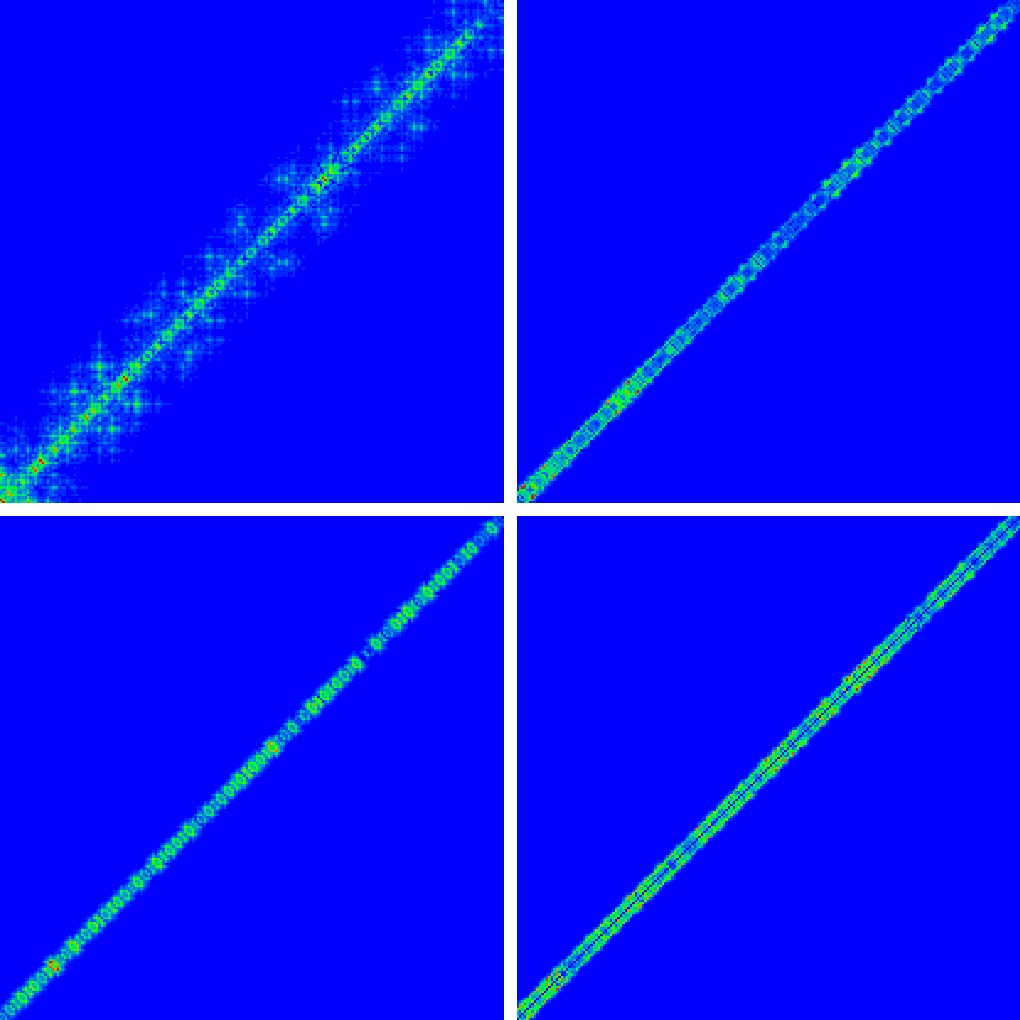
Figure 2: Density plot of time evolution state for $t=5120$ (or $t=20480$ for bottom left panel), system size $N=512$, the four cases of Fig. 1 and with a value of $U$ corresponding to strongest delocalization: $U=4.5$, $U_{R}=1$, boson case (top left panel), $U=8$, $U_{R}=5$, $w=0$, boson case (top right panel), $U=16.9$, $U_{R}=7$, $w=1$, boson case (bottom left panel), $U=10.9$, $U_{R}=5$, $w=0$, fermion case (bottom right panel). We show only zoomed region of size $205\times 205$ with left bottom corner at position $x_{1}=x_{2}=307$ which corresponds to the right/top boundary of the 20% center box. The colors indicate red for maximum, green for medium and blue for minimum values (same distribution of colors in other figures of density plots).

In Fig. 2 we show the density plots of a zoomed region of the time evolution state for the four cases of Fig. 1 and the optimal delocalization values for $U$ ($U=4.5$ for $U_{R}=1$ and the three values given in Table 1 for the cases with $U_{R}>1$ and also mentioned in the figure caption of Fig. 2). The zoomed region correspond to a box of size $205\times 205$ with left bottom corner at position $x_{1}=x_{2}=307$. This value corresponds exactly to the right/top boundary of the 20% center box which has been removed when determining the effective one-particle density of states $\rho_{\rm eff}(x)$. For positions inside the center box between $205$ and $306$ the time evolution state has a strong peaked structure with considerably larger values of the amplitude than the right/top part shown in Fig. 2. The left/lower part (between $0$ and $204$) is similar in structure with similar amplitudes to the right/top part. Fig. 2 clearly confirms the complete small weight delocalization along the diagonal $x_{1}\approx x_{2}$ of the wave packet at sufficiently long iterations times $t=5120$ (or $t=20480$ for the case with $U_{R}=7$ and $w=1$).

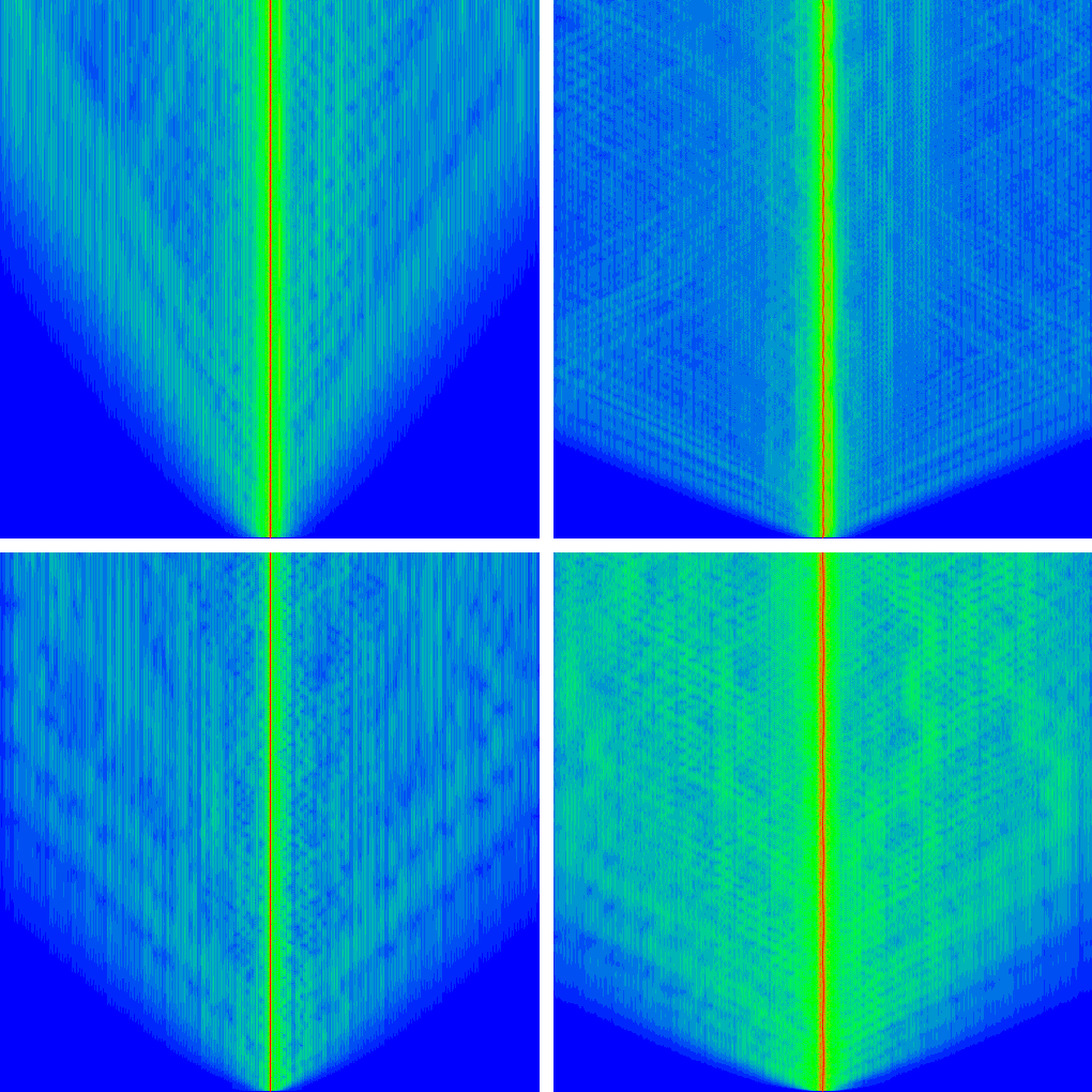
Figure 3: Density plot for the time dependence of one-particle density from the time evolution state with $x$-position ($0\leq x<512$) corresponding to the horizontal axis and time $t$ ($0\leq t\leq 5120$ or $0\leq t\leq 20480$ for bottom left panel) corresponding to the vertical axis. The four panels correspond to the same parameter values of $U$, $U_{R}$, $w$ and boson/fermion cases as in four panels of Fig. 2.

The time evolution of the one-particle density of states can be seen in Fig. 3 with its time dependence corresponding to the vertical axis and position dependence corresponding to the horizontal axis for the same cases and parameters of Fig. 2. In all cases one can identify a strong central peak at $x_{0}$ and a low weight delocalization with a characteristic length scale increasing linearly in time, thus corresponding to a ballistic dynamics already observed for the Hubbard interaction case in flach . One can also observe in Figs. 2 and 3 that for $U=8.0$, $U_{R}=5$, $w=0$, boson case, the weight of the delocalized part of the wave packet is minimal of the four shown cases which is in agreement with the lowest value of $\|\psi_{\rm tail}(t)\|^{2}$ for the same case.

5 Eigenstates for Hubbard interaction

In this Section we present our results for the two-particle eigenstates for the case of the Hubbard interaction with $U_{R}=1$. In order to characterize the delocalization properties of eigenstates we use two quantities. One is the inverse participation ratio in position representation $\xi_{x}$, obtained from the one-particle density of states (8) of eigenstate $|\psi\!>$, by

$$\xi_{x}=\left(\sum_{x}\rho_{\rm 1}^{2}(x)\right)^{-1}\;.$$ (11)

Another one is the inverse participation ratio in energy representation $\xi_{E}$ obtained from an expansion of a two-particle eigenstate $|\psi\!>$ of $H$ in the basis of non-interacting energy product eigenstates $|\phi_{\nu},\phi_{\mu}\!>$ (of $H_{0}$) by

$$\xi_{E}=\left(\sum_{\nu,\mu}\Bigl{|}<\!\phi_{\mu},\phi_{\nu}\,|\,\psi\!>\Bigr{|}^{4}\right)^{-1}.$$ (12)

The quantity $\xi_{x}$ is identical to the “participation number” used in Ref. flach . It is similar (but different) to the quantity (9), used in the previous Section, but for the full one-particle density and not the effective density without the 20% center box. Thus $\xi_{x}$ counts the number of $x$-positions over which the one-particle density extends and obeys the exact inequality $\xi_{x}\leq N$. It is not to be confused with the inverse participation ratio in the two particle $(x_{1},x_{2})$-space, a quantity we did not study. Instead we use the other quantity $\xi_{E}$ that counts the number of non-interacting energy product eigenstates of $H_{0}$ which contribute in the eigenstate. This quantity may be larger than $N$ as we will see for the case of long range interactions in the next Section. It is very convenient to determine $\xi_{E}$ with the second variant of the Green function Arnoldi method where the main computations are done in the energy representation using the non-interacting energy product eigenstates $|\phi_{\nu},\phi_{\mu}\!>$ as basis states. For the case of two particles localized far away from each other, the quantity $\xi_{E}$ is very close to unity while $\xi_{x}$ is closer to $3$-$4$ due to the finite localization length of the one-particle Harper problem. For a ballistic delocalized state along the diagonal $x_{1}=x_{2}$ we expect that both $\xi_{x}$ and $\xi_{E}$ are $\sim CN$ with some constant $C$ of order or a bit smaller than unity.

In this and the next Sections we choose the system size to be a Fibonacci number $N=f_{n}$, the rational case $\alpha/(2\pi)=f_{n-1}/f_{n}$ and $\beta=(\sqrt{5}-1)/2$. However, we have verified that the strong delocalization of eigenstates for certain values of $U$ and $E$ is also valid for the irrational case for arbitrary $N$ with $\alpha/(2\pi)=(\sqrt{5}-1)/2$ and $\beta=0$. For example for $U_{R}=1$, $U=4.5$, $E\approx-3.1$ ($U=7.8$, $E\approx-2.8$) we find for the rational case with $N=4181$ that the eigenstate with maximal $\xi_{E}$ corresponds to $E=-3.09901$, $\xi_{E}=795.960$ and $\xi_{x}=1172.887$ ($E=-2.78600$, $\xi_{E}=501.321$ and $\xi_{x}=475.573$) while for the irrational case with $N=4000$ we have $E=-3.09963$, $\xi_{E}=763.440$ and $\xi_{x}=889.854$ ($E=-2.78716$, $\xi_{E}=559.130$ and $\xi_{x}=588.186$).

We consider as system size $N$ all Fibonacci numbers between 55 and 10946. For each system size we apply the Green function Arnoldi method with a typical Arnoldi dimension $n_{A}\approx 0.7N$-$0.8N$ slightly smaller than $N$ except for the largest case $N=10946$ for which we choose $n_{A}=2000$ or $n_{A}=3000$ and the smallest cases $N=55$ or $N=89$ where we choose $n_{A}\sim 300$-$400$. From all $n_{A}$ Ritz eigenvalues we retain only those with a minimal quality requirement of $\delta^{2}E(\psi)<10^{-8}$ which corresponds roughly to $2/3$ of all $n_{A}$ eigenvalues. It turns out that among these “acceptable” eigenvalues most of them are virtually exact with $\delta^{2}E(\psi)<10^{-20}$ (or even better), especially for the eigenvalues closest to the Green function energy $E$ or with rather large values of $\xi_{E}$ or $\xi_{x}$. Only some eigenvalues at the boundaries $E\pm\Delta E$ (with $\Delta E$ depending on $N$ and $n_{A}$) of the obtained energy band were of modest quality with $\delta^{2}E(\psi)$ between $10^{-20}$ and $10^{-8}$.

Concerning the interaction strength $U$ and the approximate energy range $E$ we present here the detailed results for the eigenvectors of four cases which are $U=4.5$ combined with $E=-3.1$, $U=7.2$ combined with $E=1.8$ and also the less optimal interaction strength $U=7.8$ with two possible energy values $E=-2.8$ and $E=1.8$. For three of theses cases ($U=4.5$, $U=7.2$ and $U=7.8$ with $E=1.8$) the approximate energy range can be obtained as the average energy $\langle H\rangle$ of the tail state computed from the time evolution and given in Table 1. For the last case the second interesting energy value $E=-2.8$ for $U=7.8$ can be found by exact diagonalization for small system sizes ($N=55$ and $N=89$) and was also identified in Fig. 1(a) of Ref. flach . (Actually, the Green function Arnoldi method is for small system sizes also suitable for a full matrix diagonalization by choosing $n_{A}=N(N+1)/2$ identical to the dimension of the symmetrized two-particle Hilbert space.)

The Green function Arnoldi method requires to fix a preferential energy for the Green function which determines the approximate energy range of computed eigenvalues and eigenvectors. For this we use a refinement procedure where at each system size $N$ this energy is either chosen as the eigenvalue of the eigenstate with maximum $\xi_{E}$ obtained from the last smaller system size or, for the smallest system size $N=55$, as one of the above given approximate energy values essentially obtained as the average energy of the time evolution tail state. This systematic refinement is indeed necessary if one does not want to miss the strongest delocalized states since the typical energy width of “good” eigenvalues provided by the method decreases rather strongly with increasing system size, e. g. $\Delta E\sim 10^{-3}$ for $N=10946$.

In this way we obtained indeed the strongest delocalized states up to the largest considered system size. However, for $N=10946$ we added one or two additional runs at some suitable neighbor values for $E$ which allowed us to obtain a more complete set of delocalized states. We also made an additional verification that overlapping states, obtained by two different runs at different $E$ values, were indeed identical for both runs and did not depend on the precise value of $E$ used in the Green function Arnoldi method provided that the eigenvalue of the overlapping eigenstate was sufficiently close to both $E$ values. In general, if one is interested in an eigenstate which by accident is close to the boundary of the good energy interval and is therefore of limited quality, one can easily improve its quality by starting a new run with a Green function energy closer to the eigenvalue of this state.

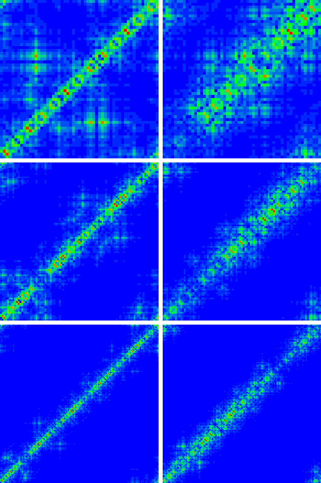
Figure 4: Density plot of FIKS eigenstates with maximal value $\xi_{E}$ for system size $N=55$ (top panels), $N=89$ (center panels), $N=144$ (bottom panels), $U_{R}=1$ and interaction strength $U=4.5$ (left column) or $U=7.8$ (right column). The corresponding energy eigenvalues and values for both types of inverse participation ratios are: Top left: $E=-3.10334$, $\xi_{E}=22.756$, $\xi_{x}=30.794$. Top right: $E=-2.75868$, $\xi_{E}=33.274$, $\xi_{x}=24.901$. Center left: $E=-3.09588$, $\xi_{E}=50.742$, $\xi_{x}=49.867$. Center right: $E=-2.78575$, $\xi_{E}=35.139$, $\xi_{x}=28.198$. Bottom left: $E=3.09966$, $\xi_{E}=61.373$, $\xi_{x}=63.353$. Bottom right: $E=-2.78596$, $\xi_{E}=56.210$, $\xi_{x}=47.958$.

In Fig. 4 we show density plots for the strongest delocalized eigenstates (in $\xi_{E}$) for the two cases $U=4.5$, $E\approx-3.1$ and $U=7.8$, $E\approx-2.8$ and the three smallest system sizes $N=55$, $N=89$ and $N=144$. In all cases the eigenstate extends to the full diagonal along $x_{1}\approx x_{2}$ with a width of about 7 sites ($U=4.5$) or about 15 sites ($U=7.8$) with a quasiperiodic structure of holes or strong peaks. One can also identify some additional peaks with $|x_{1}-x_{2}|\sim 20$-$30$ which can be interpreted as a resonant coupling of the main state with some product state of non-interacting one-particle eigenstates with both particles localized at some modest distance a bit larger than the one-particle localization length $\ell\approx 4.48$ and where the eigenvalue of the main state is very close to the total energy of the product state.

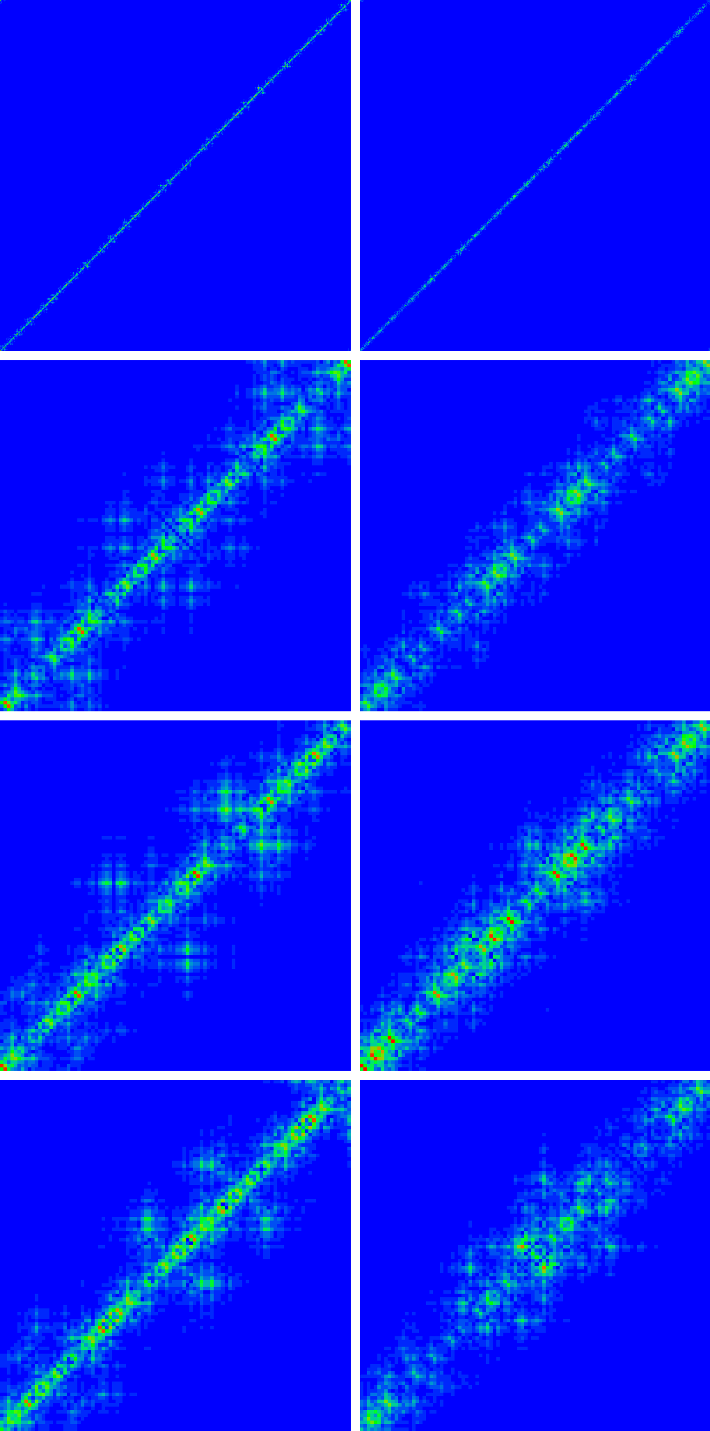
Figure 5: Density plot of FIKS eigenstates with maximal value of $\xi_{E}$ for system size $N=1597$, $U_{R}=1$ (both columns) and interaction strength $U=4.5$, energy eigenvalue $E=-3.09644$, $\xi_{E}=616.638$, $\xi_{x}=716.050$ (left column) or $U=7.8$, $E=-2.78777$, $\xi_{E}=330.269$, $\xi_{x}=355.236$ (right column). The first row corresponds to the full eigenstates and the other rows correspond to zoomed regions of size $100\times 100$ with bottom left corner at position $x_{1}=x_{2}=0$ (second row), $x_{1}=x_{2}=700$ (third row) and $x_{1}=x_{2}=1400$ (fourth row).

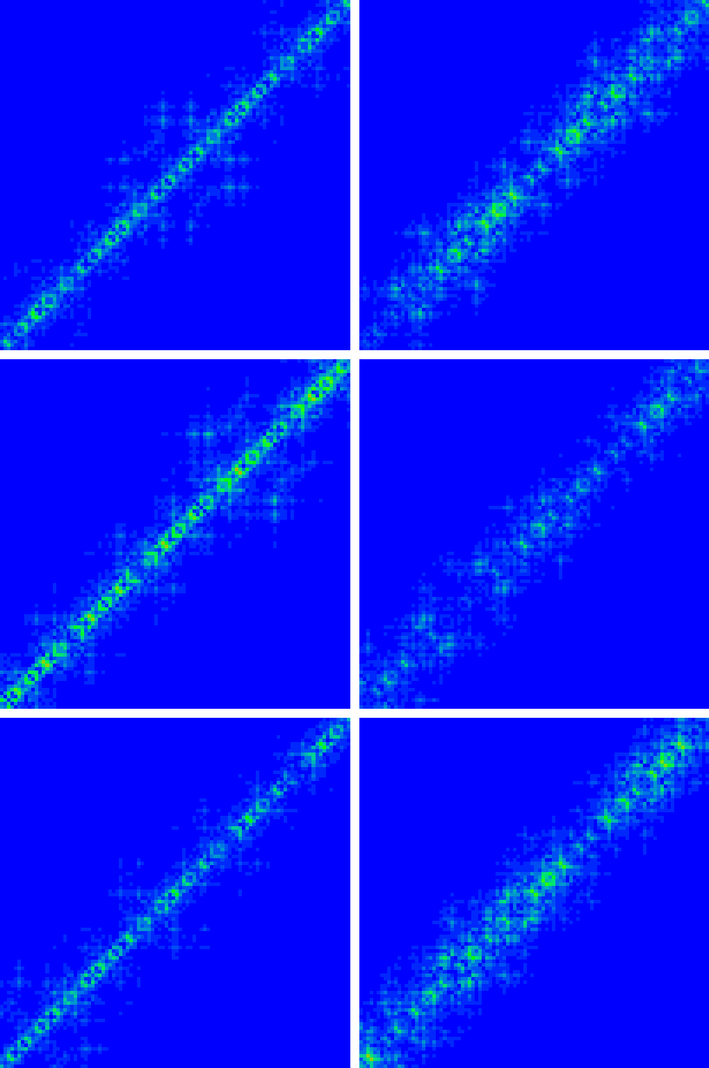
Figure 6: Density plot of FIKS eigenstates with maximal value of $\xi_{E}$ for system size $N=10946$, $U_{R}=1$ (both columns) and interaction strength $U=4.5$, energy eigenvalue $E=-3.09749$, $\xi_{E}=2099.806$, $\xi_{x}=3105.529$ (left column) or $U=7.8$, $E=-2.78707$, $\xi_{E}=952.498$, $\xi_{x}=1147.965$ (right column). All panels correspond to zoomed regions of size $100\times 100$ with bottom left corner at position $x_{1}=x_{2}=0$ (first row), $x_{1}=x_{2}=5000$ (second row) and $x_{1}=x_{2}=10000$ (third row).

In Fig. 5 and Fig. 6, the strongest delocalized states for $N=1597$ ($N=10946$) and the same values of $U$ and approximate energy as in Fig. 4 are shown as full states (only for $N=1597$) and with three zoomed regions of size $100\times 100$ at three different positions on the diagonal (for $N=1597$ and $N=10946$). Again the eigenstates extend to the full diagonal size with a certain width and one can identify a a quasiperiodic structure of holes and peaks and some resonant couplings to product states of non-interacting one-particle eigenstates. Higher quality gif files for the full eigenstate of these (and some other) cases are available for download at webpage .

Figs. 4-6 also show that, apart from the common features, with increasing system size the eigenstates seem to become “thinner”, i. e. the weight of the hole parts seems to increase and the strength of peaks seems to decrease, especially for the case $U=7.8$ and approximate energy $E=-2.8$.

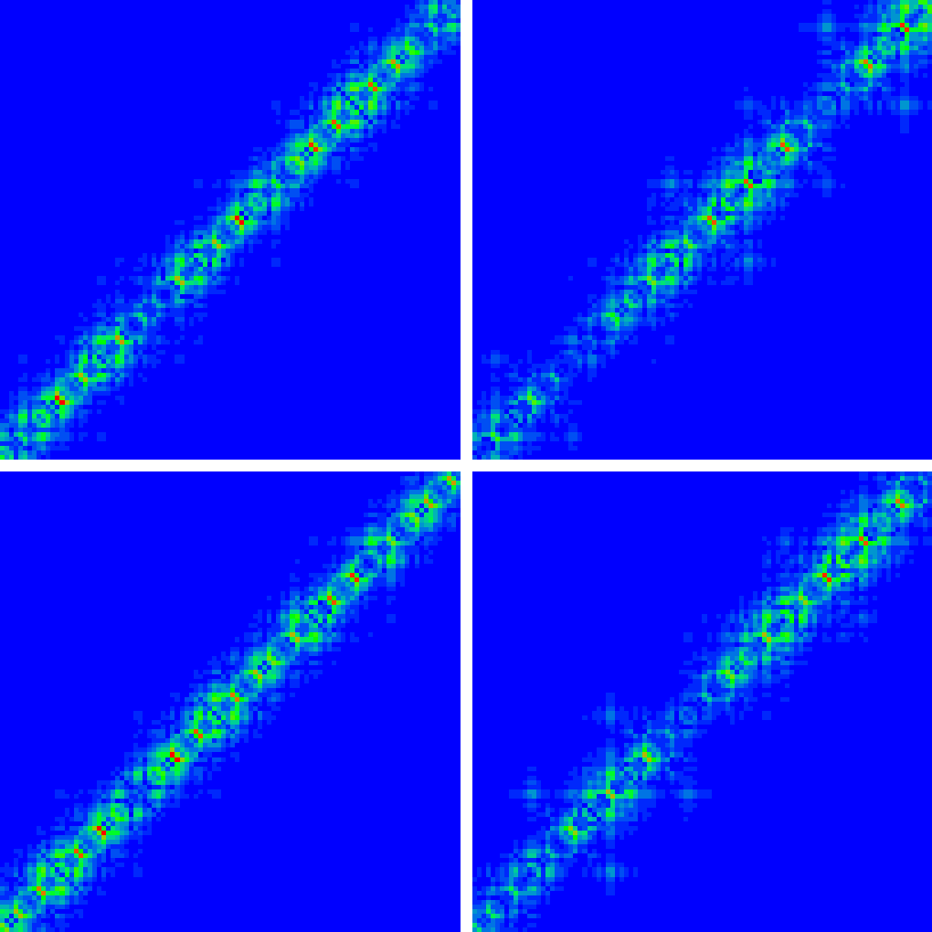
Figure 7: Density plot of FIKS eigenstates with maximal value of $\xi_{E}$ for $E\approx 1.8$, $U_{R}=1$, $U=7.2$ (left column) or $U=7.8$ (right column) and system size $N=1597$ (top panels) or $N=10946$ (bottom panels). All panels correspond to zoomed regions of size $100\times 100$ with bottom left corner at position $x_{1}=x_{2}=700$ (top panels) or $x_{1}=x_{2}=5000$ (bottom panels). The corresponding energy eigenvalues and values for both types of inverse participation ratios are: Top left: $E=1.79597$, $\xi_{E}=638.916$, $\xi_{x}=506.113$, Top right: $E=1.81744$, $\xi_{E}=475.972$, $\xi_{x}=359.239$, Bottom left: $E=1.79652$, $\xi_{E}=5694.610$, $\xi_{x}=4834.890$, Bottom right: $E=1.81741$, $\xi_{E}=2086.088$, $\xi_{x}=1843.227$. The figures obtained for other zoomed regions (on the diagonal) for these states are very similar and these four eigenstates extend clearly to the full diagonal $x_{1}\approx x_{2}$ and all values with $0\leq x_{1}<N$.

Fig. 7 shows a zoomed region of size $100\times 100$ roughly in the middle of the diagonal for strongest delocalized eigenstates for $N=1597$ and $N=10946$ and the two cases $U=7.2$ and $U=7.8$, both with the approximate energy $E=1.8$. Globally one observes in Fig. 7 the same features as in the Figs. 5-6 for the previous two cases but with a detail structure on the diagonal which is significantly different, i. e. quite large width and different pattern for the quasiperiodic peak-hole structure. One observes that the eigenstates for $U=7.2$ are very compact while for $U=7.8$ they are a bit less compact, with more holes, but also with additional small satellite contributions from product pair-states at distance $\approx 20$ from the diagonal. These satellite contributions are absent at $U=7.2$. Apart from this the pattern for both cases in Fig. 7 is rather similar, i.e. the FIKS eigenstates for $E\approx 1.8$, and $U=7.2$ or $U=7.8$ belong to the same family but obviously the value $U=7.2$ is more optimal with a compacter structure, larger values of $\xi_{E}$ and $\xi_{x}$. This is also in agreement with the discussion of the time evolution states in the previous Section. It is interesting to note that even for the case $U=7.8$ with a modest squared tail norm $\approx 2\times 10^{-4}$ (instead of $5\times 10^{-2}$ for $U=7.2$, see Table 1) there are very clear FIKS eigenstates and even at two different energy regions.

We have also calculated eigenstates up to system sizes $N=2584$ for the additional case $U=7.2$ and $E\approx-2.8$ in order to verify if the second energy value is also interesting for $U=7.2$. Here one finds also some FIKS eigenstates but of reduced quality if compared to $U=7.8$ and $E\approx-2.8$, i. e. smaller values of $\xi_{E}$ and $\xi_{x}$ and for larger system sizes the eigenstates do not extend to the full diagonal, i. e. about 20-40% of the diagonal is occupied for $N=2584$. For this additional case we do not present any figures.

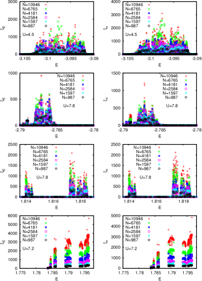
Figure 8: Inverse participation ratio of eigenstates versus eigenvalue energy for the system sizes $N=987$, 1597, 2584, 4181, 6765, 10946 and $U_{R}=1$. The left column of panels correspond to the inverse participation ratio $\xi_{E}$ in energy representation and the right column to the inverse participation ratio $\xi_{x}$ in position representation. First row of panels correspond to $U=4.5$ and the energy region $E\approx-3.098$, second (third) row of panels correspond to $U=7.8$ and $E\approx-2.787$ ($E\approx 1.817$) and fourth row of panels correspond to $U=7.2$ and $E\approx 1.79$.

In Fig. 8 both types of inverse participation ratios $\xi_{E}$ and $\xi_{x}$ of eigenstates are shown as a function of the energy eigenvalue for all four cases (corresponding to Figs. 5-7) with energies in the interesting regions and for the six largest values of the system size between 987 and 10496. Both quantities increase considerably with system size and the overall shape of the cloud of points seems to be similar for each value of $N$ but with a vertical scaling factor increasing with $N$. The figures for $\xi_{E}$ and $\xi_{x}$ are rather similar with somewhat larger (maximum) values for $\xi_{x}$ (except for $U=7.2$ where the maximum value of $\xi_{E}$ is larger). For $U=4.5$ the energy region of delocalized states extends from $E\approx-3.103$ to $E\approx-3.092$ and for $N=10496$ two supplementary runs with Green’s function energy values shifted to the left ($E=-3.104$) and right ($E=-3.094$) from the center ($E=-3.0977$) were necessary to obtain a complete cloud of data points. For $U=7.8$ and approximate energy $E=-2.8$ the main region of delocalized eigenstates extends from $E\approx-2.788$ to $E\approx-2.786$ with a secondary small region at $E\approx-2.789$. For the secondary region and $N=10946$ also an additional run with a shifted Green function energy was necessary. For $U=7.8$ and approximate energy $E=1.8$ the main region of delocalized eigenstates extends from $E\approx 1.8172$ to $E\approx 1.8186$ also with a secondary small region at $E\approx 1.814$ and for this secondary region and $N=10946$ also an additional run with a shifted Green function energy was necessary.

For $U=7.2$ and approximate energy $E=1.8$ the main region of delocalized eigenstates extends from $E\approx 1.793$ to $E\approx 1.797$. For this particular case one observes the absence of eigenstates with very small values of $\xi_{E}\approx 1$ and $\xi_{x}\approx$3-4. We have verified, by choosing different values of the Arnoldi dimension $n_{A}$ and the Green function energy, that the absence of such states is stable with respect to different parameters of the numerical method. Apparently in this energy region there are no strongly localized product states (of one-particle energy eigenstates) with a modest distance between the two particles such that there would be some contribution of them in the initial state used for the Arnoldi method. There may still be other product states in this energy region but with the two particles localized further away such that the Arnoldi method cannot detect them.

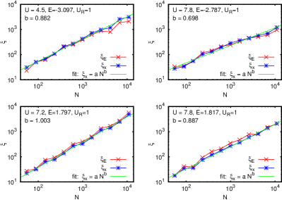
Figure 9: Largest inverse participation ratio (for given values of $N$ and approximate energy) of FIKS eigenstates versus system size $N$ in a double logarithmic scale using all Fibonacci numbers between 55 and 10946. Top (bottom) left panel corresponds to $U=4.5$ ($U=7.2$) and the energy region $E\approx-3.1$ ($E\approx 1.8$). Top (bottom) right panel corresponds to $U=7.8$ and $E\approx-2.8$ ($E\approx 1.8$). The blue line with stars corresponds to the inverse participation ratio $\xi_{x}$ in position representation, the red line with crosses to the inverse participation ratio $\xi_{E}$ in energy representation and the green line to the power law fit $\xi_{x}=a\,N^{b}$ with fit results shown in Table 2. The shown energy values in the panels refer to the eigenvector with maximal $\xi_{E}$ for the largest system size. Note that for given values of $N$ and approximate energy the eigenstates with maximal $\xi_{x}$ and maximal $\xi_{E}$ may be different.

Table 2: Approximate energy $E$ (for largest system size) and results of the power law fit $\xi_{x}=a\,N^{b}$ for the same cases and data sets as in Fig. 9.

$U$	$U_{R}$	$E$	$a$	$b$
$4.5$	$1$	$-3.097$	$0.940\pm 0.137$	$0.882\pm 0.021$
$7.2$	$1$	$1.797$	$0.375\pm 0.054$	$1.003\pm 0.021$
$7.8$	$1$	$-2.787$	$1.878\pm 0.380$	$0.698\pm 0.029$
$7.8$	$1$	$1.817$	$0.559\pm 0.073$	$0.887\pm 0.019$

The scenario of strongly delocalized eigenstates for certain narrow energy bands found in Ref. flach is clearly confirmed also for larger system sizes up to $N=10946$. However, the maximum values of $\xi_{E}$ and $\xi_{x}$ do not scale always linearly with $N$ as can be seen in Fig. 9 which shows the dependence of maximum values of $\xi_{E}$ and $\xi_{N}$ for all four cases (of interaction strength and approximate energy) as a function of the system size $N$ in a double logarithmic scale. Note that in Fig. 9 the data points for maximum $\xi_{E}$ (for given values of $N$, $U$ and approximate energy) may correspond to other eigenstates than for the data points for maximum $\xi_{x}$, i. e. the maximum values for the two quantities are obtained at two different eigenstates. For example for $U=4.5$ and $N=6765$ the eigenstate with maximum $\xi_{E}$ corresponds to $E=-3.09771$, $\xi_{E}=1861.131$, $\xi_{x}=2538.299$ while the eigenstate with maximum $\xi_{x}$ corresponds to $E=-3.09749$, $\xi_{E}=1406.560$, $\xi_{x}=2573.484$, a state which ranks on the 5th position in the list of states with maximum values for $\xi_{E}$. However, despite such particular cases the appearance of large values for $\xi_{E}$ (strong delocalization in one-particle energy representation) or $\xi_{x}$ (strong delocalization in position representation) are rather well correlated which is obvious since the transformation from energy to position representation corresponds somehow to a “smoothing” on the length scale of the one-particle localization length $\ell\approx 4.48$.

The results of the power law fit $\xi_{x}=a\,N^{b}$ using the data sets of Fig. 9 are shown in Table 2. For $U=4.5$ or $U=7.8$ (both energy ranges) the fit values of the exponent $b$, which are either close to $0.9$ or $0.7$, seem to indicate a kind of fractal structure of the eigenstates since even for the largest system sizes the corresponding eigenstates extend to the full length of the diagonal $x_{1}\approx x_{2}$. Therefore the reduction of $\xi_{x}$ with respect to a linear behavior in $N$ is due to the internal structure (appearance of more “holes”). This is also in agreement with our above observation that delocalized eigenstates seem to become thinner for larger systems sizes and this effect is strongest for the case $U=7.8$, $E\approx-2.8$ which also corresponds to the smallest value of the exponent $b=0.698$ among the three cases. However, for $U=7.2$ the exponent is rather precisely unity and no fractal or increasing hole structure (with increasing system size) is visible in the FIKS eigenstates (see also Fig. 7).

6 Eigenstates for long range interaction

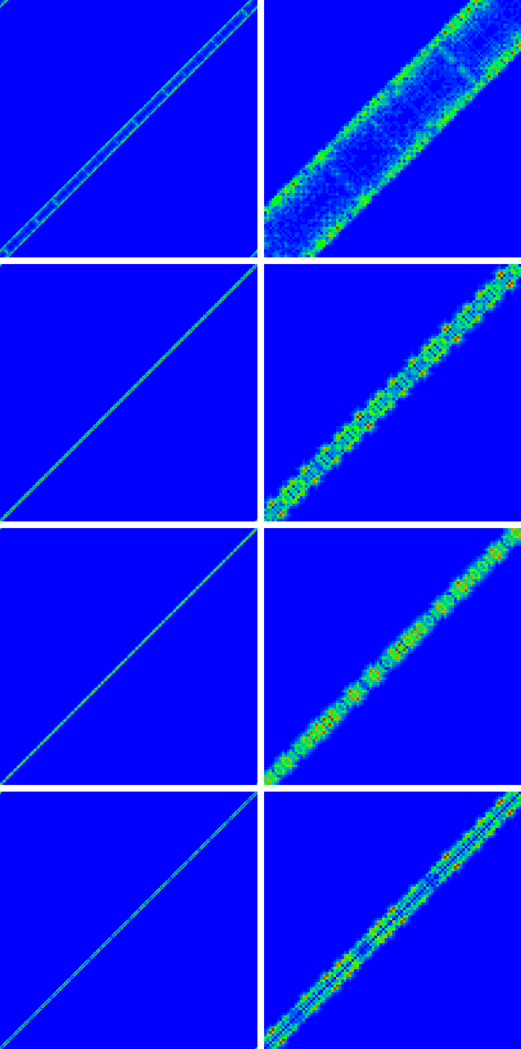
Figure 10: Density plot of FIKS eigenstates for different cases of long range interaction $U_{R}>1$ with maximal inverse participation ratio $\xi_{E}$ in energy representation for $N=610$. The left column corresponds to the full eigenstate and the right column to a zoomed region of size $100\times 100$ with bottom left corner at position $x_{1}=x_{2}=200$. First row: $U_{R}=20$, $w=0$, $U=14$, boson case, energy eigenvalue $E=14.00502$, $\xi_{E}=263.410$, $\xi_{x}=350.519$. Second row: $U_{R}=5$, $w=0$, $U=8$, boson case, $E=8.79607$, $\xi_{E}=787.137$, $\xi_{x}=397.779$. Third row: $U_{R}=7$, $w=1$, $U=17$, boson case, $E=10.22864$, $\xi_{E}=635.918$, $\xi_{x}=307.585$. Fourth row: $U_{R}=5$, $w=0$, $U=10.9$, fermion case, $E=11.53294$, $\xi_{E}=535.618$, $\xi_{x}=360.478$.

We now turn to the case of long range interactions with $U_{R}>1$. We remind that we consider a model where the particles are coupled by the interaction potential $U(x_{1}-x_{2})$ with $U(x)=U/(1+w|x|)$ for $|x|<U_{R}$ U_boundary and $U(x)=0$ if $|x|\geq U_{R}$. For the decay parameter $w$ we mostly choose $w=0$ (i. e. “no decay”) or for the boson case also $w=1$ (decay $\sim|x_{1}-x_{2}|^{-1}$ provided that $|x_{1}-x_{2}|<U_{R}$).

We considered many different cases with $2\leq U_{R}\leq 7$ and one case with $U_{R}=20$ and performed for each case a time evolution analysis as described in Sec. 4 to find good candidates of the interaction strength $U$ for strong delocalization. Using the tail state analysis we also obtained suitable approximate energy values to start the Green function Arnoldi method for the smallest system size $N=55$ we considered. Then we refined the Green function energy for larger system sizes in the same way as described above. In many cases (but not always) this procedure leads to a nice data set of well delocalized two-particle eigenstates for a given narrow energy band. In certain cases the refinement procedure gets trapped at a “wrong” energy, i.e. which is promising for a particular small system size but where the localization saturates at some medium value for $\xi_{E}$ for larger system sizes or is simply less optimal than some other energy. In these cases it might be useful to manually select a different eigenvalue obtained from the last smaller system (e. g. for $N=55$ or $N=89$) to force the refinement of energies into a direction of stronger delocalized states.

We mention that for the larger values of $U_{R}$ the computational cost [$\sim(NU_{R})^{3}$] and the memory requirement [$\sim(NU_{R})^{2}$] of the initial preparation part of the Green function Arnoldi method is considerably increased and therefore we have limited for these cases the maximal considered system size to $N\leq 1597$.

In Fig. 10 we show the strongest delocalized state (in $\xi_{E}$) for $N=610$ and the case $U=14.0$, $U_{R}=20$, $w=0$, boson case (top panels) and the three cases with $U_{R}>1$ already presented in Figs. 1-3 of Sec. 4 (second to fourth row of panels). Concerning the case $U_{R}=7$, $U=16.9$, $w=1$, bosons (of Sec. 4), it turns out that for the eigenstate analysis the interaction strength $U=17.0$ is somewhat more optimal than the case of $U=16.9$. Therefore we show in Fig. 10 (and other figures in this Section) the case of $U=17.0$ instead of $U=16.9$. For each case the left column panel of Fig. 10 shows the full state and the right column panel a zoomed region of size $100\times 100$ with bottom left corner at position $x_{1}=x_{2}=200$ for a better visibility.

The energy eigenvalues of the three boson states in Fig. 10: $E=14.00502$, $E=8.79607$ or $E=10.22864$ (top three rows of panels) correspond quite well to the approximate energies obtained from the tail state analysis of the time evolution wave packet for the same (or very similar) parameters: $\langle H\rangle=14.00247$, $\langle H\rangle=8.72561$ or $\langle H\rangle=10.18926$ (see also Table 1). However for the fermion case (fourth row of panels with $U=10.9$, $U_{R}=5$, $w=0$) the energy eigenvalue of the strongest delocalized state at $N=610$ is $E=11.53294$ while the approximate energy obtained from the tail state analysis $\langle H\rangle=10.88786$ is somewhat different. Here the refinement procedure to optimize $\xi_{E}$ leads already at the first Green function Arnoldi calculation for $N=55$ and $n_{A}=400$ to an energy shift from $10.9$ (as initial Green’s function energy) to $11.5$ (as eigenvalue of the eigenstate with maximum $\xi_{E}$). However, optimizing for $\xi_{x}$ (instead of $\xi_{E}$) or fixing manually the value $E=10.9$ for $N=144$ results in a different set of strongly delocalized eigenstates close to the energy $E=10.84$ with somewhat smaller values for $\xi_{E}$ but larger values for $\xi_{x}$ than the first set of delocalized eigenstates at $E=11.53$.

The eigenstates shown in Fig. 10 have the same common features as the eigenstates shown in Figs. 4-7 for the Hubbard short range interaction discussed previously such as extension to the full diagonal at $x_{1}\approx x_{2}$, a certain width of $\sim 10$-$20$ sites, quasiperiodic structure of holes and peaks etc. but the detail pattern is specific for each case. For the very long interaction range $U_{R}=20$ one observes more a double diagonal structure with main contributions for positions such that $x_{2}\approx x_{1}\pm 20$.

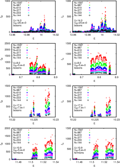
Figure 11: Inverse participation ratio of eigenstates versus eigenvalue energy for the system sizes $N=144$, 233, 377, 610, 987, 1597 and the same four cases with $U_{R}>1$ as in Fig. 10 (see labels in panels for the values of the parameters $U$, $U_{R}$, $w$ and boson or fermion case). The left column of panels correspond to the inverse participation ratio $\xi_{E}$ in energy representation and the right column to the inverse participation ratio $\xi_{x}$ in position representation.

The energy dependence of both $\xi_{E}$ and $\xi_{x}$ for all four cases of Fig. 10 and all system sizes between $144$ and $1597$ is shown in Fig. 11. As in the Hubbard interaction case (see Fig. 8) the typical values of $\xi_{E}$ and $\xi_{x}$ increase systematically with the system size and for each case there is a certain narrow, quite well defined, energy band for strongly delocalized eigenstates.

In addition to this, for the three cases presented in the three lower rows of panels in Fig. 11 one does not see many data points for strongly localized states (with $\xi_{E}\sim 1$) inside or close to this narrow energy band in contrast to Fig. 8 where a lot of eigenstates with very small values of $\xi_{E}$ or $\xi_{x}$ are visible (for three out of four cases). The reason for this is that the total energy for these three cases is outside the interval $|E|<6$ for non-interacting product states (at $\lambda=2.5$) where the two particles are localized more or less far away with only small (or absent) effects due to the interaction. Therefore contributions of such products state cannot be seen for the particular narrow energy bands visible in Fig. 11.

In principle this argument also applies to the first row of panels in Fig. 11 (with $U_{R}=20$ and $U=14.0$), i.e. here products states with particles localized far away cannot be not seen as well. However, for the long interaction range $U_{R}=20$ and due to the fact that the interaction is uniform in this range there are other products states where both particles are localized at a distance smaller than $U_{R}$ which is possible due to the small one-particle localization length $\ell=4.48<20$. The spatial structure of these kind of product states is not modified by the uniform interaction. Therefore they are strongly localized, but obviously the energy eigenvalue of such a short range product range is shifted by the mean value of the uniform interaction $U=14.0$ (with respect to the sum of the two one-particle energies) therefore explaining that it is possible to find such states for energies close to $E\approx 14$. This explains also that more complicated effects of the interaction, such as the creation of strongly delocalized two-particle states, happen if both particles are at an approximate distance $\sim 20$ such that the interaction coupling matrix elements (between non-interacting product states with both particles at critical distance $\sim U_{R}$) have a more complicated and subtle structure due to complicated boundary effects. One may note that this particular type of interaction is similar to the bag model studied in dlstip ; frahm1995 .

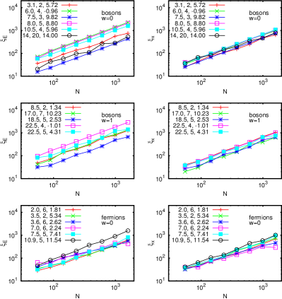
Figure 12: Largest inverse participation ratio (for a given value of $N$) of FIKS eigenstates versus system size $N$ using all Fibonacci numbers between 55 and 1597 for selected cases of long range interactions (same data sets as in Table 3). The left column corresponds to the inverse participation ratio $\xi_{E}$ in energy representation and the right column corresponds to the inverse participation ratio $\xi_{x}$ in position representation. Top (center) panels correspond to the boson case with the decay parameter $w=0$ ($w=1$). Bottom panels correspond to the fermion case with the decay parameter $w=0$. The three numbers in the color labels in the top left corner represent the interaction strength $U$, the interaction range $U_{R}$ and the approximate energy eigenvalue $E$ (for $N=1597$ and the state with largest $\xi_{E}$). Note that for a given value of $N$ and set of interaction parameters the eigenstates with maximal $\xi_{x}$ and maximal $\xi_{E}$ may be different.

Table 3: Approximate energy $E$ and results of the power law fit $\xi_{x}=a\,N^{b}$ for selected cases of long range interactions (same data sets as in Fig. 12). The bottom six rows of the table correspond to the fermion case and the other top rows to the boson case.

$U$	$U_{R}$	$w$	$E$	$a$	$b$
$3.1$	$2$	0	$5.72$	$0.633\pm 0.117$	$0.942\pm 0.032$
$6.0$	$4$	0	$-0.96$	$0.637\pm 0.046$	$0.999\pm 0.013$
$7.5$	$3$	0	$9.82$	$0.465\pm 0.007$	$1.002\pm 0.003$
$8.0$	$5$	0	$8.80$	$0.753\pm 0.055$	$0.978\pm 0.013$
$10.5$	$4$	0	$5.96$	$0.684\pm 0.001$	$1.000\pm 0.000$
$14.0$	$20$	0	$14.00$	$1.118\pm 0.172$	$0.885\pm 0.027$
$8.5$	$2$	1	$1.34$	$0.727\pm 0.062$	$0.986\pm 0.015$
$17.0$	$7$	1	$10.23$	$0.339\pm 0.084$	$1.032\pm 0.043$
$18.5$	$5$	1	$2.53$	$0.485\pm 0.100$	$0.981\pm 0.036$
$22.5$	$4$	1	$-1.01$	$0.635\pm 0.001$	$1.000\pm 0.000$
$22.5$	$5$	1	$4.31$	$0.842\pm 0.168$	$0.936\pm 0.034$
$2.0$	$6$	0	$1.81$	$0.991\pm 0.147$	$0.873\pm 0.026$
$3.5$	$2$	0	$5.34$	$0.696\pm 0.111$	$0.947\pm 0.027$
$3.6$	$6$	0	$2.62$	$1.308\pm 0.158$	$0.807\pm 0.021$
$7.0$	$6$	0	$2.24$	$2.349\pm 0.718$	$0.683\pm 0.053$
$7.5$	$5$	0	$7.41$	$0.793\pm 0.138$	$0.945\pm 0.030$
$10.9$	$5$	0	$11.54$	$0.896\pm 0.141$	$0.949\pm 0.027$

Fig. 12 shows in a double logarithmic scale the size dependence of the maximal inverse participation ratios $\xi_{E}$ (left column) or $\xi_{x}$ (right column) for the above and many other selected cases, with different values of $U$, $U_{R}$, $w$ and boson/fermion case. The typical values of $\xi_{E}$ and $\xi_{x}$ clearly increase strongly with system size $N$ with typical exponents $b\sim 0.7$-$1$ obtained from the power low fit $\xi_{x}=a\,N^{b}$ as can be seen in Table 3. For two particular cases the behavior is even linear with high precision with $b=1$ and a fit error below $0.03$% (the two data sets shown with $b=1.000\pm 0.000$ in Table 3).

Actually, these two cases are also characterized by the absence of strongly localized states with $\xi_{E}\approx 1$ in the narrow energy band (and accessible by the Arnoldi method) in a similar way as the case $U=7.2$ for $U_{R}=1$ discussed previously and one may conjecture that the presence of strongly localized products states (accessible by the Arnoldi method and with a modest distance between both particles) at the same energies as the FIKS eigenstates might be a necessary condition to lower the exponent from the linear behavior $b=1$ to a fractal value $b<1$, eventually due to some weak coupling of FIKS states to strongly localized pairs. Such localized pairs with modest distance would also be reasonable for the appearance of satellite peaks visible in many (but not all) FIKS eigenstates (see discussion in Sec. 5).

For certain other cases of Table 3 the exponents are clearly below 1, e.g. $b\approx 0.7$ or $b\approx 0.8$ indicating a kind of modest fractal structure of the eigenstates in a similar way as for the Hubbard case with $U=7.8$ and $E\approx-2.8$.

Furthermore, both the figure labels of Fig. 12 and also Table 3 provide the approximate energy values for the narrow energy delocalization band and in many cases these energy values also lie inside the interval $|E|<6$ of non-interacting product states with both particles localized far away, confirming that the strong delocalization effect may happen for both cases $|E|<6$ and $|E|>6$.

7 Momentum and energy representation of eigenstates

It is illustrative to present the FIKS eigenstates which are delocalized along the diagonal $x_{1}\approx x_{2}$ in other representations such as a momentum representation using discrete Fourier transform or in the energy representation in terms of non-interacting product one-particle eigenstates, a representation already used for the algorithm of the Green function Arnoldi method described in Sec. 3 and Appendix B.

We first write a two-particle eigenstate with wave function $\psi(x_{1},x_{2})$ for $x_{1},\,x_{2}\in\{0,\,\ldots,\,N-1\}$ in momentum representation by discrete Fourier transform:

$$\bar{\psi}(p_{1},p_{2})=\frac{1}{N}\sum_{x_{1},x_{2}}\,\exp(i\,k_{p_{1}}\,x_{1}+i\,k_{p_{2}}\,x_{2})\,\psi(x_{1},x_{2})$$ (13)

with $k_{p_{j}}=2\pi p_{j}/N$ for $p_{j}=0,\,\ldots,\,N-1$ and $j=1,2$. The momentum eigenfunction (13) can be efficiently evaluated using Fast Fourier Transform using the library fftw3 fftw which also works very well with optimal complexity ${\cal O}(N^{2}\,\log(N))$ (for a two-dimensional discrete Fourier transform) for arbitrary values of $N$, even for prime numbers and not only for powers of two. However, it turns out that the density plot of the momentum eigenfunction (13) has typically a quite complicated or bizarre structure and does not reveal much useful insight in the delocalization effect visible in position representation. Actually, the momentum representation with the simple ordering of momenta $k_{p}$ with $p=0,\,\ldots,\,N-1$ is not appropriate to study the quasiperiodic potential $V_{1}(x)=\lambda\,\cos(\alpha x+\beta)$.

To understand this more clearly let us revisit the eigenvalue equation of an eigenfunction $\phi(x)$ with eigenvalue $\epsilon$ for the one-particle Hamiltonian with this quasiperiodic potential:

$$\epsilon\,\phi(x)=t[\phi(x+1)+\phi(x-1)]+\lambda\cos(\alpha x+\beta)\phi(x)$$ (14)

where we have used a generalized hopping matrix element $t$ and where for simplicity $x$ may take arbitrary integer values for an infinite system and $\alpha/(2\pi)$ is an irrational number such as the golden ratio $\alpha/(2\pi)=(\sqrt{5}-1)/2$. In Ref. aubry a duality transformation was introduced by expanding the eigenfunction in the form:

$$\phi(x)=\sum_{p}\exp[i(\tilde{\beta}x+\alpha p\,x+\beta p)]\,\bar{\phi}(p)$$ (15)

where the sum runs over all integer values of $p$, $\tilde{\beta}$ is some arbitrary parameter and for convenience we have taken out a phase factor $\exp(i\beta p)$ from the precise definition of $\bar{\phi}(p)$. This expansion defines unique coefficients $\bar{\phi}(p)$ only for irrational values of $\alpha$. Inserting (15) into (14) one finds that the function $\bar{\phi}(p)$ obeys a similar eigenvalue equation of the form:

$$\tilde{\epsilon}\,\bar{\phi}(p)=t[\bar{\phi}(p+1)+\bar{\phi}(p-1)]+\tilde{\lambda}\cos(\alpha p+\tilde{\beta})\bar{\phi}(p)$$ (16)

with $\tilde{\epsilon}=2t\epsilon/\lambda$, $\tilde{\lambda}=4t^{2}/\lambda$ and $\tilde{\beta}$ is the parameter used in (15). For $|t|=1$ this transformation maps the case $\lambda>2$ to the case $\tilde{\lambda}=4/\lambda<2$. In Ref. aubry , using this transformation together with Thouless formula (and some technical complications related to a finite size and rational approximation limit of $\alpha$), it was argued that for $\lambda>2$ the eigenfunctions $\phi(x)$ are localized with a localization length $\ell=1/\log(\lambda/2)$ and for the dual case (with $\tilde{\lambda}<2$) the functions $\bar{\phi}(p)$ are delocalized.

The important lesson we can take from the duality transformation (15) is that it uses only a sum over discrete momentum values $q_{p}=(\tilde{\beta}+\alpha\,p){\rm\,mod\,}(2\pi)$, i. e.

$$\phi(x)=\sum_{p}\exp(iq_{p}\,x+i\beta p)\,\bar{\phi}(p),$$ (17)

instead of a continuous integration over $q\in[0,2\pi[$ which would normally be the proper way to perform a Fourier transform from the discrete infinite one-dimensional integer lattice space for $x$ to the continuous variable $q\in[0,2\pi[$. However, the quasiperiodic potential only couples (in the dual equation) momenta $q$ and $\tilde{q}$ such that $\tilde{q}=(q\pm\alpha){\rm\,mod\,}(2\pi)$ and therefore the discrete sum in (15) is sufficient. Furthermore, two momentum values obeying this relation have to be considered as “neighbor” values in dual space, i.e. the natural proper ordering of momentum values is given by the discrete series $q_{p}=(\tilde{\beta}+\alpha\,p){\rm\,mod\,}(2\pi)$ with increasing integer values for $p$.

Let us now consider the case of finite system size $N$ with periodic boundary conditions $\phi(0)=\phi(N)$ in (14). If we want to construct a proper dual transformation for this case we have to chose a rational value for $\alpha/(2\pi)=M/N$ where $0<M<N$ and the integer numbers $M$ and $N$ are relatively prime (if $M$ and $N$ are not relatively prime we would have a periodic potential with a non-trivial period being shorter than the system size requiring an analysis by Bloch theorem etc.). In this case we may directly use (15) to define the duality transformation provided that the sum is limited to the finite set $p=0,\,\ldots,\,N-1$ [and not infinite as for the case of infinite system size with irrational $\alpha/(2\pi)$]. Furthermore, for convenience we chose the parameter $\tilde{\beta}=0$. Then the discrete momentum values $q_{p}$ become

$$q_{p}=(\alpha\,p){\rm\,mod\,}(2\pi)=2\pi\frac{(pM){\rm\,mod\,}N}{N}=k_{\sigma(p)}$$ (18)

where $k_{p}=2\pi p/N$ is the momentum value for the discrete Fourier Transform [see also below (13)] and with $\sigma(p)=(pM){\rm\,mod\,}N$ being a permutation of the set $\{0,\,\ldots,\,N-1\}$ because $M$ and $N$ are relatively prime. We remind that for the eigenstate analysis in the previous Sections we had used the choice $M=f_{n-1}$ and $N=f_{n}$ where $f_{n}$ is the $n$-th Fibonacci number and we note that two subsequent Fibonacci numbers are indeed always relatively prime. For this particular choice we call the permutation $\sigma(p)$ the golden permutation. The permutation property of $\sigma(p)$ and Eq. (18) ensure that the discrete momentum values $q_{p}$ of the dual transformation (15) coincide exactly with the discrete momentum values used for the discrete Fourier Transform for a finite lattice of size $N$. However, there is a modified ordering between $q_{p}$ and $k_{p}$ because of the permutation and “neighbor” momenta $k_{p}$ and $k_{p+1}$ of the discrete Fourier Transform are not neighbor values for the dual transformation and therefore the direct naive momentum representation (13) is not appropriate. The proper dual transformed representation corresponds to the golden permutation Fourier representation defined by

$$\bar{\psi}_{g}(p_{1},p_{2}) = \bar{\psi}(\sigma(p_{1}),\sigma(p_{2}))$$

$$= \sum_{x_{1},x_{2}}\,\exp(i\,q_{p_{1}}\,x_{1}+i\,q_{p_{2}}\,x_{2})\,\psi(x_{1},x_{2})$$

where the second identity with $q_{p}$ (instead of $k_{p}$) is valid due to (18). For $\bar{\psi}_{g}(p_{1},p_{2})$ neighbor values in $p_{1}$ or $p_{2}$ correspond indeed to neighbor values in the dual transformation.

We mention that for a finite system size $N$ and an irrational choice of $\alpha/(2\pi)$ the momenta, $q_{p}=(\alpha\,p){\rm\,mod\,}(2\pi)$, used for the duality transformation do not coincide exactly with the discrete momenta of the discrete Fourier transform, in particular the quantity

$$\sigma(p)=\left(\frac{Np\alpha}{2\pi}\right){\rm\,mod\,}N$$ (20)

would typically not be an integer number. At best one could try to define an approximate duality transformation with a modified permutation by rounding (20) to the next integer number but even in this case one would typically not obtain a permutation and it would be necessary to correct or modify certain $\sigma(p)$ values in order to avoid identical $\sigma(p)$ values for different integers $p$.

If we want to choose a finite system size $N$ which is not a Fibonacci number we could try for the choice of $\alpha/(2\pi)$ a rational approximation $M/N$ of the golden ratio $(\sqrt{5}-1)/2$ with $M$ being the closest integer to $N(\sqrt{5}-1)/2$ and the denominator fixed by the given system size. However, in this case one might obtain a value of $M$ such that $M$ and $N$ are not relatively prime and (if we want to keep the same denominator) it would necessary to chose a different value of $M$ relatively prime to $N$ and still rather close to $N(\sqrt{5}-1)/2$ therefore reducing the quality of the rational approximation. For this reason we have in the preceding Sections mostly concentrated on the choice of Fibonacci numbers for the system size such that we can use the best rational approximation for the golden number and where we can always define in a simple and clear way the golden permutation by $\sigma(p)=(pf_{n-1}){\rm\,mod\,}f_{n}$.

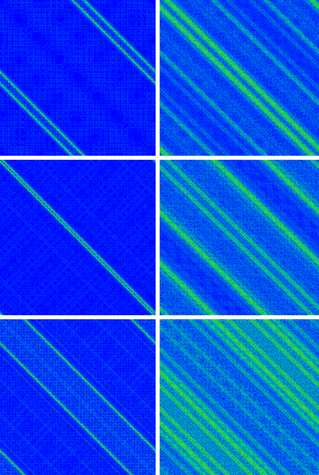
Figure 13: Density plot of the three FIKS eigenstates in golden permutation Fourier representation with largest values of $\xi_{E}$ for $N=610$, $U_{R}=1$, $U=4.5$ (left column) or $U=7.8$ (right column). The corresponding energy eigenvalues and values for both types of inverse participation ratios are: Top left: $E=-3.09750$, $\xi_{E}=249.137$, $\xi_{x}=271.208$. Top right: $E=-2.78586$, $\xi_{E}=211.058$, $\xi_{x}=194.241$. Center left: $E=-3.09964$, $\xi_{E}=239.312$, $\xi_{x}=265.885$. Center right: $E=-2.78599$, $\xi_{E}=200.958$, $\xi_{x}=176.454$. Bottom left: $E=-3.09815$, $\xi_{E}=233.773$, $\xi_{x}=250.700$. Bottom right: $E=-2.78593$, $\xi_{E}=190.171$, $\xi_{x}=193.885$.

In Fig. 13 the three eigenstates with maximum $\xi_{E}$ for $N=610$, $U_{R}=1$ and the two cases $U=4.5$ and $U=7.8$ (and $E\approx-2.8$) are shown in the golden permutation Fourier representation. One sees clearly that for the center of mass coordinate there is a strong momentum localization around a few typical values while for the relative coordinate all momentum values seem to contribute to the eigenstate leading to momentum delocalization in this direction. This is just dual to the typical behavior of such eigenstates in position representation with delocalization in the center of mass coordinate and localization in the relative coordinate. However, the precise detailed structure, in momentum space on a length scale of a few pixels and well inside the stripes seen in Fig. 13, is still quite complicated and subtle.

The “localization length” in momentum space for the center of mass coordinate is considerably shorter for the case $U=4.5E$ with about 10 pixels (i. e. discrete momentum values) than for the other case $U=7.8$ (and $E\approx-2.8$) with about 30 pixels. This observation relates to the stronger quasiperiodic hole-peak structure in the eigenstates seen in Figs. 4-6 for the case $U=7.8$ (and $E\approx-2.8$).

We have also tried for the irrational case and non-Fibonacci numbers for $N$ to define an approximate golden permutation which in principle provides similar figures as in Fig. 13 but with a considerable amount of additional irregularities concerning the momentum structure etc.

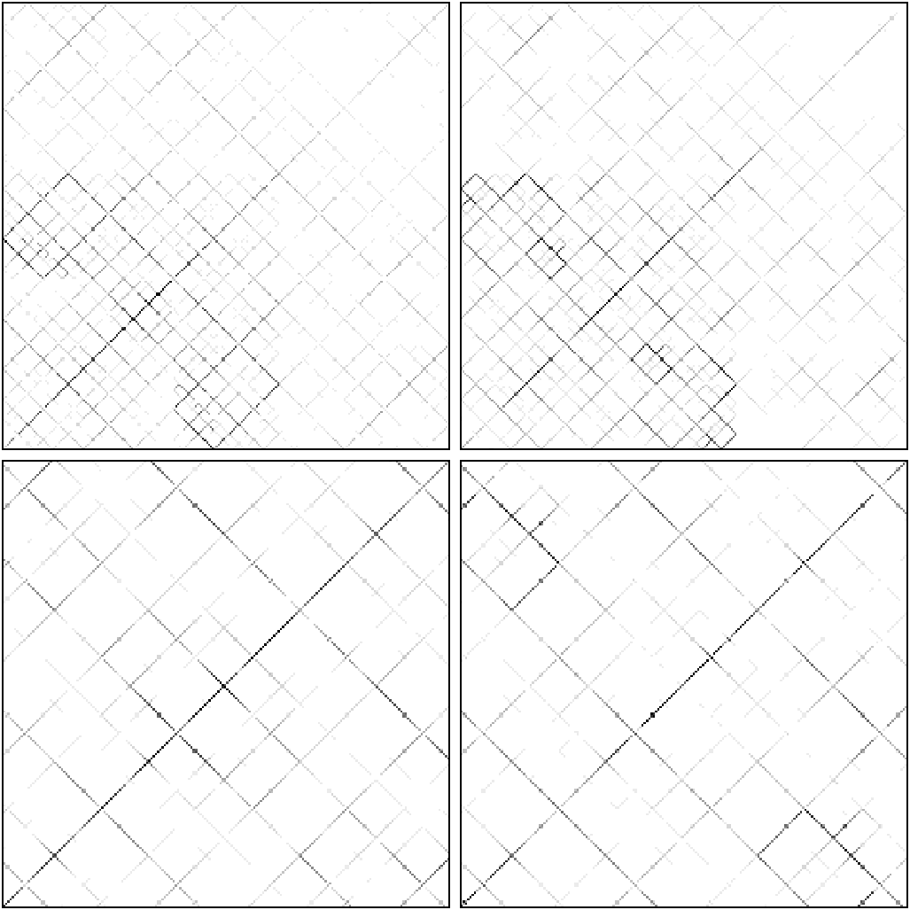
Figure 14: Density plot of the FIKS eigenstates in non-interacting energy representation with the largest value of $\xi_{E}$ for $N=233$ (top panels) or $N=610$ (bottom panels), $U_{R}=1$, $U=4.5$ (left column) or $U=7.8$ (right column). Black represents maximum, grey medium and white minimum values of the expansion amplitudes of the shown eigenstate with respect to non-interacting energy product eigenstates $|\phi_{\nu},\phi_{\mu}\!>$. The horizontal (vertical) axis corresponds to the index $\nu$ ($\mu$) ordered with respect to increasing values of the corresponding one-particle energy $\epsilon_{\nu}$ ($\epsilon_{\mu}$) of the first (second) particle. Top panels for $N=233$ correspond to full eigenstates and bottom panels for $N=610$ correspond to a zoomed region of size $200\times 200$ with left bottom corner at position $x_{1}=x_{2}=100$. The corresponding energy eigenvalues and values for both types of inverse participation ratios are: Top left: $E=-3.09669$, $\xi_{E}=107.409$, $\xi_{x}=106.818$. Top right: $E=-2.78569$, $\xi_{E}=117.697$, $\xi_{x}=102.577$. Bottom left: $E=-3.09750$, $\xi_{E}=249.137$, $\xi_{x}=271.208$. Bottom right: $E=-2.78586$, $\xi_{E}=211.058$, $\xi_{x}=194.241$.

Another type of interesting eigenvector representation is obtained by an expansion of a two-particle eigenstate in the basis $|\phi_{\nu},\phi_{\mu}\!>$ of non-interacting one-particle product eigenstates. Fig. 14 shows black and white density plots for the amplitudes of certain eigenstates in such a representation for the two sizes $N=233$ and $N=610$ and the two values of the interaction $U=4.5$ and $U=7.8$ (both for $U_{R}=1$). Both axis correspond to the one-particle index ordered with respect to increasing values of the corresponding one-particle energy. We remind that in the second variant of the Green function Arnoldi method the main calculations are actually done in this energy representation, which is therefore more easily accessible than the standard position representation.

One observes a kind of self-similar structure with (approximate) golden ratio rectangles of different sizes along the diagonals. The inverse participation ratio $\xi_{E}$ in energy representation corresponds approximately to the number of black dots in the black and white density plots of Fig. 14.

We mention that when the one-particle eigenstate ordering in the energy representation is done with respect to the maximum positions of the one-particle eigenstates (instead of the one-particle energy) one obtains a clear banded structure with main values/peaks for $\nu\approx\mu\pm 5$ (Figure not shown).

8 Implications for cold atom experiments

Motivated by recent experiments on cold atoms bloch we present also some results for a modified value of the flux parameter $\alpha$ used in the quasiperiodic potential $V_{1}(x)$. In the experiment of Ref. bloch the rational value for $\alpha/(2\pi)\approx 532/738=266/369$ was used. This value has the finite continued fraction expansion $[0;1,2,1,1,2,1,1,8]$ with

$$[a_{0};a_{1},a_{2},a_{3},\ldots]=a_{0}+\cfrac{1}{a_{1}+\cfrac{1}{a_{2}+\cfrac{1}{a_{3}+\cdots}}}.$$ (21)

We define two numbers $\alpha_{j}$, $j=1,2$ such that $\alpha_{j}/(2\pi)$ is irrational and close to the experimental rational value by

$$\frac{\alpha_{1}}{2\pi}=[0;1,2,1,\ldots]=\frac{\sqrt{10}-1}{3}=0.7207592200561264\ldots$$ (22)

and

$$\frac{\alpha_{2}}{2\pi} = [0;1,2,1,1,2,1,1,8,\ldots]$$

$$= \frac{\sqrt{39999}-169}{43}=0.7208720926598791\ldots$$

where the initial pattern of shown coefficients in the continued fraction expansion (except the leading zero) repeats indefinitely with a period of 3 (or 8) for the case of $\alpha_{1}$ (or $\alpha_{2}$). The first choice provides a “stronger” irrational number for $\alpha_{1}/(2\pi)$ while the second choice is closer to the experimental value. In this Section we choose for all numerical computations one of these two values (or rational approximations of them for the eigenvector calculations) and furthermore we fix the phase offset and the interaction range by $\beta=(\sqrt{5}-1)/2$ and $U_{R}=1$.

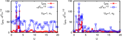
Figure 15: Inverse participation ratio $\xi_{\rm IPR}$ and variance length $\langle\delta^{2}x\rangle^{1/2}=\langle(x-x_{0})^{2}\rangle^{1/2}$ of the time evolution two-particle state for system size $N=512$, iteration time $t=5120$ and $\alpha_{1}$ (left panel) or $\alpha_{2}$ (right panel) versus interaction strength $U$. The initial state at $t=0$ is localized with both particles in the center position $x_{0}=N/2$. Inverse participation ratio and variance length have been calculated from an effective one-particle density without a center box of size 20% (with respect to system size). The data points for $2<U<2.5$ have been calculated with a doubled iteration time $t=10240$. The values of $\alpha_{1},\alpha_{2}$ from (22), (8) correspond to experimental conditions of bloch .

First, we performed the time-evolution analysis already described in Sec. 4 using either $\alpha_{1}$ or $\alpha_{2}$. Fig. 15 shows the dependence of the inverse participation ratio $\xi_{\rm IPR}$ and the variance length [both computed without the 20% center box, see (9) and (10)] on the interaction strength $U$ ($0\leq U\leq 20$) for a system size $N=512$ and an iteration time $t=5120$. As in Sec. 4 we chose for $t=0$ an initial state with both particles localized at the center point $x_{0}=N/2$. For both $\alpha$ values we observe strong peaks for both length scales at values $U=2.25$-$2.3$ and $U=3.6$ indicating the possible existence of FIKS states at these interaction values (or very close). A closer inspection reveals that the first peak close to $U=2.25$ requires a longer iteration time $t=10240$ in order to provide saturation of the two length scales and therefore in Fig. 15 the data points for $2<U<2.5$ are computed with this increased iteration time.

Table 4: Time evolution parameters for the interaction values $U=2.25$ and $U=3.6$ and both values of $\alpha$ using the data sets of Fig. 15. These interaction values correspond to the local maxima of the squared tail norm $\|\psi_{\rm tail}(t)\|^{2}$. Note that for $U$ close to $2.25$ the local maxima visible in Fig. 15 of the length scale $\xi_{\rm IPR}$ (computed without the 20% center box) correspond actually to $U=2.3$ with slightly larger values than for $U=2.25$.

$\alpha$	$U$	$t$	$\xi_{\rm IPR}$	$\langle H\rangle$	$\delta^{2}E$	$\|\psi_{\rm tail}(t)\|^{2^{\phantom{1}}}$
$\alpha_{1}$	2.25	5120	32.27	-4.744	0.475	0.00884
$\alpha_{1}$	2.25	10240	79.48	-4.828	0.127	0.107
$\alpha_{1}$	3.6	5120	101.12	-0.893	0.159	0.0449
$\alpha_{2}$	2.25	5120	30.18	-4.717	0.587	0.00562
$\alpha_{2}$	2.25	10240	64.58	-4.826	0.140	0.0709
$\alpha_{2}$	3.6	5120	45.45	-0.878	0.215	0.0188

Table 4 summarizes the results of the quantities $\xi_{\rm IPR}$, $\langle H\rangle$, $\delta^{2}E$ and $\|\psi_{\rm tail}(t)\|^{2}$ (see Sec. 4 for the precise definition of them) at the two peak values $U=2.25$ and $U=3.6$. The values of $\xi_{\rm IPR}$ in Table 4 for $U=2.25$ and $t=10240$ do actually not exactly correspond to the first local maximum visible in Fig. 15 because $\xi_{\rm IPR}$ is maximal at $U=2.3$ while the value of $U=2.25$ corresponds to the local maximum of $\|\psi_{\rm tail}(t)\|^{2}$. However, detailed eigenvector calculation for these two interaction values confirm that globally the value $U=2.25$ is slightly more optimal than $U=2.3$ with stronger delocalization.

In Table 4 we provide for the case $U=2.25$ also the results for the two iteration times $t=5120$ and $t=10240$. Obviously, $\xi_{\rm IPR}$ and $\|\psi_{\rm tail}(t)\|^{2}$ are considerably increased at $t=10240$ but already at $t=5120$ the strong delocalization FIKS effect is visible. The average energy value of the tail state is rather sharp with a modest variance $\delta^{2}E$ for all cases, but also with an additional significant decrease of $\delta^{2}E$ between $t=5120$ and $t=10240$ (for $U=2.25$).

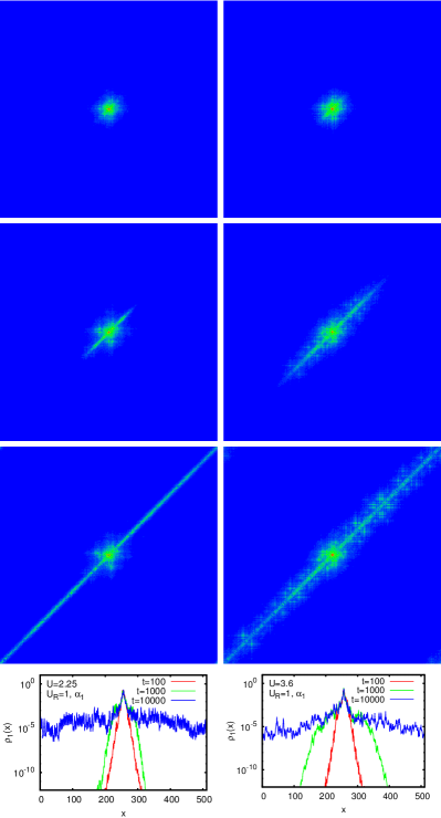
Figure 16: Density plot (three top rows of panels) of time evolution two-particle states for system size $N=512$, the case $\alpha_{1}$, interaction range $U_{R}=1$, interaction strength $U=2.25$ (left column) or $U=3.6$ (right column), iteration times $t=100$ (first row), $t=1000$ (second row) and $t=10000$ (third row); panels show the whole system range $(0\leq x_{,}x_{2}<512)$. The fourth row of panels shows the one-particle density $\rho_{1}(x)$ in a semi-logarithmic representation for the same states as in the three top rows of panels. The initial state at $t=0$ is localized with both particles in the center position $x_{0}=N/2$.

Globally Fig. 15 and Table 4 show that the FIKS effect is stronger for $U=2.25$ but at this value it requires a longer iteration time to be clearly visible. This observation is also confirmed by Fig. 16 which shows for $\alpha_{1}$ and both interaction values $U=2.25$ and $U=3.6$ the density plots and the one-particle density of three time evolution states at $t=100$, $t=1000$ and $t=10000$. In both cases the state is clearly localized at the beginning at $t=100$ and it is delocalized over the full system size at $t=10000$ (with a small weight and along the diagonal $x_{1}\approx x_{2}$ as discussed in Sec. 4). However, for the intermediate time $t=1000$ the state for $U=2.25$ is considerably less delocalized than the state for $U=3.6$ at the same iteration time clearly confirming the slower delocalization speed for $U=2.25$. Thus the velocity of FIKS pairs is smaller at $U=2.25$ than at $U=3.6$ but the weight of FIKS pairs in the initial state is larger at $U=2.25$. Apart from this the delocalized tails of the state at $t=10000$ appear somewhat “stronger” or “thicker” for $U=2.25$ explaining the larger values of $\xi_{\rm IPR}$ (for $\alpha_{1}$). Note that Fig. 16 shows the full time evolution states while Fig. 2 in Sec. 4, with the golden ratio value for $\alpha/(2\pi$), shows only a zoomed range for the right delocalized branche between the right border of the 20% center box and the right border of the full system.

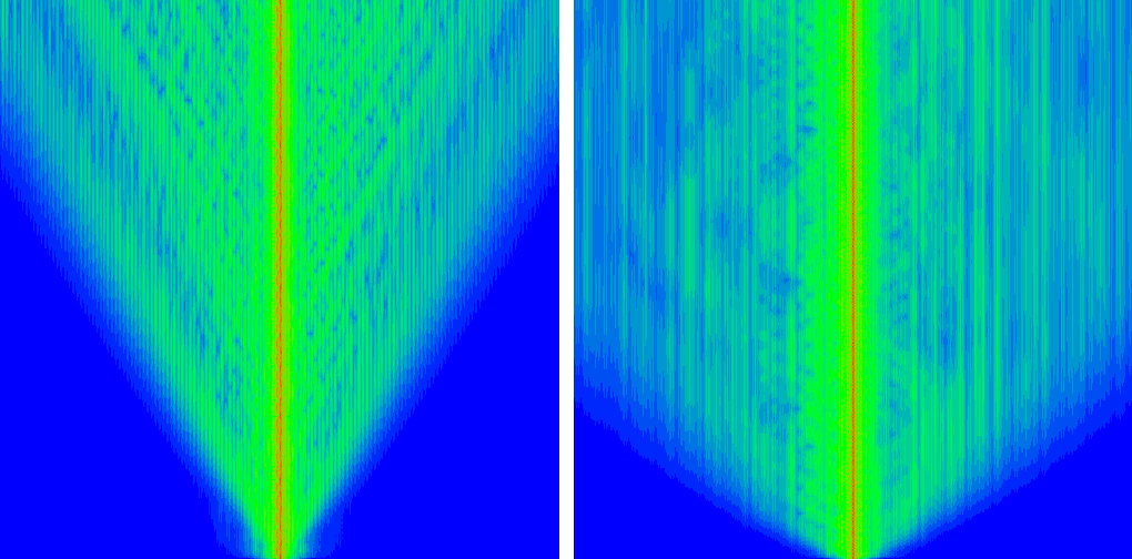
Figure 17: Density plot for the time dependence of one-particle density from the time evolution state with $x$-position ($0\leq x<512$) corresponding to the horizontal axis and time $t$ ($0\leq t\leq 10240$) corresponding to the vertical axis. Here $U=2.25$ (left panel), $U=3.6$ (right panel) and $\alpha=\alpha_{1}$, $U_{R}=1$.

Fig. 17 shows the time evolution of the one-particle density (for $\alpha_{1}$) with the $x$-dependence corresponding to the horizontal axis and with the $t$-dependence ($0\leq t\leq 10240$) corresponding to the vertical axis. This figure provides clear and additional confirmation that the delocalization effect is stronger and slower for $U=2.25$ than for $U=3.6$. It also confirms the linear (ballistic) increase of the delocalized part of the state with time (see also Fig. 3). We mention that the other value $\alpha_{2}$ provides very similar figures as Figs. 15 and 16 with a slightly reduced delocalization effect for both interaction values.

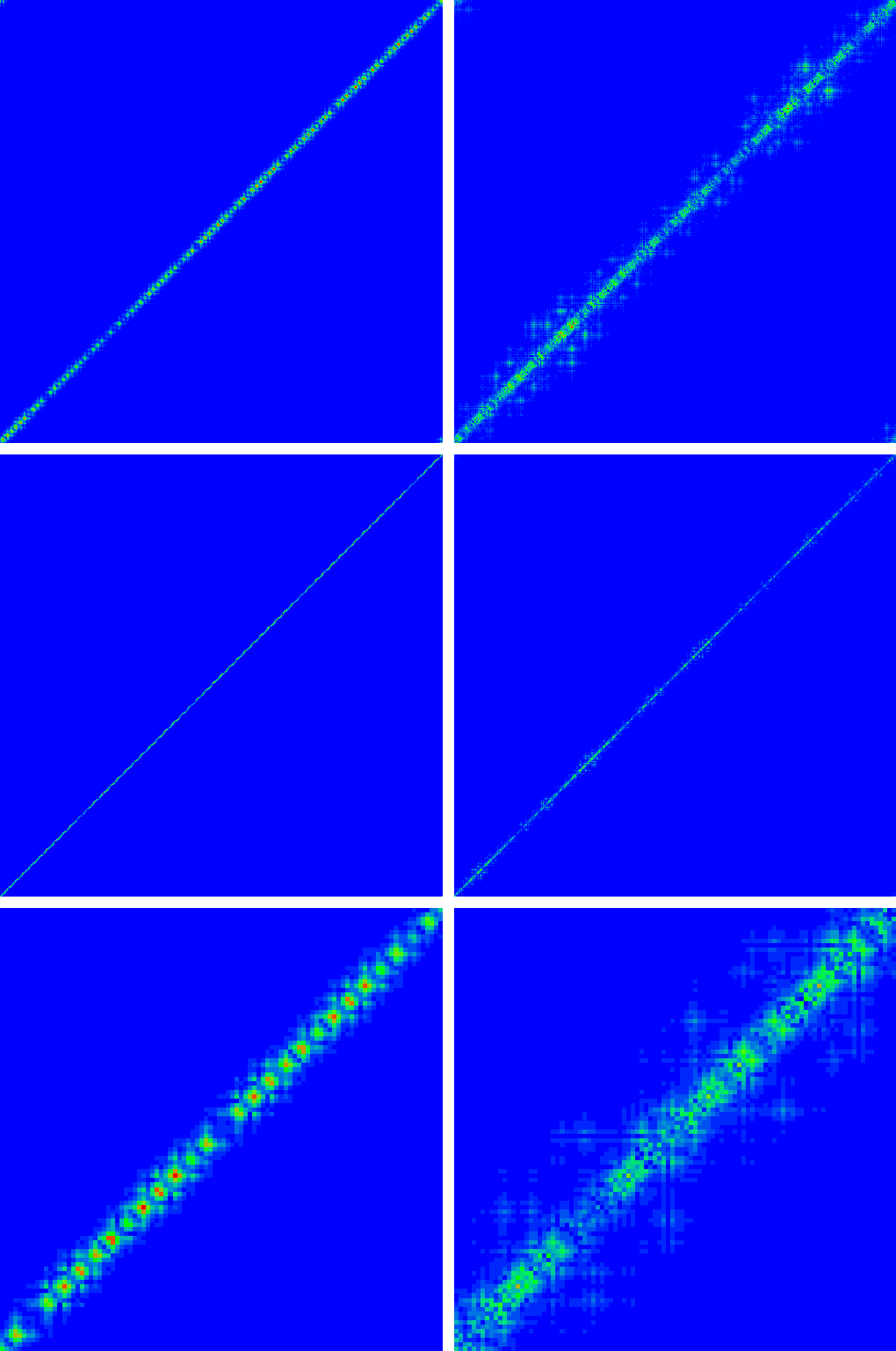
Figure 18: Density plot of FIKS eigenstates for rational approximations of $\alpha_{2}/(2\pi)$ and $U=2.25$ (left column), $U=3.6$ (right column), $N=369$ (top panels), $N=1605$ (center and bottom panels); $U_{R}=1$. The corresponding energy eigenvalues and values for both types of inverse participation ratios are: Top left: $E=-4.85051$, $\xi_{E}=98.462$, $\xi_{x}=118.308$. Top right: $E=-0.92196$, $\xi_{E}=113.232$, $\xi_{x}=108.389$. Center left: $E=-4.84994$, $\xi_{E}=428.375$, $\xi_{x}=566.237$. Center right: $E=-0.92198$, $\xi_{E}=309.040$, $\xi_{x}=260.125$. Bottom panels show a zoomed region of size $100\times 100$ with left bottom corner at position $x_{1}=x_{2}=350$ of the center panels.

Following the procedure described in the beginning of Sec. 5 we have also computed eigenstates using the Arnoldi Green function method with the average energy values $\langle H\rangle$ of Table 4 as initial Green’s function energy for the smallest system size. The Green function energies are refined for larger system sizes using the energy eigenvalue of a well delocalized eigenstate of the last smaller system size. Following the spirit of the previous explications [see text between Eqs. (17) and (18)] we choose rational approximations of $\alpha_{1}/(2\pi)$ and $\alpha_{2}/(2\pi)$ using their continued fraction expansions (22) and (8) which provide suitable system sizes given as the denomators of the rational approximations. Using a minimal (maximal) system system size $\sim 40$ ($\sim 10000$) this provides for $\alpha_{1}$ the values $N=43$, 111, 154, 265, 684, 949, 1633, 4215, 5848, 10063 and for $\alpha_{2}$ the values $N=43$, 369, 412, 1193, 1605, 2798, 7201, 9999. Note that the system size $369$ corresponds to the rational approximation $\alpha_{2}/(2\pi)\approx 266/369$ used in the experiments of Ref. bloch . For each system size we use the corresponding rational approximation of $\alpha_{j}/(2\pi)$ ($j=1,\,2$) and $\beta=(\sqrt{5}-1)/2)$ to determine numerically certain eigenstates by the Green function Arnoldi method.

In Fig. 18 we show selected strongly delocalized eigenstates for $\alpha_{2}$ and the two interaction values $U=2.25$ and $U=3.6$ and the system sizes $N=369$ and $N=1605$. All eigenstates provide nice FIKS pairs with a quite specific particular pattern on the diagonal $x_{1}\approx x_{2}$ which correponds, for each of the two interaction values, rather well to the pattern of (the delocalized tails of) the time evolution states for $t=10000$ visible in Fig. 16. For $N=1605$ the pattern for $U=2.25$ seems be to considerably more compact than the pattern for $U=3.6$ which is also confirmed by a considerably larger value of $\xi_{x}$. The eigenstates for the $\alpha_{1}$ case are very similar for comparable system sizes.

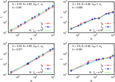
Figure 19: Largest inverse participation ratio (for given values of $N$ and approximate energy) of FIKS eigenstates versus system size $N$ in a double logarithmic scale for $U_{R}=1$, for rational approximations of $\alpha_{1}/(2\pi)$ (top panels) or $\alpha_{2}/(2\pi)$ (bottom panels) and for $U=2.25$, $E\approx-4.85$ (left column) or $U=3.36$, $E\approx-0.92$ (right column). The used system sizes are 43, 111, 154, 265, 684, 949, 1633, 4215, 5848, 10063 given by the denominators of the rational approximations of $\alpha_{1}/(2\pi)$ and 43, 369, 412, 1193, 1605, 2798, 7201, 9999 for the rational approximations for $\alpha_{2}/(2\pi)$. The blue line with stars corresponds to the inverse participation ratio $\xi_{x}$ in position representation, the red line with crosses to the inverse participation ratio $\xi_{E}$ in energy representation and the green line to the power law fit $\xi_{x}=a\,N^{b}$ with fit values given in Table 5. Note that for given values of $N$ and approximate energy the eigenstates with maximal $\xi_{x}$ and maximal $\xi_{E}$ may be different.

Table 5: Results of the power law fit $\xi_{x}=a\,N^{b}$ for the four cases of Fig. 19.

$U$	$U_{R}$	$\alpha$	$E$	$a$	$b$
$2.25$	$1$	$\alpha_{1}$	$-4.85$	$0.424\pm 0.013$	$0.990\pm 0.004$
$3.6$	$1$	$\alpha_{1}$	$-0.92$	$1.878\pm 0.348$	$0.685\pm 0.027$
$2.25$	$1$	$\alpha_{2}$	$-4.85$	$0.418\pm 0.055$	$0.971\pm 0.018$
$3.6$	$1$	$\alpha_{2}$	$-0.92$	$3.333\pm 1.197$	$0.581\pm 0.050$

Fig. 19 shows the size dependence of $\xi_{x}$ and $\xi_{E}$ for the four cases corresponding to any combination of the two interaction and the two flux values. The fit results of the power law fit $\xi_{x}=a\,N^{b}$ are shown in Table 5. For $U=2.25$ both fits for the two flux values are very accurate with exponents $b\approx 1$. For $U=3.6$ the fit quality is somewhat reduced and the exponents are quite smaller $b\approx 0.7$ for $\alpha_{1}$ and $b\approx 0.6$ for $\alpha_{2}$ indicating a certain fractal structure of eigenstates. At $N\approx 10000$ the maximal values of $\xi_{x}$ for $U=2.25$ at both flux values are at least four times larger than the maximal values of $\xi_{x}$ for $U=3.6$. We also observe that the density of good FIKS pairs for $U=2.25$ and both flux values is extremely high. In Secs. 5 for the rational approximation of the golden ratio for $\alpha/(2\pi)$ only the case for $U=7.2$ has a comparable density of good FIKS pairs (see bottom panels of Fig. 8).

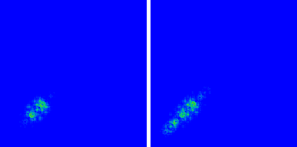
Figure 20: Density plot of two selected eigenstates for $U=4.5$, $U_{R}=1$ and for the rational approximations of $\alpha_{2}/(2\pi)$. The corresponding system sizes, energy eigenvalues and values for both types of inverse participation ratios are: Left: $N=369$, $E=-2.21758$, $\xi_{E}=11.378$, $\xi_{x}=21.029$ (2nd largest value of $\xi_{E}$ and largest value of $\xi_{x}$ for this system size and approximate energy). Right: $N=1605$, $E=-2.21949$, $\xi_{E}=16.367$, $\xi_{x}=26.748$ (largest value of $\xi_{E}$ for this system size and approximate energy). The left panel shows the full state of size $369\times 369$ and the right panel a zoomed region of size $369\times 369$ with left bottom corner at position $x_{1}=x_{2}=0$ and outside the zoomed range no data points different from blue (for zero amplitude) are visible.

We have also tested (for $\alpha_{2}$) the interaction strength $U=4.5$ with approximate energy $E=-3.1$ which provided nice FIKS pairs for the golden ratio case studied in Sec. 5. However, here we should not expect delocalized FIKS pairs since according to Fig. 15 the value of $\xi_{\rm IPR}$ obtained from the time evolution state is very small. On the other side, the variance length shows some modestly increased values and it might be useful to verify such cases as well. We applied the standard procedure of energy refinement with the Green function Arnoldi method on $U=4.5$ with the initial energy $E=-3.1$ which immediatedly selected $E\approx-2.2$ as “optimal” energy range (to maximize $\xi_{E}$). Despite some modestly delocalized eigenstates with $\xi_{E}\sim 15$ and $\xi_{x}\sim 25$ (for the largest considered systems sizes $N=412$, 1193 and 1605) there are no FIKS pairs with strong delocalization along the diagonal. Fig. 20 shows for $\alpha_{2}$ and $N=369$ or $N=1605$ two such modestly delocalized eigenstates which have some “cigar” form but with a rather short length $\sim 50$-$80$ and a rather elevated width $\sim 20$-$30$. It seems that the variance length, in contrast to $\xi_{\rm IPR}$, does not really allow to distinguish between these kind of states and nice FIKS eigenstates. Furthermore this example shows that suitable parameters $U$ and $E$ for FIKS states depend strongly on the flux parameter $\alpha$, an issue which is more systematically studied in the next Section.

9 Dependence on flux values

A problem with a systematic study of the dependence of the FIKS effect on different flux values is to select a suitable set of irrational numbers of comparable quality and which have roughly the same distance. For this we consider at first rational numbers $p/89$ with $44\leq p\leq 88$ where the denominator $89$ has the nice feature of being both a prime and a Fibonacci number. We compute for each of these rational numbers the canonical variant of its finite continued fraction expansion cf_rational , reduce the last coefficient by 1 and add an infinite sequence of entries of 1. This provides the infinite continued fraction expansion of an irrational number which is rather close to the initial fraction $p/89$ and which has “a golden tail” for the continued fraction expansion. It turns out that for each value of $p$ the difference between $p/89$ and the corresponding irrational number is approximately $5\times 10^{-5}$ therefore providing a nice data set of irrational numbers between 0.5 and 1.

In particular for $p=55$, where $55/89$ is a rational aproximation of the golden number, we have $55/89=[0;1,1,1,1,1,1,1,1,2]$. The procedure reduces the last coefficient from 2 to 1 and adds the infinite sequence of unit entries just providing exactly the continued fraction expansion of the golden number (with all coefficients being unity). The golden number is therefore one of the data points in the selected set of irrational numbers. For $p=64$ we find the irrational value $0.7191011235955056\ldots$ which is by construction very close to $64/89$ but also rather close to $266/369\approx 0.72087$, which was used in the experiment of Ref. bloch , and also to the two irrational numbers (22) and (8) used in the previous Section.

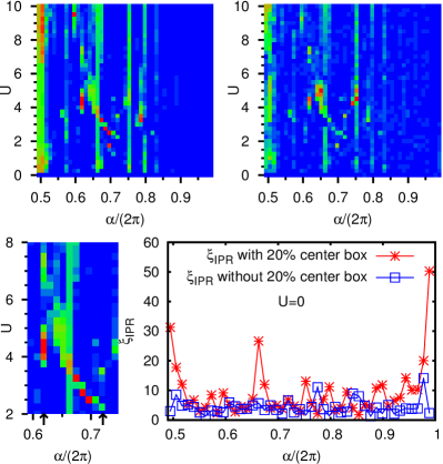
Figure 21: Top panels : Density plot of the squared tail norm $\|\psi_{\rm tail}(t)\|^{2}$ (left panel) or the inverse participation ratio computed without 20% center box (right panel) with horizontal axis representing the parameter $\alpha/(2\pi)$ and vertical axis representing the interaction strength $U$ using a time evolution state for system size $N=512$, iteration time $t=5120$, interaction range $U_{R}=1$ and a localized initial state for $t=0$ with both particles in the center position $x_{0}=N/2$. The bottom left panel shows a zoomed range with $0.6\leq\alpha/(2\pi)<0.75$ and $2\leq U\leq 8$ of the top left panel. The two arrows indicate the value of the golden ratio $\alpha/(2\pi)=(\sqrt{5}-1)/2\approx 0.618$ and the value $\alpha/(2\pi)=266/369\approx 0.721$ used in the experiments of Ref. bloch . The bottom right panel shows the inverse participation ratio for $U=0$ versus the parameter $\alpha/(2\pi)$ and computed with (red crosses) and without (blue squares) the 20% center box. The maximal value is for the squared tail norm $0.12519$ (for $\alpha\approx 0.596$ and $U=9.5$) and for the the inverse participation ratio without 20% center box $188.68$ (for $\alpha\approx 0.753$ and $U=4.5$). The data of this figure are obtained with $\beta=(\sqrt{5}-1)/2$ (and not $\beta=0$ as the data of Fig. 1 and Table 1 in Sec. 4).

Using these irrationals values for $\alpha/(2\pi)$ and $\beta=(\sqrt{5}-1)/2$ we have performed the time evolution analysis described in Sec. 4 for system size $N=512$, iteration time $t=5120$ and the interaction interval $0\leq U\leq 10$ in steps of $\Delta U=0.25$ providing in total $45\times 21$ data sets. The main results of this analysis are shown in Fig. 21 containing two density plots in $\alpha/(2\pi)$-$U$ plane for the squared tailed norm $\|\psi_{\rm tail}(t)\|^{2}$ and the inverse participation ratio $\xi_{\rm IPR}$ (without 20% center box) both providing the most reliable measure of delocalization in the framework of the time evolution analysis (the variance length provides a considerable amount of fluctuation peaks also when the other two quantities are very small as can be seen in Figs. 1 and 15).

Concerning the density plots of a quantity $\rho$ we mention that we apply the attribution of the different color codes to uniform slices of $\rho^{r}$ with $r\leq 1$ being some exponent, of typical choice $1/4$ or sometimes $1/8$, to increase the visibility of small values of $\rho$. In Fig. 21 we used for the density plot of the squared tail norm the standard choice $r=1/4$ due to the large ratio $\sim 10^{12}$ between maximum and minimum values but for $\xi_{\rm IPR}$ where this ratio is $\sim 10^{2}$ we chose exceptionnally $r=1$. For these plot parameters the density plots for these two quantities provide rather coherent and similar results for parameter regions with strong delocalization. All raw data of Fig. 21 are available for download at webpage .

The density plots of Fig. 21 show that for values of $\alpha/(2\pi)$ close to the simple fractions $1/2$, $2/3$, $3/4$ and even $4/5$ there is a certain rather uniform delocalization effect for nearly all interaction values $U>0$. We attribute this observation to a strong enhancement of the one particle location length even in absence of interaction for these flux values as can be seen in the bottom right panel of Fig. 21 which compares the two variants of the inverse participation ratio computed with or without the 20% center box for vanishing interaction strength $U=0$. The first variant of $\xi_{\rm IPR}$ measures rather directly the effective one-particle localization length and is quite enhanced for the above simple fractions if compared to the standard value $\ell=1/\log(\lambda)\approx 4.48$ for $\lambda=2.5$ (for irrational values of $\alpha/(2\pi)$ and infinite system size) aubry . It seems that for the irrational values close to simple fractions the system size $N=512$ is still too small to see this standard value and one observes an effective enhanced one-particle localization length. We have verified this also by direct diagonalization for some example cases.

Apart from the simple fractions there are certain combinations of $\alpha/(2\pi)$ and $U$ with a strong FIKS effect and a non-enhanced one-particle localization length. For exemple for the golden ratio case one recovers the peaks at $U=4.5$ and $U=7.25$ (being close to $7.2$ found in Sec. 4) and also for $\alpha/(2\pi)$ close to the value of $266/369$ of Ref. bloch there are two modest peaks of green color at $U=2.25$ and $U=3.5$ (being close to $3.6$ found in the previous Section) as can be seen from the zoomed density plot of the squared tail norm (bottom left panel in Fig. 15). We remind that the value $U=2.25$ also required longer iteration times ($t=10240$ instead of $t=5120$) to be more clearly visible thus explaining the green (instead of red) color for this data point since in Fig. 15 we have $t=5120$.

Other examples are $\alpha\approx 0.596$ and $U=9.5$ (with maximal value of the squared tail norm of all data sets), $\alpha\approx 0.753$ and $U=4.5$ (with maximal value of $\xi_{\rm IPR}$ without 20% center box) and $\alpha\approx 0.697$ with two interaction values $U=1.75$ and $U=2.5$. We also computed some eigenvectors by the Green function Arnoldi method for these four cases which clearly confirms the existence of FIKS eigenstates in each case. For example the strongest delocalized eigenstate for $\alpha\approx 0.596$, $U=9.5$ and $N=1533$ corresponds to $E=4.72729$, $\xi_{E}=426.076$, $\xi_{x}=324.511$ and for $\alpha\approx 0.753$, $U=4.5$ and $N=1837$ to $E=-0.68824$, $\xi_{E}=3618.270$, $\xi_{x}=955.650$.

We mention that, for the golden ratio value, the data of Fig. 21 are not perfectly identical/coherent to the data of Fig. 1 and Table 1 due to the different phase offset $\beta=0$ used for the latter.

10 Discussion

The results presented in this work clearly show the appearance of completely delocalized FIKS pairs induced by interaction in the non-interacting localized phase of the Harper model when all one-particle eigenstates are exponentially localized. The number of sites (states) $\xi$ populated by FIKS pairs grows with the system size approximately like a power law $\xi\propto N^{b}$ with the exponent being approximately in the range $0.7\leq b\leq 1$. We assume that the actual value of $b$ may depend on the energy range and interaction strength. It is possible that for $b<1$ we have some multi-fractal structure of FIKS eigenstates. In spite of a significant numerical progress and large system sizes studied here (we note that the total Hilbert space of the TIP problem is $N_{H}=N^{2}\approx 10^{8}$ at maximal $N=10946$) there are still many open aspects in this interesting problem of interplay of interactions, localization and quasiperiodicity. Below we list the main of them.

Physical origin of FIKS pairs. We see rather subtle and complex conditions for appearance of FIKS pairs. Their regions of existence are rather narrow on the energy interval, flux and in the range of interactions (see e.g. Figs. 8,21). However, at optimal parameters we may have up to $12\%$ of states from the initial configuration with particles on the same or nearby site being projected on FIKS pairs. Thus the optimal conditions and the physical understanding of the FIKS effect should be clarified. If the energy eigenvalue equation of the original Hamiltonian (1)-(5) is rewritten in the basis of non-interacting eigenstates then it gets the form dlsharper

$$(\epsilon_{m_{1}}+\epsilon_{m_{2}})\chi_{m_{1},m_{2}} + U\sum_{{m^{{}^{\prime}}_{1}},{m^{{}^{\prime}}_{2}}}Q_{m_{1},m_{2},{m^{{}^{\prime}}_{1}},{m^{{}^{\prime}}_{2}}}\chi_{{m^{{}^{\prime}}_{1}},{m^{{}^{\prime}}_{2}}}$$ (24)

$$= E\chi_{m_{1},m_{2}}$$

where $\chi_{m_{1},m_{2}}$ are eigenfunctions of the TIP problem in the basis of the non-interacting product states $|\phi_{m_{1}},\phi_{m_{2}}\!\!>$ introduced in Appendix B. Note that the (second variant) of the Green function Arnoldi method computes rather directly $\chi_{m_{1},m_{2}}$ and that $\xi_{E}$ is the inverse participation ratio in this energy representation. The transition matrix elements produced by the interaction are (for the Hubbard interaction case)

$$Q_{m_{1},m_{2},{m^{{}^{\prime}}_{1}},{m^{{}^{\prime}}_{2}}}=\sum_{x}\phi^{*}_{m_{1}}(x)\,\phi^{*}_{m_{2}}(x)\,\phi_{m^{{}^{\prime}}_{1}}(x)\,\phi_{m^{{}^{\prime}}_{2}}(x)\,$$ (25)

with $\phi_{m}(x)=<\!x|\phi_{m}\!>$ being the one-particle eigenfunctions of (1) with the one-particle energies $\epsilon_{m}$.

We know that one-particle energies of the Harper model at $\lambda>2$ have gaps and localized eigenstates. We can assume that the sum of TIP energies also has gaps (or quasi-gaps) and thus there are some narrow FIKS bands with TIP energy width $\lambda_{\rm eff}$. On the other side the interaction generates some transition matrix elements between these band states with a certain typical transition amplitude $t_{\rm eff}\propto U$. Since the energy inside the FIKS band oscillates quasiperiodically with the distance along the lattice we can have approximately the situation of the original Aubry-André model so that the delocalization transition will take place as soon as $\lambda_{\rm eff}<2t_{\rm eff}$. We think that this is the physical mechanism of TIP delocalization in the Harper model. However, the concrete verification of this mechanism is not so simple: the matrix elements are also oscillating with the lattice distance and there are quite a several of them (and not only two as in the Harper model), there are also energy shifts produced by interaction (the diagonal terms) and probably these shifts are at the origin of narrow regions of interaction where the FIKS pairs appear.

There are some indications from the kicked Harper model lima ; ketzmerick1999 ; prosenprl ; artuso , that coupling transitions between a large number of sites leads to new effects and even ballistic delocalized states. Such ballistic states appear in the regime when the classical dynamics is chaotic and diffusive and from the analogy with the quantum Chirikov standard map chirikovscholar one would expect to find only pure point spectrum of exponentially localized sates. Indeed, there are only two transition elements between sites in the Harper model while in the kicked Harper model there are several of them. The results presented here also indicate that the interactions with a longer range have a larger fraction of FIKS pairs. Thus for $U_{R}=5$, which has an optimal interaction range, comparable with the one-particle localization length, we obtain a rather large weight of FIKS pairs of about $10\%$ in energy and $10\%$ in the interaction range $0<U<20$ (see Figs. 1,8,11). These fractions exceed significantly the typical interaction and energy ranges for FIKS pairs with the Hubbard interaction.

We assume that the spectrum of FIKS pairs has a structure similar to the spectrum of the delocalized phase in the Aubry-André model at $\lambda<2$, being close to the ballistic spectrum. Indeed, in the time evolution of wave packet (see e.g. Fig. 3) we see the lines with a constant slope corresponding to a ballistic propagation with a constant velocity. The maximal velocity is $v_{p}\approx x_{\rm max}/t_{\rm min}\approx 0.2$ being smaller then the maximal velocity $v_{p}=1$ for one particle at $\lambda=0$. It is clear that much more further work should be done to obtain a deeper physical understanding of the FIKS effect in the Harper model.

Mathematical aspects. The question about the exact spectral structure of FIKS pairs is difficult to answer only on the basis of numerical simulations since the system size remains always finite and subtle fractal properties of the spectrum require more rigorous treatment. There are significant mathematical advancements in the analysis of quasiperiodic Schrödinger operators reported in lana1 ; lana2 ; lana3 . We hope that the results presented here will stimulate mathematicians to the analysis of properties of the FIKS phase.

FIKS pairs in cold atom experiments. The results presented in Sec. 8 show that the FIKS pairs exists at the irrational flux value $\alpha/(2\pi)\approx 532/738$ realized in the recent experiments bloch . However, the initial state prepared in bloch had approximately one atom per each second site thus being rather far from the initial configuration considered here. We think that an initial state with all atoms located in the center of the lattice will be much more favorable for the observation of FIKS pairs. Indeed, such a state is rather similar to the initial state considered in our paper (two particles on same on nearby sites) and thus we expect that in the experiments one will see ballistic propagating FIKS pairs on the tails of probability distribution like it is well seen in Figs. 16, 17.

We note that the initial state with all atoms in the center of the lattice had been used in cold atoms experiments in the regime of the Aubry-André model modugno . In these experiments a subdiffusive delocalization of wave packet has been observed being similar to the numerical studies of the nonlinear Schrödinger equation on the disordered lattice. Indeed, in the center of the packet with many atoms the Gross-Pitaevskii description can be more adequate comparing to the TIP case considered here. However, on the tails of probability distribution on larger distances from the center there are only a few atoms and only FIKS pairs can reach such far away distances. Thus it is rather possible that the probability tails will contain mainly FIKS pairs. In fact the experimental data in modugno (Fig. 3a there) have a plateau of probability at large distances. However, at present it is not clear if this is an effect of fluctuations and experimental imperfections or a hidden effect of FIKS pairs. We think that the present techniques of experiments with cold atoms in quasiperiodic lattices allow to detect experimentally the FIKS pairs discussed in this work.

FIKS pairs for charge-density wave and high $T_{c}$ materials. We can expect that at finite electron density in a 1D potential at certain conditions the main part of electrons below the Fermi energy will remain well localized creating an incommensurate quasiperiodic potential for a small fraction of electrons in a vicinity of the Fermi level. The FIKS pairs can emerge for this fraction of electrons. Such situations can appear in the regime of charge-density wave in organic superconductors and conductors at incommensurate electron density created by doping (see e.g. lebed ). In such a regime it is possible that the FIKS pairs will give a significant contribution to conductivity in such materials. The proximity between the charge-density wave regime and high $T_{c}$ superconductivity in cuprates kivelson1 ; kivelson2 also indicates a possibility that FIKS pairs can play a role in these systems. However, a more detailed analysis of finite density systems is required for the solid state systems.

We think that the various aspects of possible implications of FIKS pairs in various mathematical and physicals problems demonstrate the importance of further investigations of this striking phenomenon.

This work was granted access to the HPC resources of CALMIP (Toulouse) under the allocation 2015-P0110.

Appendix A Description of the Arnoldi method

For both Lanczos and Arnoldi methods one chooses some initial vector $|\zeta_{1}\!>$, which should ideally contain many eigenvector contributions, and determines a set of orthonormal vectors $|\zeta_{1}\!>\,\ldots,\,|\zeta_{n_{A}}\!>$, where we call $n_{A}$ the Arnoldi dimension, using Gram-Schmidt orthogonalization on the vector $H|\zeta_{k}\!>$ with respect to $|\zeta_{1}\!>\,\ldots,\,|\zeta_{k}\!>$ to obtain $|\zeta_{k+1}\!>$. This scheme has to be done for $k=1,\,\ldots,\,n_{A}$ and it also provides an approximate representation matrix of “modest” size $n_{A}\times n_{A}$ of $H$ on the Krylov subspace generated by these vectors. The largest eigenvalues of this representation matrix, also called Ritz eigenvalues, are typically very accurate approximate approximations of the largest eigenvalues of $H$ and the method also allows to determine (approximate) eigenvectors. It requires that the product of $H$ to an arbitrary vector can be computed efficiently, typically for sparse matrices $H$ but, as we will see in the next Section, even non-sparse matrices such as resolvent operators can be used provided an efficient algorithm for the matrix vector product is available.

In its basic variant the Arnoldi method provides only the eigenvalues and eigenvectors for the largest energies (in module) at the boundary of the band which is not at all interesting and in our case it is indeed necessary to be able to determine accurately the eigenvalues close to a given arbitrary energy.

The standard method to determine numerically a modest number of eigenvalues localized in a certain arbitrary but small region of the eigenvalue space for generic large sparse matrices is the implicitly restarted Arnoldi method. In this method the initial vector is iteratively refined by removing eigenvector contributions whose eigenvalues are outside the energy interval of interest using a subtle procedure based on shifted QR-steps stewart . Using this algorithm we have been able to determine eigenvalues and eigenvectors for system sizes up to $N=700$-$1000$ but the computation time is very considerable due to the large number of iterations to achieve convergence of eigenvectors. Furthermore, in order to limit the computational time to a reasonable amount one has to accept eigenvalues of modest quality with $\delta^{2}E(\psi)=10^{-12}$-$10^{-8}$ where the quantity

$$\delta^{2}E(\psi)=<\!\psi|\,(E-H)^{2}\,|\psi\!>$$ (26)

measures the quality of an approximate eigenvector $|\psi\!>$ with an approximate eigenvalue $E=<\!\psi|\,H\,|\psi\!>$. Writing $|\psi\!>=|\psi_{\rm exact}\!>+\varepsilon|\delta\psi\!>$ with $H|\psi_{\rm exact}\!>=E_{\rm exact}|\psi_{\rm exact}\!>$ and $\|\delta\psi\|=1$ one finds easily that $<\!\psi_{\rm exact}|\delta\psi\!>={\cal O}(\varepsilon^{2})$ (due to normalization of $|\psi\!>$ and $|\psi_{\rm exact}\!>$) and therefore $E=E_{\rm exact}+{\cal O}(\varepsilon^{2})$ and $\delta^{2}E(\psi)={\cal O}(\varepsilon^{2})$. Therefore a value of $\delta^{2}E(\psi)=10^{-8}$ implies $\varepsilon\sim 10^{-4}$.

Appendix B Details of the Green function Arnoldi method

In this appendix we provide some of the details concerning the Green function Arnoldi method. For the sake of simplicity, we will omit (most of) the details concerning the (anti-)symmetrization of two-particle states for bosons (fermions) and the corresponding matrix operators acting on them. These details are of course important and must be dealt with care and precision when implementing the algorithm. For example, the efficient algorithm for the position-energy transformation (see below) requires a temporary extension of (anti-)symmetrized states of the boson (fermion) space of dimension $N_{2}$ to states in the general non-symmetrized two-particle space of dimension $N^{2}$ and a corresponding reduction afterwards. However, the details for this kind of extensions or reductions with eventual $\sqrt{2}$ factors etc. are based on the application of basic text book quantum mechanics and would only obscure the following description.

Our algorithm exploits the fact that the interaction operator $\hat{U}$ acts only on a small number of sites $(2U_{R}-1)\,N\ll N^{2}$ U_R given by the set

$$S=\Bigl{\{}(x_{1},x_{2})\ \Big{|}\ |x_{1}-x_{2}|<U_{R}\Bigr{\}}$$ (27)

(see again U_boundary ). Let us denote by

$$P=\sum_{(x_{1},x_{2})\in S}|x_{1},x_{2}\!><\!x_{1},x_{2}|.$$ (28)

the projector on the sites belonging to the set $S$. Obviously $P$ commutes with the interaction operator $\hat{U}$ given in (5) and we have $P\hat{U}P=P\hat{U}=\hat{U}P=\hat{U}$. For the case of the Hubbard interaction with $U_{R}=1$ we even have $\hat{U}=UP$ where $U$ is the interaction strength and corresponds to the situation considered in vonoppen ; frahm_tip_green . However for $U_{R}>1$ and $w>0$ we note that the operators $\hat{U}$ and $P$ are not proportional (but of course they still commute). We denote by $H_{0}=h^{(1)}+h^{(2)}$ the Hamiltonian in absence interaction and by $G_{0}=(E-H_{0})^{-1}$ the Green function or resolvent of $H_{0}$. Furthermore we denote by $\bar{G}_{0}=PG_{0}P$ the projected resolvent (for $U=0$) which is a non-trivial (non-zero) operator only with respect to its diagonal block associated to the subspace corresponding to the set $S$.

In this case we can state the following “magic” exact formula (6) which is the basic ingredient of our numerical approach. This formula can be obtained from a perturbative expansion of $G$ with the interaction as perturbation and an exact resummation of all terms except the first one. It is also possible to provide an algebraic direct proof without use of an expansion and we insist on the fact that (6) is exact and not approximate. Details for both derivations are given in Appendix C.

The key for an efficient determination of $G|\varphi\!>$ using (6) is the observation that the operator $({\bf 1}-\hat{U}\bar{G}_{0})^{-1}\hat{U}$ applied to any vector provides only non-zero contributions on the subspace associated to the set $S$ and the matrix inverse is done for a matrix of size $U_{R}N\ll N_{2}$ [or $(U_{R}-1)N\ll N_{2}$ for the fermion case] G0 once $\bar{G}_{0}$ has been determined. This approach generalizes an idea already used in vonoppen ; frahm_tip_green where (for the case of Hubbard interaction) the projected resolvent (for arbitrary $U$) $\bar{G}=PGP=\bar{G}_{0}\,({\bf 1}-\hat{U}\bar{G}_{0})^{-1}$ was calculated to determine the localization properties of two interacting particles in one dimension from $\bar{G}$ (we remind that in vonoppen ; frahm_tip_green a disorder and not quasiperiodic potential was studied).

The numerical algorithm to determine efficiently $G|\varphi\!>$ is composed of two parts. The first part is to calculate $\bar{G}_{0}$ and the matrix inverse $({\bf 1}-\hat{U}\bar{G}_{0})^{-1}$ which needs to be done only once if the value of $E$ is not changed. The second part is to evaluate efficiently the successive matrix vector products (with $G_{0}$, $\hat{U}$, $({\bf 1}-\hat{U}\bar{G}_{0})^{-1}$ etc.) accordingly to the formula (6).

For both parts we need first to diagonalize the one-particle Hamiltonian $h$ resulting in eigenvectors $|\phi_{\nu}\!>$ and eigenvalues $\epsilon_{\nu}$ which can be done with complexity ${\cal O}(N^{3})$ (or even better using inverse vector iteration for the eigenvectors). Then the resolvant $G_{0}$ can be determined from

$$<\!x_{1},x_{2}| G_{0} |y_{1},y_{2}\!>=\sum_{\nu,\mu}\frac{\phi_{\nu}(x_{1})\,\phi_{\mu}(x_{2})\,\phi_{\mu}(y_{2})\,\phi_{\nu}(y_{1})}{E-\epsilon_{\nu}-\epsilon_{\mu}}$$ (29)

$$= \sum_{\nu}\phi_{\nu}(x_{1})\,g(E-\epsilon_{\nu};x_{2},y_{2})\,\phi_{\nu}(y_{1}),$$

$$g(E;x,y) = \sum_{\mu}\frac{\phi_{\mu}(x)\,\phi_{\mu}(y)}{E-\epsilon_{\mu}}=<\!x|(E-h)^{-1}|y\!>$$ (30)

where $g(E;x,y)$ is the one-particle Green function and $\phi_{\nu}(x)=<\!x|\phi_{\nu}\!>$.

We use (29) to determine the projected resolvent $\bar{G}_{0}$, i. e. for $(x_{1},x_{2}),\,(y_{1},y_{2})\in S$. This requires only ${\cal O}(N^{3}\,U_{R}^{2})$ operations in total since for each value of $\nu$ we can determine the one-particle Green function as inverse of a tridiagonal matrix (with periodic boundary conditions) with ${\cal O}(N^{2})$ operations using a smart formulation of Gauss algorithm. Then, still for the same value of $\nu$, we have to update the sums for all possible values $(x_{1},x_{2}),\,(y_{1},y_{2})\in S$ which costs ${\cal O}(N^{2}\,U_{R}^{2})$ operations which is dominant (or comparable if $U_{R}=1$) to the complexity of the one-particle Green function evaluation. The sum/loop over $\nu$ leads then to a further factor of $N$ giving ${\cal O}(N^{3}\,U_{R}^{2})$ operations. The subsequent matrix inverse to determine $({\bf 1}-\hat{U}\bar{G}_{0})^{-1}$ requires ${\cal O}(N^{3}\,U_{R}^{3})$ operations. We mention that for the Hubbard interaction case $U_{R}=1$ this algorithm to determine $\bar{G}_{0}$ and the inverse was already implemented and explained in Ref. frahm_tip_green .

For the second part of the algorithm we still need an efficient method to evaluate $G_{0}|\varphi\!>$ for a given vector $|\varphi\!>$. This can actually be done by a transformation from position to energy representation, i. e. an expansion of $|\varphi\!>$ using the eigenvectors of $H_{0}$ given as product states $|\phi_{\nu},\phi_{\mu}\!>$. This transformation can be done with essentially ${\cal O}(N^{3})$ operations using the trick to transform first the coordinate of the first particle and then in a separate subsequent step the coordinate of the second particle. Each one-particle transformation requires ${\cal O}(N^{2})$ operations but it has to be done for $N$ possible positions of the other particle and the transformation for the other particle gives a further factor of 2 resulting in $\sim 2N^{3}$ addition and multiplication operations for one two-particle transformation. The transformation back into position representation can be done similarly.

Since $G_{0}$ is diagonal in the energy representation (with eigenvalues $(E-\epsilon_{\nu}-\epsilon_{\mu})^{-1}$) the product $G_{0}|\varphi\!>$ in this representation only requires ${\cal O}(N^{2})$ operations. Once this is done the resulting vector is transformed back into position representation (also with ${\cal O}(N^{3})$ operations). Then the product of the matrix $({\bf 1}-\hat{U}\bar{G}_{0})^{-1}\hat{U}$ to a vector in position representation only requires ${\cal O}(N^{2}U_{R}^{2})$ operations (provided that the matrix inverse is calculated and stored only once in advance for a fixed value of $E$). Finally a further double-transformation-multiplication step with $G_{0}$ is necessary. Combing all this it is possible to evaluate $G|\varphi\!>$ by (6) by ${\cal O}(N^{3})$ operations (but with a rather big prefactor) where the most complex part consists of the two position-energy transformations and the two inverse energy-position transformations.

In summary we have described an algorithm to determine $G|\varphi\!>$ by ${\cal O}(N^{3}\,U_{R}^{3})$ operations for the initial preparation for a given energy $E$ and ${\cal O}(N^{3})$ operations for each product (i. e. $G$ applied to several different vectors) provided the initial value of $E$ is not changed. In terms of the matrix size $N_{2}\approx N^{2}/2$ this implies a complexity of ${\cal O}(N_{2}^{3/2})$ operations which is more expensive than the product $H|\varphi\!>$ with ${\cal O}(N_{2})$ operations but still much better than the naive matrix vector multiplication with ${\cal O}(N_{2}^{2})$ operations.

The position-energy transformation can be furthermore optimized for larger system sizes using that the one-particle eigenfunctions $\phi_{\nu}(x)$ are localized around some position $x_{\rm max}$ with localization length $\ell$. In this case the ratio $|\phi_{\nu}(x)/\phi_{\nu}(x_{\rm max})|$ is below $10^{-17}$ (the numerical rounding error for standard double precision numbers) for $|x-x_{\rm max}|>c$ with the constant $c=17\,\log(10)\,\ell\approx 175$ if we replace the value $\ell\approx 4.48$ for $\lambda=2.5$. The positions $x$ fulfilling this condition can be safely excluded in the multiple sums for the position-energy transformation therefore reducing the complexity to ${\cal O}(c\,N^{2})$.

This first variant of the algorithm combined with the (simple) Arnoldi method for $G$ is already very efficient and very superior to the implicitly restarted Arnoldi method applied to $H$ and produces for a sufficiently large value of the Arnoldi dimension $n_{A}$ easily more than $50\%-70\%$ of numerically accurate eigenvalues close to the energy $E$ appearing in the Green function (from all $n_{A}$ Ritz eigenvalues produced by the Arnoldi method). For example for the Hubbard case with $U=7.8$ and $E=-2.78$ we have been able, on a machine with 64 GB of RAM memory, to increase the system size up to $N=4181$ (which is a Fibonacci number) and to choose the Arnoldi dimension $n_{A}=900$ and about 620 out of 900 obtained eigenvalues have a quality with $\delta^{2}E(\psi)<10^{-20}$ quality . Furthermore most of the important parts of the algorithm can be quite well parallelized for multiple core machines.

As start vector for the Arnoldi iteration we choose a vector proportional to the projection $P\sum_{x_{1},x_{2}}|x_{1},x_{2}\!>$, i. e. a vector with uniform identical values for the sites in the set $S$ where the interaction acts. In this way we avoid (most of) the many useless contributions from eigenstates which are essentially localized product states $|\phi_{\nu},\phi_{\mu}\!>$ with both particles localized very far away such that the interaction has no effect on them. With this start vector we capture all well “delocalized” states with energies close to the value of $E$. The Arnoldi method still provides a considerable number of eigenstates being similar to strongly localized product states where the distance between particles is “modest”, i. e. sufficiently large that the product states are indeed relatively good eigenstates of $H$ but also sufficiently small that the initial vector has small contributions of these states which will be amplified by the Green function Arnoldi method if the eigenvalue of the product state is sufficiently close to $E$.

For small values of $U_{R}$ the memory requirement of the Arnoldi method is determined by the number $n_{A}$ of iteration vectors which need to be stored and the size of these vectors $N_{2}\approx N^{2}/2$ which provides the essential limitation of this method concerning the choice of $n_{A}$ and $N$. For larger values of $U_{R}$, e. g. $U_{R}=20$ the largest value we have considered, the requirement to store multiple matrices of size $U_{R}N\times U_{R}N$ is also important (or even dominant for the second variant described below).

However, this first variant of the Green function Arnoldi method, which works with vectors stored in the position representation, can be considerable improved by using vectors stored in the non-interaction energy representation using an expansion in terms of the non-interacting product states $|\phi_{\nu},\phi_{\mu}\!>$. This modification allows for several improvements.

First, the number of the rather expensive energy-position (or inverse position-energy) transformation steps is reduced from four to two when evaluating $G|\varphi\!>$ since, according to the above description of the algorithm, the first energy-position and the last inverse position-energy transformation can be avoided if the vector $|\varphi\!>$ is by default already available (or needed) in energy representation (instead of position representation).

Second, in this modified variant it is natural to choose a somewhat different start vector, i. e. a vector given as sum of product states with maximal positions in the set $S$ which is qualitatively similar to the other initial vector used for the first variant but still different due to the finite one-particle localization length. The important point is that the new initial vector contains less contributions from useless products states. For given values of $n_{A}$ and $N$ this improves considerably the quality of the eigenvectors by reducing the value of the quantity (26) and one obtains more nicely “delocalized” states (with eigenvalues a bit further away from $E$) and less useless product states.

The third improvement concerns the possibility to reduce considerably the dimension of the Hilbert space in energy representation from $N_{2}\approx N^{2}/2$ to $cN$ (with $c\approx 175$ for $\lambda=2.5$) since one can simply remove all product states with maximal positions further away than $c$ because these states do not feel the interaction at all (i. e. with interaction coupling matrix elements smaller than $10^{-17}$). This reduces the amount of memory usage and also computation time for the Arnoldi iterations by a factor $2c/N$ which becomes quite small for large system sizes ($N>1000$). Especially the reduced memory requirement allows to perform computations with larger values of $N$ and $n_{A}$, for example for $U_{R}=1$ we have been able to choose a system size $N=10946$ with Arnoldi dimension $n_{A}=3000$ (on a machine with 64 GB of RAM memory). For the case $N=4181$ and $n_{A}=900$, the maximum possible size for the first variant with 64 GB, the computation time for the second variant of the method is reduced by a factor of ten if compared to the first variant.

The overall complexity of the Green function Arnoldi method for small systems ($N\leq c$) is given by $C_{1}(U_{R}N)^{3}+C_{2}N^{3}\,n_{A}+C_{3}N^{2}\,n_{A}^{2}$ with three terms representing the initial preparation part (first term with the constant $C_{1}\sim 1$), the Green function vector multiplications (second term with the constant $C_{2}\sim 5$) and the Gram-Schmidt orthogonalization scheme (third term with the constant $C_{3}\sim 1$). For larger systems $N\gg c=175$ we have to replace in the second and third term a factor of $N$ by $c$ resulting in $C_{1}(U_{R}N)^{3}+C_{2}\,c\,N^{2}\,n_{A}+C_{3}\,c\,N\,n_{A}^{2}$. If one choose typically $n_{A}\sim N$ the second and third term have comparable complexity $\sim c\,N^{3}$ but in practice the second term is dominant due to a considerably larger value of the constant $C_{2}$. Therefore it is not interesting to use the Lanczos method (instead of the full Arnoldi iterations) because this would only remove in the last, non-dominant, term one factor of $N$. The memory requirements (in units of size of double precision numbers) scale with $C_{4}\,(U_{R}N)^{2}+C_{5}\,c\,N\,n_{A}$ with $C_{4}\sim 5C_{5}$ and $C_{5}\sim 1$ because one has to store several copies of matrices of size $(U_{R}N)\times(U_{R}N)$ and $n_{A}$ vectors of size $c\,N$ for the Arnoldi iterations.

With increasing values of the interaction range $U_{R}$ the memory requirement and also computation time of the initial preparation part become more important or dominant, for $U_{R}=20$, but even for this extreme case we have been able to push the system size up to $N=1597$ and one can (should) choose very large values for $n_{A}$ for the second Arnoldi-iteration part to better exploit the computational “investment” of the preparation part. Even with $n_{A}=2500$ for $N=1597$ the second and third part require only about 5% of the computation time while for $U_{R}=1$ the first preparation part is typically negligible (at most 7% for the largest system size $N=10946$, $n_{A}=3000$ we considered).

We close this Appendix mentioning that the effective algorithm to compute arbitrary resolvent vector products can also be used to calculate more directly (or improve) individual eigenvectors if the eigenvalue (or an approximate eigenvector) is known with sufficient precision by the method of inverse vector iteration. We have for example been able to improve the modest quality eigenvectors which we had obtained by the implicitly restarted Arnoldi method to maximum possible precision only using a few number of these iterations. Actually, also a random initial vector can be used if a rather good approximate eigenvalue is known. However, to achieve a good efficiency for a systematic computation of many eigenvectors with close energies the Arnoldi method for the resolvent is the best choice to exploit the Green function algorithm. The reason is the expensive initial part of the algorithm [the rather expensive initial computation of $\bar{G}_{0}$ and the matrix inverse in (6)] which is only done once for the Arnoldi method and has to be repeated for any new individual eigenvalue when using inverse vector iteration.

Appendix C Projected Green’s function formula

In this appendix we show the formula (6) where $G=(E-H)^{-1}$, $G_{0}=(E-H_{0})^{-1}$, $H=H_{0}+\hat{U}$, $\bar{G}_{0}=PG_{0}P$ and $P=P^{2}$ is a projector such that $\hat{U}=P\hat{U}=\hat{U}P=P\hat{U}P$, i. e. $\hat{U}$ has the same eigenvectors as $P$ and only non-vanishing eigenvalues if the corresponding eigenvalue of $P$ is unity.

C.1 Perturbative expansion of $G$

The proof of (6) by an expansion in a matrix power series is quite illustrative. First we express $G$ as

$$G = \Bigl{[}({\bf 1}-\hat{U}G_{0})(E-H_{0})\Bigr{]}^{-1}$$ (31)

$$= G_{0}({\bf 1}-\hat{U}G_{0})^{-1}=G_{0}\sum_{n=0}^{\infty}(\hat{U}G_{0})^{n}$$

$$= G_{0}+G_{0}\left(\sum_{n=0}^{\infty}(\hat{U}G_{0})^{n}\right)\hat{U}G_{0}$$ (32)

where we have assumed that the matrix power series converges well which is the case for sufficiently large values of $E$ in the complex plane. Using the relations between $\hat{U}$ and $P$ we may rewrite the expression (32) as:

$$G=G_{0}+G_{0}\left(\sum_{n=0}^{\infty}(\hat{U}PG_{0}P)^{n}\right)\hat{U}G_{0}$$ (33)

which becomes after replacing $\bar{G}_{0}=PG_{0}P$ and resumming the series (in parentheses) just formula (6). Furthermore applying an argument of analytic continuation the validity of (6) is extended to all values of $E$ in the complex plane (except the singularities of $G$ or $G_{0}$). This calculation shows the crucial role of the relations between the interaction operator $\hat{U}$ and the projector $P$ and which finally allow to reduce the difficulty to determine the resolvent $G$ by using a matrix inverse in a subspace of considerably smaller dimension which is just the subspace onto which $P$ projects.

C.2 Algebraic direct proof

The expansion in a matrix power series and the argument of analytic continuation can be avoided by a direct but somewhat “less clear” calculation. For this we write:

$$G = G(E-H_{0})G_{0}=G(E-H+\hat{U})G_{0}=G_{0}+G\hat{U}G_{0}$$ (34)

$$= G_{0}+G_{0}({\bf 1}-\hat{U}G_{0})^{-1}\hat{U}G_{0}$$

$$= G_{0}+G_{0}\hat{O}\hat{U}G_{0}$$ (35)

where we have used the first identity of (31) to obtain (34). The operator $\hat{O}$ is given by $\hat{O}=(1-PA)^{-1}P$ and $A=\hat{U}G_{0}$ and to obtain (35) we have used (twice) that $P\hat{U}=\hat{U}$. We rewrite $\hat{O}$ in the form

$$\hat{O}=({\bf 1}-PA)^{-1}P({\bf 1}-PAP)({\bf 1}-PAP)^{-1}$$ (36)

and since $P({\bf 1}-PAP)=({\bf 1}-PA)P$ we obtain the expression

$$\hat{O}=P({\bf 1}-PAP)^{-1}=({\bf 1}-PAP)^{-1}P=({\bf 1}-\hat{U}\bar{G}_{0})^{-1}P$$

which together with (35) (and again $P\hat{U}=\hat{U}$) provides the formula (6).

References

- (1) P.G. Harper, Proc. Phys. Soc. London Sect. A 68, 874 & 879 (1955).
- (2) M.Y. Azbel, Sov. Phys. JETP 19, 634 (1964).
- (3) D.R. Hofstadter, Phys. Rev. B 14, 2239 ̵͑(1976).
- (4) S. Aubry and G. André, Ann. Israel Phys. Soc. 3, 133 (1980).
- (5) S.Y. Jitomirskaya, Ann. Math. 150, 1159 (1999).
- (6) J.B. Sokoloff, Phys. Rep. 126, 189 (1985).
- (7) T. Geisel, R. Ketzmerick, and G. Petschel, Phys. Rev. Lett. 66, 1651 (1991).
- (8) M. Wilkinson, and E.J. Austin, Phys. Rev. B 50, 1420 (1994).
- (9) D.L. Shepelyansky, Phys. Rev. B 54, 14896 (1996).
- (10) A. Barelli, J. Bellissard, Ph. Jacquod, and D.L. Shepelyansky, 77, 4752 (1996).
- (11) G. Dufour, and G. Orso, Phys. Rev. Lett. 109, 155306 (2012).
- (12) D.L. Shepelyansky, Phys. Rev. Lett. 73, 2607 (1994).
- (13) Y.Imry, Europhys. Lett. 30, 405 (1995).
- (14) D. Weinmann, A. Müller–Groeling, J.-L. Pichard, and K. Frahm, Phys. Rev. Lett. 75, 1598 (1995).
- (15) K. Frahm, A. Müller–Groeling, J.-L. Pichard, and D. Weinmann, Europhys. Lett. 31, 169 (1995).
- (16) F. von Oppen, T. Wetting, and J. Müller, Phys. Rev. Lett. 76, 491 (1996).
- (17) K.M. Frahm, Eur. Phys. J. B, 10, 371 (1999).
- (18) S. Flach, M. Ivanchenko, and R. Khomeriki, Europhys. Lett. 98, 66002 (2012).
- (19) G. Roati, C. D‘Errico, L. Fallani, M. Fattori, C. Fort, M. Zaccanti, G. Modugno, M. Modugno, and M. Inguscio, Nature 453, 895 (2008).
- (20) E. Lucioni, B. Deissler, L. Tanzi, G. Roati, M. Zaccanti, M. Modugno, M. Larcher, F. Dalfovo, M. Inguscio, and G. Modugno, Phys. Rev. Lett. 106, 230403 (2011).
- (21) M. Schreiber, S.S. Hodgman, P. Bordia, H. Lüschen, M.H. Fischer, R. Vosk, E. Altman, U. Schneider, and I. Bloch, Science 349, 842 (2015).
- (22) In view of the periodic boundary conditions the condition is understood to be true also for the case , i. e. if is close to one boundary and to the other boundary.
- (23) W.E. Arnoldi, Quart. Appl. Math. 9, 17 (1951).
- (24) G. W. Stewart, Matrix Algorithms Volume II: Eigensystems, SIAM (2001).
- (25) K.M. Frahm, and D.L. Shepelyansky, Eur. Phys. J. B 76, 57 (2010).
- (26) The Lanczos method is theoretically more efficient than the Arnoldi method since it requires only orthogonalization with respect to two and not all previous orthonormal vectors. However, this mathematical property is numerically problematic and may lead to the appearance of additional incorrect eigenvalues also know as “ghosts”. In this work, we used the less problematic but somewhat more “expensive” Arnoldi method, since the gain of efficiency of the Lanczos method is finally not relevant due to other parts in our numerical approach with a higher complexity. In view of this we speak in this work only of the Arnoldi method.
- (27) The expression for the number of sites in the set does not take into account the reduction of dimension due to (anti-)symmetrization. Of course for the boson (fermion) case there are only [] physical (anti-)symmetrized states associated to the set .
- (28) The projected resolvent takes a block diagonal form for the boson and fermion cases and when expressed in a basis of (anti-)symmetrized states. Therefore the matrix inverse involving can be done for a matrix size [] for bosons (fermions) and does not require a matrix size . To keep the discussion simple the details of these complications are omitted in Appendix B.
- (29) In all our programs, based on different variants or algorithms, the quality of obtained eigenvectors was checked independently by calculating the quantity (26) using the direct matrix vector multiplication of the sparse matrix with the numerically obtained eigenvector.
- (30) M. Frigo, A Fast Fourier Transform Compiler, Proc. 1999 ACM SIGPLAN Conf. “Programming Language Design and Implementation (PLDI ’99)”, Atlanta, Georgia, http://www.fftw.org/pldi99.pdf May 1999.
- (31) http://www.quantware.ups-tlse.fr/QWLIB/fikspairs
- (32) For each rational number there are two possible finite continued fraction expansions, one where the last coefficient is and the other one with one additional coefficient which is and where the second last coefficient is reduced by . We choose the first variant which is also called the canonical representation.
- (33) R. Lima, and D.L. Shepelyansky, Phys. Rev. Lett. 67, 1377 (1991).
- (34) R. Ketzmerick, K. Kruse, and T. Geisel, Physica D 131, 247 (1999).
- (35) T. Prosen, I. I. Satija, and N. Shah, Phys. Rev. Lett. 87, 066601 (2001).
- (36) R. Artuso, Scholarpedia 6(10), 10462 (2011).
- (37) B. Chirikov, and D.L. Shepelyansky, Scholarpedia 3(3), 3550 (2008).
- (38) J. Bourgain, and S. Jitomirskaya, Invent. math. 148, 453 (2002).
- (39) S. Jitomirskaya, and C.A. Marx, http://arxiv.org/abs/1503.05740 (2015)
- (40) A. Lebed (Ed.), The Physics of organic superconductors and conductors, Springer-Verlag, Berlin (2008).
- (41) E. Fradkin, and S. Kivelson, Nature Physics 8, 865 (2012).
- (42) B. Keimer, S.A. Kivelson, M.R. Norman, S. Uchida, and J. Zaanen, Nature 518, 179 (2015).