Interference Effect on Resonance Studies in Searches of Heavy Particles

Abstract

The interference between resonance signal and continuum background can be either constructive or destructive, depending on the relative sign of couplings between the signal and background amplitudes. Different interference schemes lead to asymmetric distortions of the resonance line shape, which could be distinguished in experiments, when the internal resonance width is larger than the detector resolution. Interpreting the ATLAS diboson excesses by means of a toy $W^{\prime}$ model as an illustrative example (though it is disfavored by the 13 TeV data), we find that the signs of resonance couplings can only be revealed in the line shape measurements up to a high confidence level at a high luminosity, which could bring us further information on the underlying theory beyond resonance searches at future lepton and hadron colliders.

I Introduction

The presence of a massive particle always manifests itself at high energy colliders as a resonance peak or significant excess over the (smooth) continuum background, if the decay products from the resonance particle can be reconstructed to some extent. The bound states of heavy quarks, top quark, $W$ and $Z$ bosons, and the 125 GeV standard model (SM) like Higgs are all observed in such a quantum manner. Taking into consideration both the production and decay processes, different helicity states of the resonance particle might interfere with each other Buckley:2007th ; Buckley2 ; Keung:2008ve ; Murayama:2014yja ; Cao:2009ah . It is more common that the the signal resonance interferes with the continuum background, as on colliders backgrounds are always unavoidable (non-trivial phase between the signal and background amplitudes could potentially affect dramatically the final observations Keung:2008ve ; Murayama:2014yja ; Jung:2015gta ; Choudhury:2011cg ; Pappadopulo:2014qza ). Representative examples of such category are the bound on the Higgs total width in the $ZZ^{*}$ channel Caola:2013yja ; Khachatryan:2014iha ; Englert:2014aca ; Cacciapaglia:2014rla ; Englert:2015zra ; Kauer:2015hia ; Kauer:2012hd and the Higgs diphoton channel at the large hadron collider (LHC) SM-Higgs:diphoton1 ; SM-Higgs:diphoton2 ; SM-Higgs:diphoton3 ; SM-Higgs:diphoton4 ; SM-Higgs:diphoton5 , which are two of the primary channels to observe the Higgs particle and precisely determine its mass.

The signal-background interference terms are subject to the magnitudes of couplings of the resonance state to the initial and final states (compared to couplings in the background processes) and the resonance width. A wide resonance decay width would generally augment the resonance signal, enlarge the relative size of signal-background interference terms and reduce the detector smearing effect on the resonance line shape. The signs of resonance couplings, more properly the relative sign between the signal and background amplitudes, do also matter. In case of the same (opposite) sign scenarios, the signal and background amplitudes are additive (subtractive) and interfere with each other constructively (destructively). Combining both the effects from the magnitudes and signs of resonance couplings, the signal-background interference generally leads to distortions of the pure resonance to some extent. In turn, experimental data in vicinity of the resonance could constrain both the magnitudes and signs of couplings involved and help to discriminate the constructive interference from the destructive one.

With regard to direct searches for heavy states at the current running LHC II and future higher energy colliders, the constructive/destructive interference can be used to examine some specific beyond SM models and exclude large portions of parameter space. An example at hand is the tantalizing diphoton excesses at 750 GeV diphoton , see e.g. Jung:2015etr . However, the events with photon final states are in general much less than in other channels (or it is very easy to see such high energy photons due to the clean background), and therefore it is rather challenging to extract useful information from line shape measurements even at a realistically large luminosity. As we will see below, only with a huge number of signal events could the resonance shape be used to constrain relevant couplings or beyond SM physics. Thus we resort to the excesses around $\sim$ 2 TeV Aad:2015owa which have a significantly larger cross section than the diphoton events, though it is disfavored by the current 13 TeV data. The analysis in this note is only an illustrative example to reveal how to use resonance-background to constrain new physics; even if the diboson data are falsified by upcoming 13 TeV data, we can still apply such methods to heavy particle searches at future colliders, as long as the requirement of large luminosity can be achieved.

Regarding the resonance at 2 TeV, the most significant hint is in the $WZ$ channel from the ATLAS data Aad:2015owa . These high mass excesses have triggered intensive discussions and interpretations in terms of various beyond SM scenarios Bian:2015ota ; Thamm2015 ; diboson1 ; diboson2 ; diboson3 ; diboson4 ; diboson5 ; diboson6 ; diboson7 ; diboson8 ; diboson9 ; diboson10 ; diboson11 ; diboson12 ; diboson13 ; diboson14 ; diboson15 ; diboson16 ; diboson17 ; diboson18 ; diboson19 ; diboson20 ; diboson21 ; diboson22 ; diboson23 ; diboson24 ; diboson25 ; diboson26 ; diboson27 ; diboson28 ; diboson29 ; diboson30 ; diboson31 ; diboson32 ; diboson33 ; diboson34 ; diboson35 ; diboson36 ; diboson37 ; diboson38 ; diboson39 ; diboson40 ; diboson41 ; diboson42 . In this work we use the ATLAS $WZ$ excess as trial data to demonstrate the constructive/destructive signal-background interference effect in the framework of a toy $W^{\prime}$ model, which can be generalized to more realistic scenarios, more intricate analysis and potentially even more resonance-like excesses in the future, in a straightforward way.

A realistic example for the diboson excess with both signs of couplings is the $\rho$ boson in composite Higgs models (see for instance Refs. composite ; Pappadopulo:2014qza ; Bian:2015ota ; Thamm2015 ). To account for the diboson excess and satisfy the bounds from other channels (mainly the leptonic channels), the new particle should interact strongly with $WZ$ (mainly the longitudinal components) and have suppressed couplings to the SM leptons, which can be naturally realized by the $SU(2)_{L}$ triplet spin-1 resonance $\rho$ in composite Higgs models. Moreover, by adding some degree of compositeness to the valence quarks (see Fig. 1), one can tune the couplings of $\rho$ to quarks and obtain different signs, hence producing the constructive or destructive interference effect.

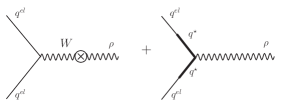
Figure 1: Two sources of the couplings between $\rho$ and quarks in the partial compositeness scenario. Left: from the mixing of $\rho$ with $W$ boson. Right: from the mixing of quarks with their composite partners.

II General Analysis

In light of completeness of the SM blocks, the presence of new heavy resonance states undoubtedly means the existence of beyond SM new particles and new interactions connecting them to the established fundamental elements. For concreteness, we consider a resonance $X$ decaying into two particles $A$ and $B$, where $A$ and $B$ are any species of (identical) particles within or beyond the SM, and the invariant mass $M_{AB}$ can be (partially) reconstructed at colliders. The amplitude $X\rightarrow AB$ can then be formally cast into the expression

$$\mathcal{M}^{S}_{X(AB)}=-\frac{\mathcal{M}^{\rm prod}_{X}\mathcal{M}_{X\rightarrow AB}}{M_{AB}^{2}-M_{X}^{2}+iM_{X}\Gamma_{X}}\,,$$ (1)

where $M_{X}$ and $\Gamma_{X}$ are, respectively, the mass and width of $X$, $\mathcal{M}^{\rm prod}_{X}$ and $\mathcal{M}_{X\rightarrow AB}$ the production and decay amplitudes. The propagator of $X$ has been explicitly shown, which is a crucial factor for the interference phenomena. In vicinity of the resonance, different prescriptions of the resonance structure lead to small discrepancies quantitatively, which becomes more significant when the width goes larger Englert:2015zra . As a viable approximation, we neglect such subtleness and work only in the standard Breit-Wigner formalism throughout this paper. In the mean time, the smooth background $\mathcal{M}_{\rm bkg}$ depends also on the invariant mass $M_{AB}$. In terms of the cross section, the signal goes like

$$\sigma^{S}_{X(AB)} = \int dM_{AB}\frac{S}{(M^{2}_{AB}-M_{X}^{2})^{2}+M_{X}^{2}\Gamma_{X}^{2}}$$ (2)

$$\sim \sigma^{S}_{X}{\rm BR}(X\rightarrow AB)\,,$$

where $S$ is some factor independent of the resonance propagator, and BR the branching ratio. On the other hand, the integrated interfering cross section reads

$$\sigma^{\rm int}_{X(AB)}=-2\int dM_{AB}\frac{(M^{2}_{AB}-M_{X}^{2})\Re+M_{X}\Gamma_{X}\Im}{(M^{2}_{AB}-M_{X}^{2})^{2}+M_{X}^{2}\Gamma_{X}^{2}}\ ,$$ (3)

where

$$\Re \equiv {\rm Re}(\mathcal{M}^{\rm prod}_{X}\mathcal{M}_{X\rightarrow AB}\mathcal{M}^{*}_{\rm bkg})\,,$$ (4)

$$\Im \equiv {\rm Im}(\mathcal{M}^{\rm prod}_{X}\mathcal{M}_{X\rightarrow AB}\mathcal{M}^{*}_{\rm bkg})$$ (5)

are, respectively, the real and imaginary contributions. We can see that in the on-shell region, the interference terms depend both on $\Re$ and $\Im$ as well as the width $\Gamma_{X}$. When the invariant mass is far away from the resonance, i.e. $|M^{2}_{AB}-M_{X}^{2}|\gg M_{X}\Gamma_{X}$, on the other hand, only the real part $\Re$ contribute and it goes like

$$\sim-2\frac{{\rm Re}(\mathcal{M}^{\rm prod}_{X}\mathcal{M}_{X\rightarrow AB}\mathcal{M}^{*}_{\rm bkg})}{M_{AB}^{2}-M_{X}^{2}}\,.$$ (6)

In a large variety of popular new physics models, the couplings of resonance $X$ to the decay products and/or the initial particles can take both positive and negative values. Consequently, the signal resonance can interfere with the continuum background constructively or destructively, depending on whether the signal and background amplitudes are additive or subtractive, as aforementioned. Given different signs of the couplings involved, say $\pm g_{XAB}$, the total cross sections $\sigma(pp\rightarrow X\rightarrow AB)$ are generally different, especially when the coupling is small such that the quadratic or higher order terms of $g_{XAB}$ in the cross section are not important Bian:2015zha .

As stated above, the signs of couplings could also change the line shape of $M_{AB}$. Specifically, the constructive interference tends to produce more events in the higher mass region $M_{AB}>M_{X}$ and, as a result, shift the peak to the upward direction to some extent, while the destructive interference distorts the resonance shape in a right opposite manner. To quantify the asymmetric effect, we define the parameter Lillie:2007ve

$$A_{i}\equiv\frac{\int{\rm d}M_{AB}\left[\frac{{\rm d}\sigma}{{\rm d}M_{AB}}-\left(\frac{{\rm d}\sigma}{{\rm d}M_{AB}}\right)_{\rm bkg}\right]\Theta(M_{AB}-M_{X})}{\int{\rm d}M_{AB}\left|\frac{{\rm d}\sigma}{{\rm d}M_{AB}}-\left(\frac{{\rm d}\sigma}{{\rm d}M_{AB}}\right)_{\rm bkg}\right|}\,,$$ (7)

where the $\Theta$-function is defined as

$$\Theta(x)\equiv\left\{\begin{array}[]{cc}-1,&x<0\\ 1,&x>0\end{array}\right.$$ (10)

which changes the sign when the resonance is crossed. The $A_{i}$ parameter could be either positive or negative depending on the signs of resonance couplings and vanishes for the pure background. The background contribution has been subtracted to determine if the interference is constructive or destructive. Note that with this definition, the sign of $A_{i}$ coincides with the relative sign between the signal and background amplitudes; in other words, $A_{i}>0\,(A_{i}<0)$ indicates the occurrence of constructive (destructive) interference.

Though the magnitudes of the numerator and denominator of $A_{i}$ depend on the binning of data in vicinity of the resonance, the sign of $A_{i}$ does not. One can extract the $A_{i}$ parameter from experimental data, and also obtain it from some underlying theories or models with different signs of couplings, say $\pm g_{XAB}$ for the $X$ resonance. By comparing the values of $A_{i}$ from experimental data and theoretical predictions, one can infer in a straightforward way which interference scheme is preferred, thus constraining the couplings and parameter space in some specific models.

III Limited statistics

We utilize a toy $W^{\prime}$ model to test the constructive/destructive signal-background interference in the ATLAS $WZ$ channel. It is expected that with the limited statistics and large background we can not have any significant hints of the signs of couplings.

Assuming simply the generation-universal coupling $g_{W^{\prime}ud}$ and the $W^{\prime}WZ$ coupling coefficient $g_{W^{\prime}WZ}$ in terms of the SM $WWZ$ interaction, the toy $W^{\prime}$ model can in some sense mimic the extra charged gauge boson in left-right symmetric models LRSM1 ; LRSM2 ; LRSM3 or the $\rho^{\pm}$ boson in composite Higgs models. To be more specific, we fix the mass $M_{W^{\prime}}=2$ TeV, the width $\Gamma_{W^{\prime}}=70$ GeV and $g_{W^{\prime}WZ}=+0.005$ Bian:2015ota ; Thamm2015 , then the constructive and destructive interference scenarios emerge as the coupling $g_{W^{\prime}ud}$ being, respectively, $\pm 0.15$. The signal process $pp\rightarrow W^{\prime}\rightarrow WZ$ interferes with the SM background $pp\rightarrow WZ$, with the $W^{\prime}$ boson naturally the origin of $\sim$ 2 TeV $WZ$ excess events.

We implement simple cuts on the fat $W$ and $Z$ jets: $p_{T}>540$ GeV and $|\eta|<2$. The smearing effect due to the finite detector resolution of the momenta of jets is taken into consideration, following the procedure in Aad:2015owa . Following Ref. ATLAS:combined , we assume the signal acceptance times efficiency factor of $\epsilon\simeq 0.07$. Given the benchmark values of input parameters for the $W^{\prime}$ models given above, we can fit roughly the ATLAS $WZ$ excess Pukhov:2004ca . Due to the limited statistics of current data, we use only the three bins from 1.85 to 2.15 TeV to calculate $A_{i}$, both for the constructive/destructive interference scenarios and the ATLAS $WZ$ data, which come out to be $\pm 0.11$ and $-0.52^{+1.52}_{-0.48}$. From these values we can see that the destructive interference is relatively preferred by the central value of $A_{i}$ from current data. However, as a result of the low statistics and large reducible non-interfering $JJ$ background, we can not distinguish clearly the two interference schemes. In the fit, we find that the jet smearing effect can moderately broaden the resonance and tend to slightly decrease the difference of $A_{i}$ for resonance couplings with different signs.

IV Prospects at large luminosity

It is promising that the constructive and destructive interference hypotheses can be more clearly differentiated at the higher energy, say LHC run II, with much more signal data. It is promising that with upcoming more data at 13 TeV LHC, we can have soon decisive conclusion on the resonance at 2 TeV. As an explicit example, we examine the signal background interference effect for the 2 TeV resonance at 14 TeV with a large luminosity.

To be concrete, we utilize the input parameters in the last section. All the four channels of leptonic, semileptonic, and hadronic decays are considered: $\ell\ell\ell^{\prime}\nu$, $\ell\ell q\bar{q}^{\prime}$, $\ell\nu q\bar{q}$ and $q\bar{q}q^{\prime}\bar{q}^{\prime\prime}$ with $\ell,\,\ell^{\prime}=e,\,\mu$. As the decay products are always highly boosted, it is common that some of the $q\bar{q}^{(\prime)}$ events appear to be large-$R$ jets. We simulate the signal process $pp\rightarrow W^{\prime}\rightarrow WZ$ and the dominate backgrounds in Table 1, and rescale simply the current 8 (or 13) TeV data to 14 TeV, assuming naïvely the event efficiencies being the same at the two energy scales. The signal acceptance times efficiency for the four distinct channels are from Fig. 1(a) of ATLAS:combined , where the branching fractions of $W/Z$ decays have been taken into consideration. The background simulations follow Refs atlas1 ; atlas2 ; atlas3 ; Aad:2015owa ; Khachatryan:2014gha , for which we implement only the basic event selection cuts. It should be aware that in the high mass region all these channels might suffer from large systematic and/or statistical uncertainties, depending on the future high energy data. In simulations we find that the hadronic channel is the most promising to confirm or exclude the 2 TeV resonance, due to the large branching ratio.

Table 1: Signals and dominate reducible/irreducible backgrounds in the $WZ$ final states at the 14 TeV LHC ATLAS:combined ; atlas1 ; atlas2 ; atlas3 ; Khachatryan:2014gha .

channel	backgrounds
$\ell\ell\ell^{\prime}\nu$	$WZ$
$\ell\ell q\bar{q}^{\prime}$	$Z+$jets
$\ell\nu q\bar{q}$	$W/Z+$jets
$q\bar{q}q^{\prime}\bar{q}^{\prime\prime}$	$jj$

As an explicit example of the interference effect, we show in Fig. 2 the invariant mass $M_{WZ}$ in the trileptonic and hadronic channels at the 14 TeV LHC. The simulated line shapes for the background and the constructive/destructive interfering resonances are shown, respectively, as dark, orange/blue lines, assuming a total luminosity of 3000 fb^-1. We reduce the rescaled $JJ$ background in the hadronic channel from the 8 TeV data by a factor of two, assuming for more events at LHC Run II more jet techniques are used and a more aggressive cut is made. For simplicity we implement only the simple cuts as did in atlas1 and Aad:2015owa . The quark jet smearing is performed as stated above, while for the charged leptons we assume naïvely the energy uncertainty $\Delta E/E\simeq 1\%$ Aad:2009wy . It is found that the lepton smearing have only tiny effect on the $M_{WZ}$ line shape and $A_{i}$. The expected local $A_{i}$ for the two channels are presented in Table 2.

For the “standard” scenarios Table 2, the central 17 bins (with a bin width of 50 GeV) around 2 TeV are used to calculate $A_{i}$. For the “optimal” scenarios, on the other hand, the central seven bins are removed in the calculation from the 17 bins, so only the $5+5=10$ bins with larger interference effect are used and we obtain the more aggressive predictions for the asymmetry factor while suffer from larger statistical uncertainties due to the reduced statistics. The uncertainties in the last column of Table 2 are the purely statistical one by simply counting the event numbers. It is expected that the constructive and destructive interference schemes can be differentiated at a reasonably large confidence level in both channels. In the trileptonic channel it could even be further improved to more than $5\sigma$ in the “optimal” scenario. Here we perform only rather naïve examinations of the prospects in the purely leptonic and hadronic channels, in the semileptonic channels we also expect a significant differentiation of the two interference schemes. When all these channels are combined together, the significance can even be further improved. Furthermore, more accurate estimations call for much more intricate simulations and analysis. Short in all, in light of the estimated $A_{i}$ and uncertainties in Table 2, given a huge amount of data at the current running LHC II and more refined experimental analysis, for instance the Boosted Decision Trees method Roe:2004na , we could probably reduce the statistical and systematic errors to a sufficiently low level such that we can measure the asymmetry factor $A_{i}$ precisely and pin down which interference hypothesis is the truth for the 2 TeV resonance, and thus constrain the signs of beyond SM couplings.

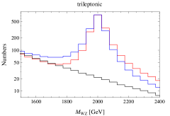
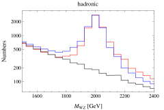
Figure 2: Invariant mass distribution of $M_{WZ}$ at the 14 TeV LHC: the dark, orange and blue lines indicate, respectively, the simulated background and resonances with constructive and destructive interference at the integrated luminosity of 3000 fb^-1.

Table 2: Expected local $A_{i}$ in the trileptonic and hadronic channels for the constructive/destructive interference schemes at the 14 TeV LHC, and their corresponding statistical uncertainties at the integrated luminosity of 3000 fb^-1.

$A_{i}$	scenario	constructive	destructive	uncertainty
trileptonic	standard	0.25	$-0.13$	0.09
	optimal	0.77	$-0.37$	0.18
hadronic	standard	0.20	$-0.10$	0.12
	optimal	0.79	$-0.33$	0.54

V Conclusions

Quantum interference is very common in the regime of elementary particle physics. In presence of some resonances on top of the continuum background, it is unavoidable that interference would occur between the signal and background. The shape of resonances depends both on the magnitudes of couplings involved and on the relative sign between the signal and background terms, i.e. whether the interference is constructive or destructive. In this work we point out how the resonance shape is affected and how to use the asymmetry parameter $A_{i}$ to differentiate the two distinct interference schemes.

Though a 2 TeV resonance is not favored by current 13 TeV data, the ATLAS diboson excesses are a viable illustrative candidate for the time being to test the implications of interference phenomena for future searches and studies of high mass resonances at LHC run II and the next-generation higher energy colliders. Implementing a toy $W^{\prime}$ model as a solution to the excess in $WZ$ channel, we find that the constructive and destructive interference schemes could be differentiated at a reasonably large confidence level in the trileptonic and hadronic $WZ$ decay channels (and also possible in the semileptonic channels), and further improved to more than $5\sigma$ in the “optimal” scenario for the trileptonic channel, as long as a huge statistics of signal events is achieved (a luminosity of 3000 fb^-1 assumed for the diboson events). Even if the 2 TeV excesses are excluded by upcoming data, the signal-background interference and resonance line shape are always useful to constrain the magnitudes and signs of beyond SM couplings and exclude large portions of parameter space in specific models.

References

- (1) M. R. Buckley, H. Murayama, W. Klemm and V. Rentala, Phys. Rev. D 78, 014028 (2008) [arXiv:0711.0364 [hep-ph]].
- (2) M. R. Buckley, B. Heinemann, W. Klemm and H. Murayama, Phys. Rev. D 77, 113017 (2008) [arXiv:0804.0476 [hep-ph]].
- (3) W. Y. Keung, I. Low and J. Shu, Phys. Rev. Lett. 101, 091802 (2008) [arXiv:0806.2864 [hep-ph]].
- (4) Q. H. Cao, C. B. Jackson, W. Y. Keung, I. Low and J. Shu, Phys. Rev. D 81, 015010 (2010) [arXiv:0911.3398 [hep-ph]].
- (5) H. Murayama, V. Rentala and J. Shu, arXiv:1401.3761 [hep-ph].
- (6) S. Jung, J. Song and Y. W. Yoon, arXiv:1505.00291 [hep-ph].
- (7) D. Choudhury, R. M. Godbole and P. Saha, JHEP 1201, 155 (2012) [arXiv:1111.1054 [hep-ph]].
- (8) D. Pappadopulo, A. Thamm, R. Torre and A. Wulzer, JHEP 1409, 060 (2014) [arXiv:1402.4431 [hep-ph]].
- (9) F. Caola and K. Melnikov, Phys. Rev. D 88, 054024 (2013) [arXiv:1307.4935 [hep-ph]].
- (10) V. Khachatryan et al. [CMS Collaboration], Phys. Lett. B 736, 64 (2014) [arXiv:1405.3455 [hep-ex]].
- (11) C. Englert and M. Spannowsky, Phys. Rev. D 90, 053003 (2014) [arXiv:1405.0285 [hep-ph]].
- (12) G. Cacciapaglia, A. Deandrea, G. Drieu La Rochelle and J. B. Flament, Phys. Rev. Lett. 113, no. 20, 201802 (2014) [arXiv:1406.1757 [hep-ph]].
- (13) C. Englert, I. Low and M. Spannowsky, Phys. Rev. D 91, no. 7, 074029 (2015) [arXiv:1502.04678 [hep-ph]].
- (14) N. Kauer and C. O Brien, Eur. Phys. J. C 75, 374 (2015) [arXiv:1502.04113 [hep-ph]].
- (15) N. Kauer and G. Passarino, JHEP 1208, 116 (2012) [arXiv:1206.4803 [hep-ph]].
- (16) D. A. Dicus and S. S. D. Willenbrock, Phys. Rev. D 37, 1801 (1988).
- (17) L. J. Dixon and M. S. Siu, Phys. Rev. Lett. 90, 252001 (2003) [hep-ph/0302233].
- (18) S. P. Martin, Phys. Rev. D 86, 073016 (2012) [arXiv:1208.1533 [hep-ph]].
- (19) L. J. Dixon and Y. Li, Phys. Rev. Lett. 111, 111802 (2013) [arXiv:1305.3854 [hep-ph]].
- (20) G. Z. Xu, G. Li, Y. J. Li, K. Y. Liu and Y. J. Zhang, arXiv:1505.06981 [hep-ph].
- (21) The ATLAS collaboration, ATLAS-CONF-2015-081; CMS Collaboration [CMS Collaboration], collisions at 13TeV,” CMS-PAS-EXO-15-004.
- (22) S. Jung, J. Song and Y. W. Yoon, arXiv:1601.00006 [hep-ph].
- (23) G. Aad et al. [ATLAS Collaboration], arXiv:1506.00962 [hep-ex].
- (24) L. Bian, D. Liu and J. Shu, arXiv:1507.06018 [hep-ph].
- (25) A. Thamm, R. Torre and A. Wulzer, arXiv:1506.08688 [hep-ph].
- (26) H. S. Fukano, M. Kurachi, S. Matsuzaki, K. Terashi and K. Yamawaki, arXiv:1506.03751 [hep-ph].
- (27) J. Hisano, N. Nagata and Y. Omura, arXiv:1506.03931 [hep-ph].
- (28) D. B. Franzosi, M. T. Frandsen and F. Sannino, arXiv:1506.04392 [hep-ph].
- (29) K. Cheung, W. Y. Keung, P. Y. Tseng and T. C. Yuan, arXiv:1506.06064 [hep-ph].
- (30) B. A. Dobrescu and Z. Liu, arXiv:1506.06736 [hep-ph].
- (31) J. A. Aguilar-Saavedra, arXiv:1506.06739 [hep-ph].
- (32) A. Alves, A. Berlin, S. Profumo and F. S. Queiroz, arXiv:1506.06767 [hep-ph].
- (33) Y. Gao, T. Ghosh, K. Sinha and J. H. Yu, arXiv:1506.07511 [hep-ph].
- (34) J. Brehmer, J. Hewett, J. Kopp, T. Rizzo and J. Tattersall, arXiv:1507.00013 [hep-ph].
- (35) Q. H. Cao, B. Yan and D. M. Zhang, arXiv:1507.00268 [hep-ph].
- (36) G. Cacciapaglia and M. T. Frandsen, arXiv:1507.00900 [hep-ph].
- (37) T. Abe, R. Nagai, S. Okawa and M. Tanabashi, arXiv:1507.01185 [hep-ph].
- (38) J. Heeck and S. Patra, arXiv:1507.01584 [hep-ph].
- (39) B. C. Allanach, B. Gripaios and D. Sutherland, arXiv:1507.01638 [hep-ph].
- (40) T. Abe, T. Kitahara and M. M. Nojiri, arXiv:1507.01681 [hep-ph].
- (41) A. Carmona, A. Delgado, M. Quiros and J. Santiago, arXiv:1507.01914 [hep-ph].
- (42) B. A. Dobrescu and Z. Liu, arXiv:1507.01923 [hep-ph].
- (43) C. W. Chiang, H. Fukuda, K. Harigaya, M. Ibe and T. T. Yanagida, arXiv:1507.02483 [hep-ph].
- (44) G. Cacciapaglia, A. Deandrea and M. Hashimoto, arXiv:1507.03098 [hep-ph].
- (45) H. S. Fukano, S. Matsuzaki and K. Yamawaki, arXiv:1507.03428 [hep-ph].
- (46) V. Sanz, arXiv:1507.03553 [hep-ph].
- (47) C. H. Chen and T. Nomura, arXiv:1507.04431 [hep-ph].
- (48) M. E. Krauss and W. Porod, arXiv:1507.04349 [hep-ph].
- (49) Y. Omura, K. Tobe and K. Tsumura, arXiv:1507.05028 [hep-ph].
- (50) W. Chao, arXiv:1507.05310 [hep-ph].
- (51) L. A. Anchordoqui, I. Antoniadis, H. Goldberg, X. Huang, D. Lust and T. R. Taylor, arXiv:1507.05299 [hep-ph].
- (52) D. Kim, K. Kong, H. M. Lee and S. C. Park, arXiv:1507.06312 [hep-ph].
- (53) H. Fritzsch, arXiv:1507.06499 [hep-ph].
- (54) K. Lane and L. Prichett, arXiv:1507.07102 [hep-ph].
- (55) A. E. Faraggi and M. Guzzi, arXiv:1507.07406 [hep-ph].
- (56) M. Low, A. Tesi and L. T. Wang, arXiv:1507.07557 [hep-ph].
- (57) S. P. Liew and S. Shirai, arXiv:1507.08273 [hep-ph].
- (58) H. Terazawa and M. Yasue, arXiv:1508.00172 [hep-ph].
- (59) P. Arnan, D. Espriu and F. Mescia, arXiv:1508.00174 [hep-ph].
- (60) C. Niehoff, P. Stangl and D. M. Straub, arXiv:1508.00569 [hep-ph].
- (61) P. S. B. Dev and R. N. Mohapatra, arXiv:1508.02277 [hep-ph].
- (62) A. Dobado, F. K. Guo and F. J. Llanes-Estrada, arXiv:1508.03544 [hep-ph].
- (63) P. Coloma, B. A. Dobrescu and J. Lopez-Pavon, arXiv:1508.04129 [hep-ph].
- (64) S. Fichet and G. von Gersdorff, arXiv:1508.04814 [hep-ph].
- (65) C. Petersson and R. Torre, arXiv:1508.05632 [hep-ph].
- (66) F. F. Deppisch, L. Graf, S. Kulkarni, S. Patra, W. Rodejohann, N. Sahu and U. Sarkar, arXiv:1508.05940 [hep-ph].
- (67) D. Gonçalves, F. Krauss and M. Spannowsky, Phys. Rev. D 92, no. 5, 053010 (2015) [arXiv:1508.04162 [hep-ph]].
- (68) D. Marzocca, M. Serone and J. Shu, JHEP 1208, 013 (2012) [arXiv:1205.0770 [hep-ph]].
- (69) L. Bian, J. Shu and Y. Zhang, arXiv:1507.02238 [hep-ph].
- (70) B. Lillie, J. Shu and T. M. P. Tait, Phys. Rev. D 76, 115016 (2007) [arXiv:0706.3960 [hep-ph]].
- (71) J. C. Pati and A. Salam, Phys. Rev. D 10, 275 (1974) [Phys. Rev. D 11, 703 (1975)].
- (72) R. N. Mohapatra and J. C. Pati, Phys. Rev. D 11, 566 (1975).
- (73) G. Senjanovic and R. N. Mohapatra, Phys. Rev. D 12, 1502 (1975).
- (74) ATLAS Collaboration, ATLAS-CONF-2015-045.
- (75) A. Pukhov, hep-ph/0412191.
- (76) G. Aad et al. [ATLAS Collaboration], Phys. Lett. B 737, 223 (2014) [arXiv:1406.4456 [hep-ex]].
- (77) G. Aad et al. [ATLAS Collaboration], Eur. Phys. J. C 75, no. 2, 69 (2015) [arXiv:1409.6190 [hep-ex]].
- (78) G. Aad et al. [ATLAS Collaboration], Eur. Phys. J. C 75, no. 5, 209 (2015) [Eur. Phys. J. C 75, 370 (2015)] [arXiv:1503.04677 [hep-ex]].
- (79) V. Khachatryan et al. [CMS Collaboration], JHEP 1408, 174 (2014) [arXiv:1405.3447 [hep-ex]].
- (80) G. Aad et al. [ATLAS Collaboration], arXiv:0901.0512 [hep-ex].
- (81) B. P. Roe, H. J. Yang, J. Zhu, Y. Liu, I. Stancu and G. McGregor, Nucl. Instrum. Meth. A 543, no. 2-3, 577 (2005) [physics/0408124].