Robust regression estimation and inference in the presence of cellwise and casewise contamination

Abstract

Cellwise outliers are likely to occur together with casewise outliers in modern datasets of relatively large dimension. Recent work has shown that traditional robust regression methods may fail when applied to such datasets. We propose a new robust regression procedure to deal with casewise and cellwise outliers. The proposed method, called three-step regression, proceeds as follows: first, it uses a consistent univariate filter, that is, a procedure that flags and eliminates extreme cellwise outliers; second, it applies a robust estimator of multivariate location and scatter to the filtered data to down-weight casewise outliers; third, it computes robust regression coefficients from the estimates obtained in the second step. The three-step estimator is consistent and asymptotically normal at the central model under some assumptions on the tails of the distributions of the continuous covariates. The estimator is extended to handle both continuous and dummy covariates using an iterative algorithm. Extensive simulation results show that the three-step estimator is resilient to cellwise outliers. It also performs well under casewise contamination when compared to traditional high breakdown point estimators.

1 Introduction

The vast majority of procedures for robust linear regression are based on the classical Tukey–Huber contamination model (THCM) in which a relatively small fraction of cases may be contaminated. High breakdown point affine equivariant estimators such as least trimmed squares (Rousseeuw, 1984), S-regression (Rousseeuw and Yohai, 1984) and MM-regression (Yohai, 1985) proceed by down-weighting outlying cases, which makes sense and works well in practice, under THCM. However, in some applications, the contamination mechanism may be different in that random cells in a data table (with rows as cases and columns as variables) are independently contaminated. In this paradigm, a small fraction of random cellwise outliers could propagate to a relatively large fraction of cases, breaking down classical high breakdown point affine equivariant estimators (see Alqallaf et al., 2009). Since cellwise and casewise outliers may co-exist in some applications, our goal in this paper is to develop a method for robust regression estimation and inference that can deal with both cellwise and casewise outliers.

There is a vast literature on robust regression for casewise outliers, but only a scant literature for cellwise outliers and none for both types of outliers in the regression context. Recently, Öllerer et al. (2015) combined the ideas of coordinate descent algorithm (called the shooting algorithm in Fu, 1998) and simple S-regression (Rousseeuw and Yohai, 1984) to propose an estimator called the shooting S. The shooting S-estimator assigns individual weight to each cell in the data table to handle cellwise outliers in the regression context. The shooting S-estimator is robust against cellwise outliers and vertical response outliers.

In this paper, we propose a three-step regression estimator which combines the ideas of filtering cellwise outliers and robust regression via covariance matrix estimate (Maronna and Morgenthaler, 1986; Croux et al., 2003), namely 3S-regression estimator. By filtering, here we mean detecting outliers and replacing them by missing values as in Agostinelli et al. (2015). Our estimator proceeds as follows: first, it uses a univariate filter to detect and eliminate extreme cellwise outliers in order to control the effect of outliers propagation; second, it applies a robust estimator of multivariate location and scatter to the filtered data to down-weight casewise outliers; third, it computes robust regression coefficients from the estimates obtained in the second step. With the choice of a filter that has simultaneous good sensitivity (is capable of filtering outliers) and good specificity (can preserve all or most of the clean data), the resulting estimator can be resilient to both cellwise and casewise outliers; furthermore, it attains consistency and asymptotic normality for clean data. In this regards, we propose a filter that is consistent under some assumptions on the tails of the covariates distributions. By consistent filter, we mean a filter that asymptotically can preserve all the data when they are clean.

The rest of the paper is organized as follows. In Section 2, we introduce a family of consistent filters. In Section 3, we introduce 3S-regression. In Section 4, we show some asymptotic properties of 3S-regression. In Section 5, we evaluate the performance of 3S-regression in an extensive simulation study. In Section 6, we analyze a real data set with cellwise and casewise outliers. In Section 7, we conclude with some remarks. We also provide a document referred to as “supplementary material”, which contains all the proofs, additional simulation results, and other related material.

2 Consistent filter

Filtering is a method for pre-processing data in order to control the effect of potential cellwise outliers. In this paper, we pre-process the data by flagging outliers and replacing them by missing values, NAs. This method of filtering has recently been used for robust estimation of multivariate location and scatter (Danilov, 2010; Agostinelli et al., 2015) and for clustering (Farcomeni, 2014a, b). Also, Farcomeni (2015) proposed a procedure to determine a data-driven choice for the number of filtered cells to increase the efficiency of the estimator.

Consistent filters are ones that do not filter good data points asymptotically. Gervini and Yohai (2002) introduced a consistent filter for normal residuals in regression estimation to achieve a fully-efficient robust regression estimator. Consistent filters are desirable because their good asymptotic properties are shared by the following-up estimation procedure. In this paper, we introduce a new family of consistent filters for univariate data.

Consider a random variable $X$ with a continuous distribution function $G(x)$. We define the scaled upper and lower tail distributions of $G(x)$ as follows:

$$F^{u}(t) =P_{G}\left(\frac{X-\eta^{u}}{\text{med}(X-\eta^{u}|X>\eta^{u})}\leq t|X>\eta^{u}\right)\quad\text{and}$$ (1)

$$F^{l}(t) =P_{G}\left(\frac{\eta^{l}-X}{\text{med}(\eta^{l}-X|X<\eta^{l})}\leq t|X<\eta^{l}\right).$$

Here, med stands for median, $\eta^{u}=G^{-1}(1-\alpha)$, $\eta^{l}=G^{-1}(\alpha)$, and $0<\alpha<0.5$. We use $\alpha=0.20$, but other choices could be considered. To simplify the notation, we set $s^{u}=\text{med}(X-\eta^{u}|X>\eta^{u})$ and $s^{l}=\text{med}(\eta^{l}-X|X<\eta^{l})$. Alternatively, a combined tails approach could be used for symmetric distributions as in Gervini and Yohai (2002).

Let $\{X_{1},\dots,X_{n}\}$ be a random sample from $G$, and let $X_{(1)}<X_{(2)}<\dots<X_{(n)}$ be the corresponding order statistics. Consistent estimators for $(\eta^{u},s^{u},\eta^{l},s^{l})$ are given by

$$\hat{\eta}^{u}_{n} =\hat{G}^{-1}_{n}(1-\alpha),\quad\hat{s}^{u}_{n}=\text{med}(\{X_{i}-\hat{\eta}^{u}_{n}|X_{i}>\hat{\eta}^{u}_{n}\}),$$

$$\hat{\eta}^{l}_{n} =\hat{G}^{-1}_{n}(\alpha),\quad\hat{s}^{l}_{n}=\text{med}(\{\hat{\eta}^{l}_{n}-X_{i}|X_{i}<\hat{\eta}^{l}_{n}\}),$$

where $\hat{G}_{n}^{-1}(a)=X_{(\lceil na\rceil)}$, $0<a<1$, is the empirical quantile and $\text{med}(\{Y_{1},\dots,Y_{m}\})=Y_{(\lceil m/2\rceil)}$ is the sample median (see Lemma 1.1 in the supplementary material for a proof of the consistency for $\hat{s}^{u}_{n}$ and $\hat{s}^{l}_{n}$). The empirical distribution functions for the scaled upper and lower tails in (1) are now given by

$$\hat{F}^{u}_{n}(t) =\frac{\sum_{i=1}^{n}I(0<(X_{i}-\hat{\eta}^{u}_{n})/\hat{s}^{u}_{n}\leq t)}{\sum_{i=1}^{n}I(X_{i}>\hat{\eta}^{u}_{n})}\quad\text{and}$$

$$\hat{F}^{l}_{n}(t) =\frac{\sum_{i=1}^{n}I(0<(\hat{\eta}^{l}_{n}-X_{i})/\hat{s}^{l}_{n}\leq t)}{\sum_{i=1}^{n}I(X_{i}<\hat{\eta}^{l}_{n})}.$$

Upper and lower tails outliers can be flagged by comparing the empirical distribution functions for the scaled tails with their expected distributions. We assume that aside from contamination, $F^{u}$ and $F^{l}$ decay exponentially fast or faster. Let $\{a\}^{+}=\max(0,a)$ denote the positive part of $a$. Then, we define the proportions of flagged upper and lower tails outliers by

$$\hat{d}^{u}_{n} =\sup_{t\geq t_{0}}\left\{F_{0}(t)-\hat{F}^{u}_{n}(t)\right\}^{+}\quad\text{and}\quad\hat{d}^{l}_{n} =\sup_{t\geq t_{0}}\left\{F_{0}(t)-\hat{F}^{l}_{n}(t)\right\}^{+},$$

where $F_{0}(t)=1-\exp(-\log(2)t)$ and $t_{0}=1/\log(2)$. When $X-\eta^{u}|X>\eta^{u}$ is exponentially distributed with a rate of $\lambda^{u}>0$, the standardized tail $(X-\eta^{u})/s^{u}|X>\eta^{u}$ have exponential distribution with a rate of $\log(2)$, leading to our choice of $F_{0}(t)$ and $t_{0}$. Finally, we filter $\hat{d}^{u}_{n}\times 100\%$ of the most extreme points in the upper tail $\{X_{i}|X_{i}>\hat{\eta}^{u}_{n}\}$, and filter $\hat{d}^{l}_{n}\times 100\%$ of the most extreme points in the lower tail $\{X_{i}|X_{i}<\hat{\eta}^{l}_{n}\}$. Equivalently, setting

$$\hat{t}^{u}_{n} =\min\left\{t:\hat{F}^{u}_{n}(t)\geq 1-\hat{d}^{u}_{n}\right\}\quad\text{and}\quad\hat{t}^{l}_{n} =\min\left\{t:\hat{F}^{l}_{n}(t)\geq 1-\hat{d}^{l}_{n}\right\},$$

we filter $X_{i}$’s with $X_{i}<\hat{\eta}^{l}_{n}-\hat{s}^{l}_{n}\hat{t}^{l}_{n}$ or $X_{i}>\hat{\eta}^{u}_{n}+\hat{s}^{u}_{n}\hat{t}^{u}_{n}$.

We tried several heavy tail models for $F_{0}(t)$ including Pareto distributions with different tail indexes, and we found that the chosen exponential model strikes a good balance between the robustness and consistency of the filtering procedure.

Theorem 2.1 (proved in the supplementary material) below shows that our filter is consistent under the following assumption on the tails of $G(x)$.

Assumption 2.1.

$G(x)$ is continuous, and $F^{u}(t)$ and $F^{l}(t)$ satisfy the following:

$$F_{0}(t)-F^{u}(t)\leq 0,\quad t\geq t_{0}\quad\text{and}\quad F_{0}(t)-F^{l}(t)\leq 0,\quad t\geq t_{0}.$$

Theorem 2.1.

Suppose that Assumption 2.1 holds for $G(x)$. Then, $\hat{d}^{u}_{n}\to 0$ a.s. and $\hat{d}^{l}_{n}\to 0$ a.s.

In practice, the distributions $F^{u}(t)$ and $F^{l}(t)$ are unknown. To allow for some flexibility, Assumption 2.1 does not completely specify $F^{u}(t)$ and $F^{l}(t)$, but it only requires that their upper tails are as heavy as or lighter than the upper tail of $F_{0}(t)$.

3 Three-step regression

3.1 The estimator

Consider the model

$$Y_{i}=\alpha+\boldsymbol{X}_{i}^{t}\boldsymbol{\beta}+\varepsilon_{i}$$ (2)

for $i=1,\dots,n$, where the error terms $\varepsilon_{i}$ are i.i.d. and independent of the covariates $\boldsymbol{X}_{i}=(X_{i1},\dots,X_{ip})^{t}$. The least squares (LS) estimates $(\hat{\alpha}_{LS},\hat{\boldsymbol{\beta}}^{t}_{LS})$ are defined as the minimizers of the sum squares of residuals,

$$(\hat{\alpha}_{LS},\hat{\boldsymbol{\beta}}^{t}_{LS})=\underset{(\alpha,\boldsymbol{\beta}^{t})\in\mathbb{R}^{(p+1)}}{\arg\min}\sum_{i=1}^{n}(Y_{i}-\alpha-\boldsymbol{X}_{i}^{t}\boldsymbol{\beta})^{2}.$$

The solution to this problem is explicit:

$$\hat{\boldsymbol{\beta}}_{LS} =\hat{\boldsymbol{\Sigma}}_{xx}^{-1}\hat{\boldsymbol{\Sigma}}_{xy},$$ (3)

$$\hat{\alpha}_{LS} =\hat{\mu}_{y}-\hat{\boldsymbol{\mu}}_{x}^{t}\hat{\boldsymbol{\beta}}_{LS}.$$

Here, $\hat{\boldsymbol{\Sigma}}_{xx},\hat{\boldsymbol{\Sigma}}_{xy},\hat{\mu}_{y}$, and $\hat{\boldsymbol{\mu}}_{x}$ are the components of the empirical covariance matrix and mean:

$$\hat{\boldsymbol{\Sigma}}=\left(\begin{array}[]{cc}\hat{\boldsymbol{\Sigma}}_{xx}&\hat{\boldsymbol{\Sigma}}_{xy}\\ \hat{\boldsymbol{\Sigma}}_{yx}&\hat{\Sigma}_{yy}\end{array}\right)\quad\text{and}\quad\hat{\boldsymbol{\mu}}=\left(\begin{array}[]{c}\hat{\boldsymbol{\mu}}_{x}\\ \hat{\mu}_{y}\end{array}\right)$$ (4)

for the joint data $\{\boldsymbol{Z}_{1},\dots,\boldsymbol{Z}_{n}\}$ with $\boldsymbol{Z}_{i}=(\boldsymbol{X}_{i}^{t},Y_{i})^{t}$.

Several authors (see Maronna and Morgenthaler, 1986; Croux et al., 2003) proposed to achieve robust regression and inference for casewise outliers by robustifying the components in (3). Croux et al. (2003) replaced the empirical covariance matrix and mean by the multivariate S-estimator (Davies, 1987). We will refer to this approach as two-step regression (2S-regression). Croux et al. (2003) have shown that under mild assumptions (including symmetry of $\varepsilon_{i}$ and independence of $\varepsilon_{i}$ and $\boldsymbol{X}_{i}$) 2S-regression is Fisher consistent and asymptotically normal even if the S-estimators of multivariate location and scatter themselves are not consistent. Furthermore, 2S-regression is resilient to all kinds of outliers, that is, vertical outliers, bad leverage points, and good leverage points. Note that down-weighting good leverage points could lead to some efficiency loss, but it may also prevent the underestimation of the variance of the estimator, which could be problematic for inferential purposes (see for example, Ruppert and Simpson, 1990).

To deal with casewise and cellwise outliers, we propose to use a generalized S-estimator that uses the consistent filter described in Section 2. The estimator is similar to that in Agostinelli et al. (2015), but with the filter which is consistent for a broader range of distributions. This generality is needed in the regression setting. Our proposed globally robust regression estimator, called 3S-regression, is given by:

$$\hat{\boldsymbol{\beta}}_{3S} =\hat{\boldsymbol{S}}_{xx}^{-1}\hat{\boldsymbol{S}}_{xy}$$ (5)

$$\hat{\alpha}_{3S} =\hat{m}_{y}-\hat{\boldsymbol{m}}_{x}^{t}\hat{\boldsymbol{\beta}}_{3S}.$$

Here, $(\hat{\boldsymbol{m}},\hat{\boldsymbol{S}})$ is a generalized S-estimator computed as follows:

1. Filter extreme cellwise outliers to prevent cellwise contaminated cases from having large robust Mahalanobis distances in Step 2, and

2. Down-weight casewise outliers by applying generalized S-estimator (GSE) for multivariate location and scatter (Danilov et al., 2012) to the filtered data from Step 1. The GSE is a generalization of the S-estimator for incomplete data that are missing completely at random (MCAR). Since the independent contamination model (ICM) assumes that cells are outlying completely at random, the MCAR assumption is fulfilled if the ICM model holds.

More precisely, consider a set of covariates $\{\boldsymbol{X}_{1},\dots,\boldsymbol{X}_{n}\}$. We perform univariate filtering as described in Section 2 on each variable, $\{X_{1j},\dots,X_{nj}\}$, $j=1,\dots,p$. Let $\{\boldsymbol{U}_{1},\dots,\boldsymbol{U}_{n}\}$ be the resulting auxiliary vectors of zeros and ones with zeros indicating the filtered entry in $\boldsymbol{X}_{i}$. More precisely, $\boldsymbol{U}_{i}=(U_{i1},\dots,U_{ip})^{t}$, where

$$U_{ij}=I(\hat{\eta}^{l}_{j,n}-\hat{s}^{l}_{j,n}\hat{t}^{l}_{j,n}\leq X_{i}\leq\hat{\eta}^{u}_{j,n}+\hat{s}^{u}_{j,n}\hat{t}^{u}_{j,n}).$$

The goal of the filter is to prevent propagation of cellwise outliers. If the fraction of cases with at least one flagged cell is very small (below $1\%$, say) then propagation of cellwise outliers is not an issue and the filter can be safely turned off. The procedure that turns the filter off when the fraction of affected cases is below a given small threshold, $\xi$, is considerably simpler to analyze from the asymptotic point of view. Moreover, it retains all the robustness properties derived from the filter. Let $n_{0}=\#\{1\leq i\leq n:\boldsymbol{U}_{i}=\boldsymbol{1}\}$ be the number of complete observations after filtering. We set

$$\boldsymbol{U}^{*}_{i}=\boldsymbol{1}I\left(\frac{n-n_{0}}{n}\leq\xi\right)+\boldsymbol{U}_{i}I\left(\frac{n-n_{0}}{n}>\xi\right),\quad i=1,\dots,n,$$ (6)

with $\xi$ equal to some small threshold. In this paper we use $\xi=0.01$.

Finally, let $\mathbb{Z}=(\boldsymbol{Z}_{1},\dots,\boldsymbol{Z}_{n})^{t}$ and $\mathbb{U}=((\boldsymbol{U}_{1}^{*},\dots,\boldsymbol{U}_{n}^{*})^{t},\boldsymbol{1})$. The generalized S-estimator can now be defined as

$$\hat{\boldsymbol{m}} =\hat{\boldsymbol{m}}_{GS}(\mathbb{Z},\mathbb{U}),$$ (7)

$$\hat{\boldsymbol{S}} =\hat{\boldsymbol{S}}_{GS}(\mathbb{Z},\mathbb{U}),$$

where $\hat{\boldsymbol{m}}_{GS}$ and $\hat{\boldsymbol{S}}_{GS}$ are robust multivariate location and scatter generalized S-estimator for incomplete data, $(\mathbb{Z},\mathbb{U})$, with Tukey’s bisquare rho function $\rho_{B}(t)=\min(1,1-(1-t)^{3})$ and 50% breakdown point (see Danilov et al., 2012, for full definition). Note that when $\mathbb{U}=(\boldsymbol{1},\dots,\boldsymbol{1})$ (i.e., when the input data is complete), the generalized S-estimator reduces to S-estimator (Danilov et al., 2012).

3.2 Models with continuous and dummy covariates

For models with continuous and dummy covariates, the direct computation of 3S-regression is likely to fail because the sub-sampling algorithm (needed to compute the generalized S-estimator) is likely to yield collinear subsamples. In this case, we endow 3S-regression with an iterative algorithm similar to that in Maronna and Yohai (2000) to deal with continuous and dummy covariates.

Consider now the following model:

$$Y_{i}=\alpha+\boldsymbol{X}_{i}^{t}\boldsymbol{\beta}_{x}+\boldsymbol{D}_{i}^{t}\boldsymbol{\beta}_{d}+\varepsilon_{i}$$ (8)

for $i=1,\dots,n$ where $\boldsymbol{X}_{i}=(X_{i1},\dots,X_{ip_{x}})^{t}$ is a $p_{x}$ dimensional vector of continuous covariates and $\boldsymbol{D}_{i}=(D_{i1},\dots,D_{ip_{d}})^{t}$ is a $p_{d}$ dimensional vector of dummy covariates. Set $\mathbb{X}=(\boldsymbol{X}_{1},\dots,\boldsymbol{X}_{n})^{t}$, $\mathbb{D}=(\boldsymbol{D}_{1},\dots,\boldsymbol{D}_{n})^{t}$, and $\boldsymbol{Y}=(Y_{1},\dots,Y_{n})^{t}$. We assume that the columns in $\mathbb{X}$ and $\mathbb{D}$ are linearly independent.

We modify the alternating M- and S-regression approach proposed by Maronna and Yohai (2000). Our algorithm uses 3S-regression to estimate the coefficients of the continuous covariates and regression M-estimators with Huber’s rho function $\rho_{H}(t)=\min(1,t^{2}/2)$ (Huber and Ronchetti, 2009) to estimate the coefficients of the dummy covariates. More specifically, the algorithm works as follows:

$$(\hat{\alpha}^{(k)},\hat{\boldsymbol{\beta}}_{x}^{(k)}) =g(\mathbb{X},\boldsymbol{Y}-\mathbb{D}\hat{\boldsymbol{\beta}}_{d}^{(k-1)}),$$ (9)

$$\hat{\boldsymbol{\beta}}_{d}^{(k)} =M(\mathbb{D},\boldsymbol{Y}-\hat{\alpha}^{(k)}-\hat{\mathbb{X}}\hat{\boldsymbol{\beta}}_{x}^{(k)}),\quad\text{for}\quad k=1,\dots,K,$$

where $g(\mathbb{X},\boldsymbol{Y})$ denotes the operation of 3S-regression for a response vector $(\boldsymbol{Y},\mathbb{X})$ as defined in (5) and $M(\mathbb{D},\boldsymbol{Y})$ denotes the operation of regression $M$-estimator with no intercept for $(\boldsymbol{Y},\mathbb{D})$. We let $\hat{\mathbb{X}}$ be the imputed $\mathbb{X}$ with the filtered entries imputed by the best linear predictor using $\hat{\boldsymbol{m}}^{(k)}$ and $\hat{\boldsymbol{S}}^{(k)}$, the generalized S-estimates at the $k$-th iteration as defined in (7). We use $\hat{\mathbb{X}}$ instead of $\mathbb{X}$ to control the effect of propagation of cellwise outliers.

As in Maronna and Yohai (2000), to calculate the initial estimates, $(\hat{\alpha}^{(0)},\hat{\boldsymbol{\beta}}_{x}^{(0)},\hat{\boldsymbol{\beta}}_{d}^{(0)})$, we first remove the effect of $\boldsymbol{D}_{i}$ from the continuous covariates and the response variable. Let

$$\overline{\boldsymbol{Y}}=\boldsymbol{Y}-\mathbb{D}\boldsymbol{t}\quad\text{and}\quad\overline{\mathbb{X}}=\mathbb{X}-\mathbb{D}\mathbb{T},$$

where $\boldsymbol{t}=M(\mathbb{D},\boldsymbol{Y})$ and $\mathbb{T}$ is a $p_{d}\times p_{x}$-matrix with the $j$-th column as $\boldsymbol{T}_{j}=M(\mathbb{D},(X_{1j},\dots,X_{nj})^{t})$. Now, the initial estimates are defined by

$$(\hat{\alpha}^{(0)},\hat{\boldsymbol{\beta}}_{x}^{(0)t}) =g(\overline{\mathbb{X}},\overline{\boldsymbol{Y}}),$$

$$\hat{\boldsymbol{\beta}}_{d}^{(0)} =M(\mathbb{D},\boldsymbol{Y}-\hat{\alpha}^{(0)}-\hat{\mathbb{X}}\hat{\boldsymbol{\beta}}_{x}^{(0)}).$$

Finally, the procedure in (9) is iterated until convergence or until it reaches a maximum of $K=20$ iterations. We choose $K=20$ because our simulation has shown that the procedure usually converges for $K<20$, provided good initial estimates are used.

4 Asymptotic properties of three-step regression

Theorem 4.1 (proved in the supplementary material) establishes the equivalence between 3S-regression and 2S-regression (Croux et al., 2003) for the case of continuous covariates. Let $(\hat{\alpha}_{3S},\hat{\boldsymbol{\beta}}_{3S}^{t})$ be the 3S-regression estimate and $(\hat{\alpha}_{2S},\hat{\boldsymbol{\beta}}_{2S}^{t})$ be the 2S-regression estimate based on the sample $\{\boldsymbol{Z}_{1},\dots,\boldsymbol{Z}_{n}\}$, where $\boldsymbol{Z}_{i}=(\boldsymbol{X}^{t}_{i},Y_{i})$. Let $G(\boldsymbol{x})$ and $G_{j}(x)$ be the distribution functions for $\boldsymbol{X}_{i}$ for $X_{ij}$ respectively.

Theorem 4.1.

Suppose that Assumption 2.1 holds for each $G_{j}$, $j=1,\dots,p$. Then, with probability one, for sufficiently large $n$, $\hat{\alpha}_{3S}=\hat{\alpha}_{2S}$ and $\hat{\boldsymbol{\beta}}_{3S}=\hat{\boldsymbol{\beta}}_{2S}$.

Since 3S-regression becomes 2S-regression for sufficiently large $n$, 3S-regression inherits the established asymptotic properties of 2S-regression. Corollary 4.2 states the strong consistency and asymptotic normality of 3S-regression. The corollary requires the following regularity assumptions that are needed for deriving the consistency and asymptotic normality of 2S-regression (see Croux et al., 2003).

Assumption 4.1.

Let $F_{\varepsilon}$ be the distribution of the error term $\varepsilon_{i}$ in (2). The distribution $F_{\varepsilon}$ has a positive, symmetric and unimodal density $f_{\varepsilon}$.

Assumption 4.2.

For all $\boldsymbol{v}\in\mathbb{R}^{p}$ and $\delta\in\mathbb{R}$, $P_{G}(\boldsymbol{X}_{i}^{t}\boldsymbol{v}=\delta)<1/2$.

Corollary 4.2.

Suppose that Assumption 2.1 holds for each $G_{j}$, $j=1,\dots,p$, and Assumption 4.1–4.2 hold. Denote $\hat{\boldsymbol{\theta}}_{3S}=(\hat{\alpha}_{3S},\hat{\boldsymbol{\beta}}_{3S}^{t})^{t}$ and $\boldsymbol{\theta}=(\alpha,\boldsymbol{\beta}^{t})^{t}$. Then,

1. $\hat{\theta}_{3S}\to\theta$ a.s..

2. Let $H$ be the distribution of $(\boldsymbol{X}^{t},Y)$ and let $(\boldsymbol{m}_{H},\boldsymbol{S}_{H})$ be the S-estimator functional (see Lopuhaä, 1989). We use the same partition outlined in (4) for $(\boldsymbol{m}_{H},\boldsymbol{S}_{H})$. Set $\tilde{\boldsymbol{X}}=(1,\boldsymbol{X}^{t})^{t}$. Then,

   $$\sqrt{n}(\hat{\boldsymbol{\theta}}_{3S}-\boldsymbol{\theta})\to_{d}N(\boldsymbol{0},ASV(H)),$$

   where

   $$ASV(H)=C(H)^{-1}D(H)C(H)^{-1},$$

   and where

   $$C(H) =E_{H}\left\{w(d_{H}(\boldsymbol{Z}))\tilde{\boldsymbol{X}}\tilde{\boldsymbol{X}}^{t}\right\}+\frac{2}{\sigma^{2}_{\varepsilon}(H)}E_{H}\left\{w^{\prime}(d_{H}(\boldsymbol{Z}))(Y-\tilde{\boldsymbol{X}}^{t}\boldsymbol{\theta})^{2}\tilde{\boldsymbol{X}}\tilde{\boldsymbol{X}}^{t}\right\},$$

   $$D(H) =E_{H}\left\{w^{2}(d_{H}(\boldsymbol{Z}))(Y-\tilde{\boldsymbol{X}}^{t}\boldsymbol{\theta})^{2}\tilde{\boldsymbol{X}}\tilde{\boldsymbol{X}}^{t}\right\},$$

   $$\sigma_{\varepsilon}(H) =\sqrt{S_{H,yy}-\boldsymbol{\beta}^{t}\boldsymbol{S}_{H,xx}\boldsymbol{\beta}},$$

   $$d_{H}(\boldsymbol{Z}) =(\boldsymbol{Z}-\boldsymbol{m}_{H})^{t}\boldsymbol{S}_{H}^{-1}(\boldsymbol{Z}-\boldsymbol{m}_{H}),$$

   $$w(t) =\rho^{\prime}_{B}(t).$$

   Here, $\rho_{B}(t)$ is the Tukey’s bisquare rho function.

Remark 4.1.

Croux et al. (2003) proved the Fisher consistency of 2S-regression, but the strong consistency also follows from that and Theorem 3.2 in Lopuhaä (1989).

The asymptotic covariance matrix needed for inference can be estimated in the following natural way. Let $(\hat{\boldsymbol{m}},\hat{\boldsymbol{S}})$ be the generalized S-estimate and $(\hat{\alpha}_{3S},\hat{\boldsymbol{\beta}}_{3S}^{t})$ be the 3S-regression estimate. Then, replace $\boldsymbol{Z}_{i}=(\boldsymbol{X}_{i}^{t},Y_{i})$ by $\hat{\boldsymbol{Z}}_{i}=(\hat{\boldsymbol{X}}_{i}^{t},Y_{i})$ and $\tilde{\boldsymbol{X}}_{i}=(1,\boldsymbol{X}_{i}^{t})^{t}$ by $\widehat{\tilde{\boldsymbol{X}}}_{i}=(1,\hat{\boldsymbol{X}}_{i}^{t})^{t}$, where $\hat{\boldsymbol{X}}_{i}$ is the best linear prediction of $\boldsymbol{X}_{i}$ (which is possibly incomplete due to filter) using $(\hat{\boldsymbol{m}},\hat{\boldsymbol{S}})$. The identified cellwise outliers in $\boldsymbol{X}_{i}$ are filtered and imputed in order to avoid the effect of propagation of outliers on the asymptotic covariance matrix estimation. Now,

$$\widehat{ASV(H)}=\widehat{C(H)}^{-1}\widehat{D(H)}\widehat{C(H)}^{-1},$$

where

$$\widehat{C(H)} =\frac{1}{n}\sum_{i=1}^{n}\left\{w(d_{n}(\hat{\boldsymbol{Z}}_{i}))+\frac{2}{\hat{\sigma}_{\varepsilon,n}^{2}}w^{\prime}(d_{n}(\hat{\boldsymbol{Z}}_{i}))\hat{r}_{i}^{2}\right\}\widehat{\tilde{\boldsymbol{X}}}_{i}\widehat{\tilde{\boldsymbol{X}}}_{i}^{t},$$

$$\widehat{D(H)} =\frac{1}{n}\sum_{i=1}^{n}w^{2}(d_{n}(\hat{\boldsymbol{Z}}_{i}))\hat{r}_{i}^{2}\widehat{\tilde{\boldsymbol{X}}}_{i}\widehat{\tilde{\boldsymbol{X}}}_{i}^{t},$$

$$\hat{\sigma}_{\varepsilon,n} =\sqrt{\hat{s}_{yy}-\hat{\boldsymbol{\beta}}_{3S}^{t}\hat{\boldsymbol{S}}_{xx}\hat{\boldsymbol{\beta}}_{3S}},$$

$$d_{n}(\hat{\boldsymbol{Z}}_{i}) =(\hat{\boldsymbol{Z}}_{i}-\hat{\boldsymbol{m}})^{t}\hat{\boldsymbol{S}}^{-1}(\hat{\boldsymbol{Z}}_{i}-\hat{\boldsymbol{m}}),$$

$$\hat{r}_{i} =Y_{i}-\widehat{\tilde{\boldsymbol{X}}}_{i}^{t}\hat{\boldsymbol{\theta}}_{3S}.$$

Although the asymptotic covariance matrix formula is valid under clean data, we shall show in Section 5 that our proposed inference remains approximately valid in the presence of a moderate fraction of cellwise and casewise outliers.

In the case of continuous and dummy covariates, Maronna and Yohai (2000) derived asymptotic results for the alternating regression M- and S-estimates. However, there is no proof of asymptotic results when regression S-estimators are replaced by 2S-regression. The study of the asymptotic properties of the alternating M- and 2S-regression is worth of future research.

5 Simulation

We carried out extensive simulation studies in R (R Core Team, 2015) to investigate the performance of 3S-regression by comparing it with least square (LS) and two robust alternatives:

1. 2S-regression as in Croux et al. (2003). The location and scatter S-estimator with bisquare $\rho$ function and 50% breakdown point is computed by an iterative algorithm that uses an initial MVE estimator. The MVE estimator is computed by sub-sampling with a concentration step. This procedure is implemented in the R package rrcov, function CovSest, option method="bisquare" (Todorov and Filzmoser, 2009); and

2. Shooting S-estimator introduced in Öllerer et al. (2015) with bisquare $\rho$ function and 20% breakdown point (for each simple regression) as suggested by the authors to attain a good trade-off between robustness and efficiency. The R code is available at http://feb.kuleuven.be/Viktoria.Oellerer/software.

The generalized S-estimates needed by 3S-regression are computed using the R package GSE, function GSE with default options (Leung et al., 2015). The regression M-estimates needed by the alternating M- and 3S-regression are computed using the R package MASS, function rlm, option method="M" (Venables and Ripley, 2002).

5.1 Models with continuous covariates

We consider the regression model in (2) with $p=15$ and $n=150,300,500,1000$. The random covariates $\boldsymbol{X}_{i}$, $i=1,\dots,n$, are generated from multivariate normal distribution $N_{p}(\boldsymbol{\mu},\boldsymbol{\Sigma})$. We set $\boldsymbol{\mu}=\boldsymbol{0}$ and $\Sigma_{jj}=1$ for $j=1,\dots,p$ without loss of generality because GSE in the second step of 3S-regression is location and scale equivariant. To address the fact that 3S-regression and the shooting S-estimator are not affine-equivariant, we consider the random correlation structure for $\boldsymbol{\Sigma}$ as described in Agostinelli et al. (2015). We fix the condition number of the random correlation matrix at $100$ to mimic the practical situation for data sets of similar dimensions. Furthermore, to address the fact that the two estimators are not regression equivariant, we randomly generate $\boldsymbol{\beta}$ as $\boldsymbol{\beta}=R\,\boldsymbol{b}$, where $\boldsymbol{b}$ has a uniform distribution on the unit spherical surface and $R$ is set to $10$. We set $\alpha=0$ because GSE is location equivariant. The response variable $Y_{i}$ is given by $Y_{i}=\boldsymbol{X}_{i}^{t}\boldsymbol{\beta}+\varepsilon_{i}$, where $\varepsilon_{i}$ are independent (also independent of $\boldsymbol{X}_{i}$’s) identically normally distributed with mean 0 and $\sigma=0.5$. Finally, we consider the following scenarios:

• Clean data: No further changes are done to the data;

• Cellwise contamination: Randomly replace a fraction $\epsilon$ of the cells in the covariates by outliers $X_{ij}^{cont}=E(X_{ij})+k\times SD(X_{ij})$ and $\epsilon$ proportion of the responses by outliers $Y_{ij}^{cont}=E(Y_{ij})+k\times SD(\varepsilon_{i})$, where $k=1,2,\dots,10$;

• Casewise contamination: Randomly replace a fraction $\epsilon$ of the cases by leverage outliers $({\boldsymbol{X}_{i}^{cont}}^{t},Y_{i}^{cont})$, where $\boldsymbol{X}_{i}^{cont}=c\boldsymbol{v}$ and $Y_{i}^{cont}={\boldsymbol{X}_{i}^{cont}}^{t}\boldsymbol{\beta}+\varepsilon_{i}^{cont}$ with $\varepsilon_{i}^{cont}\sim N(k,\sigma^{2})$, where $k=1,2,\dots,15$. Here, $\boldsymbol{v}$ is the eigenvector corresponding to the smallest eigenvalue of $\boldsymbol{\Sigma}$ with length such that $(\boldsymbol{v}-\boldsymbol{\mu})^{t}\boldsymbol{\Sigma}^{-1}(\boldsymbol{v}-\boldsymbol{\mu})=1$. Monte Carlo experiments show that the placement of outliers in this direction, $\boldsymbol{v}$, is the least favorable for our estimator. We repeat the simulation study in Agostinelli et al. (2015) for dimension 16 and observe that $c=8$ is the least favorable value for the performance of the scatter estimator.

We consider $\epsilon=0.01,0.05$ for cellwise contamination, and $\epsilon=0.10$ for casewise contamination. The number of replicates for each setting is $N=1000$.

5.1.1 Coefficient estimation performance

We examine the effect of cellwise and casewise outliers on the bias of the estimated coefficients. We evaluate the bias using the Monte Carlo mean squared error (MSE):

$$\overline{MSE}=\frac{1}{N}\sum_{m=1}^{N}\frac{1}{p}\sum_{j=1}^{p}(\hat{\beta}_{j}^{(m)}-\beta_{j}^{(m)})^{2}$$

where $\hat{\beta}_{j}^{(m)}$ is the estimate for $\beta^{(m)}_{j}$ at the $m$-th simulation run.

Table 1: Maximum $\overline{MSE}$ in all the considered scenarios for models with continuous covariates.

	Clean		1% Cellwise		5% Cellwise		Casewise
$n=$	150	300	150	300	150	300	150	300
3S	0.012	0.005	0.039	0.020	0.902	0.797	0.223	0.143
ShootS	0.034	0.017	0.134	0.080	1.129	0.912	1.570	1.460
2S	0.010	0.004	0.025	0.014	3.364	3.041	0.109	0.122
LS	0.009	0.004	2.723	2.440	4.812	4.732	8.286	8.182

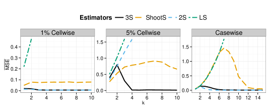
Figure 1: $\overline{MSE}$ for various cellwise and casewise contamination values, $k$, for models with continuous covariates. The sample size is $n=300$.

Table 1 shows the $\overline{MSE}$ for clean data and the maximum $\overline{MSE}$ for all the cellwise and casewise contamination settings for $n=150,300$. Figure 1 shows the curves of $\overline{MSE}$ for various cellwise and casewise contamination values for $n=300$. The results for $n=150$ are similar and the corresponding figure is shown as supplementary material.

In the cellwise contamination setting, 3S-regression is highly robust against moderate and large cellwise outliers ($k\geq 3$), but less robust against inliers ($k\leq 2$). Notice that inliers also affect the performance of the shooting S-estimator but to a lesser extent. Since the filter does not flag inliers, 3S-regression and 2S-regression perform similarly in the presence of inliers (see the central panel of Figure 1). The shooting S-estimator is highly robust against large outliers, but less so against moderate cellwise outliers. As expected, 2S-regression breaks down in the case of $\epsilon=0.05$, when the propagation of large cellwise outliers is expected to affect more than 50% of the cases.

In the casewise contamination setting, 2S-regression has the best performance, as expected. 3S-regression also performs fairly well in this setting. The shooting S-estimator performs less satisfactorily in this case.

We have also considered other simulation settings and observed similar results (not shown here). In particular, we considered $p=5$ with $n=50,100$ and $p=25$ with $n=250,500$ under the same set of scenarios (clean data, cellwise contamination, and casewise contamination). Moreover, we studied the performance of 3S-regression for larger casewise contamination levels up to 20%. 3S-regression maintains its competitive performance, outperforming Shooting S and not falling too far behind 2S-regression, which is expected to win in these situations.

5.1.2 Performance of confidence intervals

We then assess the performance of confidence intervals for the regression coefficients based on the asymptotic covariance matrix as described in Section 4. Intervals that have a coverage close to the nominal value, while being relatively short, are desirable.

The $100(1-\tau)\%$ confidence interval (CI) of 3S-regression has the form:

$$CI(\hat{\beta}_{j})=\left[\hat{\beta}_{j}-\Phi^{-1}(1-\tau/2)\sqrt{\widehat{ASV}(\hat{\beta}_{j})/n},\,\,\hat{\beta}_{j}+\Phi^{-1}(1-\tau/2)\sqrt{\widehat{ASV}(\hat{\beta}_{j})/n}\right],$$

for $j=0,1,\dots,p$, where $\hat{\beta}_{0}=\hat{\alpha}$. We consider $\tau=0.05$ here. We evaluate the performance of CI using the Monte Carlo mean coverage rate (CR):

$$\overline{CR}=\frac{1}{N}\sum_{m=1}^{N}\frac{1}{p}\sum_{j=1}^{p}I(\beta_{j}^{(m)}\in CI(\hat{\beta}_{j}^{(m)})),$$

and the Monte Carlo mean CI lengths:

$$\overline{CIL}=\frac{1}{N}\sum_{m=1}^{N}\frac{1}{p}\sum_{j=1}^{p}2\Phi^{-1}(1-\tau/2)\sqrt{\widehat{ASV}(\hat{\beta}_{j})/n}.$$

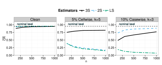
Figure 2: $\overline{CR}$ for clean data and for cellwise and casewise contaminated data of various sample size, $n$.

Figure 2 shows the $\overline{CR}$ in the case of clean data, 5% cellwise contamination ($k=5$), and 10% casewise contamination ($k=3$) simulation, with different sample sizes $n=150,300,500,1000$. The nominal value of 95% is indicated by the horizontal line in the figure.

For clean data, the coverage rates of all the intervals reach the nominal level when the sample size grows, as expected. For data with casewise outliers, 2S-regression yields the best coverage rate, which is closest to the nominal level. However, 3S-regression has an acceptable performance, comparable with that of 2S-regression. For data with cellwise outliers, 3S-regression yields intervals with a coverage rate relatively closer to the nominal value than LS and 2S-regression.

Table 2: Average lengths of confidence intervals for clean data and for cellwise and casewise contamination.

	Clean		1% Cell., $k=5$		5% Cell., $k=5$		10% Case., $k=3$
Size ($n$)	3S	2S	3S	2S	3S	2S	3S	2S
150	0.341	0.352	0.355	0.402	0.450	1.519	0.329	0.355
300	0.242	0.247	0.244	0.275	0.294	1.148	0.239	0.253
500	0.187	0.189	0.190	0.212	0.222	0.912	0.189	0.197
1000	0.133	0.133	0.134	0.150	0.155	0.662	0.137	0.140

Furthermore, the length of the intervals obtained from 3S regression is comparable to that LS for clean data and that of 2S-regression for clean data and data with casewise outliers. For data with cellwise outliers, 3S-regression yields intervals with lengths relatively closer to the case of clean data. Table 2 shows the average lengths of the confidence intervals obtained from 3S- and 2S-regression in the case of clean data, 1% cellwise contamination ($k=5$), 5% cellwise contamination ($k=5$), and 10% casewise contamination ($k=3$) simulation, with different sample sizes $n=150,300,500,1000$. The results of LS are not included here.

In general, 3S-regression yields slightly shorter intervals than 2S-regression in all scenarios because the asymptotic variance is calculated on the data with the filtered cells imputed instead of the complete data. On the other hand, 2S-regression tends to yield longer intervals in the cellwise contamination model, even when the propagation of outliers is below the 0.5 breakdown point under THCM, for example, when $\varepsilon=0.01$. This maybe because 2S-regression loses a significant amount of clean data for estimation when it down-weights cases with outlying components.

5.2 Models with continuous and dummy covariates

We now conduct a simulation study to assess the performance of our procedure when the model includes continuous and dummy covariates. We consider the regression model in (8) with $p_{x}=12$, $p_{d}=3$, and $n=150,300$. The random covariates $(\boldsymbol{X}_{i},\boldsymbol{D}_{i})$, $i=1,\dots,n$, are first generated from multivariate normal distribution $N_{p}(\boldsymbol{0},\boldsymbol{\Sigma})$, where $\boldsymbol{\Sigma}$ is the randomly generated correlation matrix with a fixed condition number of 100. Then, we dichotomize $D_{ij}$ at $\Phi^{-1}(\pi_{j})$ where $\pi_{j}=\frac{1}{4},\frac{1}{3},\frac{1}{2}$ for $j=1,2,3$, respectively. Finally, the rest of data are generated in the same way as described in Section 5.1.

In the simulation study, we consider the following scenarios:

• Clean data: No further changes are done to the data;

• Cellwise contamination: Randomly replace a $\epsilon$ fraction of the cells in $\mathbb{X}$ by outliers $X_{ij}^{cont}=E(X_{ij})+k\times SD(X_{ij})$ and $\epsilon$ proportion of the responses by outliers $Y_{ij}^{cont}=E(Y_{ij})+k\times SD(\varepsilon_{i})$, where $k=1,2,\dots,10$;

• Casewise contamination: Let $\boldsymbol{\Sigma}_{x}$ be the sub-matrix of $\boldsymbol{\Sigma}$ with rows and columns corresponding to the continuous covariates. Randomly replace a $\epsilon$ fraction of the cases in $\mathbb{X}$ by leverage outliers ${\boldsymbol{X}_{i}^{cont}}=c\boldsymbol{v}$, where $\boldsymbol{v}$ is the eigenvector corresponding to the smallest eigenvalue of $\boldsymbol{\Sigma}_{x}$ with length such that $(\boldsymbol{v}-\boldsymbol{\mu}_{x})^{t}\boldsymbol{\Sigma}^{-1}(\boldsymbol{v}-\boldsymbol{\mu}_{x})=1$. In this case, the number of continuous variables is 13 (instead of 16) and the corresponding least favorable casewise contamination size is found to be $c=7$ (instead of 8) using the same procedure as in Section 5.1. Finally, we replace the corresponding response value by $Y_{i}^{cont}={\boldsymbol{X}_{i}^{cont}}^{t}\boldsymbol{\beta}_{x}+\boldsymbol{D}_{i}^{t}\boldsymbol{\beta}_{d}+\varepsilon_{i}^{cont}$ with $\varepsilon_{i}^{cont}\sim N(k,\sigma^{2})$, where $k=1,2,\dots,10$.

Again, we consider $\epsilon=0.01,0.05$ for cellwise contamination, and $\epsilon=0.10$ for casewise contamination. The number of replicates for each setting is $N=1000$.

Table 3: Maximum $\overline{MSE}$ in all the considered scenarios for models with continuous and dummy covariates.

	Clean		1% Cellwise		5% Cellwise		Casewise
$n=$	150	300	150	300	150	300	150	300
3S	0.010	0.004	0.018	0.008	0.636	0.507	0.090	0.071
ShootS	0.012	0.005	0.026	0.015	0.746	0.468	0.450	0.387
2S	0.008	0.003	0.014	0.007	1.894	1.341	0.060	0.054
LS	0.007	0.003	2.785	2.532	5.162	4.981	1.332	1.322

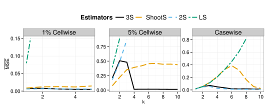
Figure 3: $\overline{MSE}$ for various cellwise and casewise contamination values, $k$, for models with continuous and dummy covariates. The sample size is $n=300$.

Table 3 shows the $\overline{MSE}$ for clean data and the maximum $\overline{MSE}$ for all the cellwise and casewise contamination settings for $n=150,300$. Figure 3 shows the curves of $\overline{MSE}$ for various cellwise and casewise contamination values for $n=300$. The results for $n=150$ are similar and the corresponding figure is shown as supplementary material. Overall, 3S-regression remains competitive in the case of continuous and dummy covariates.

We also consider the case of non-normal covariates. The covariates are generated from several asymmetric distributions, and the data are contaminated in a similar fashion. The performance of 3S-regression in the case of non-normal covariates is similar to the performance in the case of normal covariates. Results are available as supplementary material.

6 Analysis of the Boston housing data

We illustrate the effect of cellwise outlier propagation on classical robust estimators using the Boston Housing data. The data, available at the UCI repository (Bache and Lichman, 2013), was collected from 506 census tracts in the Boston Standard Statistical Metropolitan Area in the 1970s on 14 different features. We consider the nine quantitative variables that were extensively studied (e.g., see in Öllerer et al., 2015). The variables are listed and described in Table 2 in the supplementary material. There is no missing data. The original objective of the study in Harrison and Rubinfeld (1978) was to analyze the association between the median housing values (medv) in Boston and the residents’ willingness to pay for clean air.

We fit the following model using 3S-regression, the shooting S-estimator, 2S-regression and the LS estimator:

$$log(medv)=\alpha +\beta_{1}\,log(crim)+\beta_{2}\,nox^{2}+\beta_{3}\,rm^{2}+\beta_{x,4}\,age$$

$$+\beta_{5}\,log(dis)+\beta_{6}\,tax+\beta_{7}\,ptratio+\beta_{8}\,black+\beta_{9}\,log(lstat)+\varepsilon.$$

The regression coefficient estimates and their P-values are given in Table 4. In particular, we observe that the regression coefficients for the covariates $age$ and $black$ are very different under 3S and 2S-regression. Moreover, $age$ is significant under 2S-regression but highly non-significant under 3S-regression. 2S-regression is somewhat inefficient because it throws away a substantial amount of clean data due to the propagation of cellwise outliers. It fully down-weights 16.4% of the cases in the dataset (cases that receive a zero weight by the multivariate S-estimator). Slightly more than half of these cases (8.7%) are affected by the propagation of cellwise outliers mainly in the covariates $nox^{2}$ and $black$ (1.3% of the cells in the dataset are flagged by the consistent filter). After filtering, these cases have relatively small partial Mahalanobis distances, indicating they are close to the bulk of the data for the remaining variables.

Table 4: Estimates and p-values of the regression coefficients for the original Boston Housing data.

Variable	3S		ShootS		2S		LS
	Coeff.	P-Val.	Coeff.	P-Val.	Coeff.	P-Val.	Coeff.	P-Val.
log(lstat)	-0.243	$<$0.001	-0.266	-	-0.153	$<$0.001	-0.395	$<$0.001
rm2	0.015	$<$0.001	0.013	-	0.018	$<$0.001	0.007	$<$0.001
tax	-0.051	$<$0.001	-0.021	-	-0.046	$<$0.001	-0.028	0.006
log(dis)	-0.125	$<$0.001	-0.157	-	-0.126	$<$0.001	-0.139	$<$0.001
ptratio	-0.026	$<$0.001	-0.027	-	-0.025	$<$0.001	-0.029	$<$0.001
nox2	-0.578	0.013	-0.463	-	-0.445	0.023	-0.451	$<$0.001
age	-0.023	0.645	-0.040	-	-0.152	0.001	0.050	0.391
black	-0.726	0.398	0.787	-	-0.007	0.993	0.500	$<$0.001
log(crim)	-0.006	0.513	0.004	-	0.005	0.527	-0.002	0.813

We further compare the four estimators by computing their squared norm distances, $n\times\sum_{j=1}^{p}(\widehat{\beta}_{j,A}-\widehat{\beta}_{j,B})^{2}\times MAD(\{X_{1j},\dots,X_{nj}\})^{2}$ (see Öllerer et al., 2015), where $MAD$ is the median absolute deviation. Table 5 shows the squared norm distances for the considered estimators. Overall, the three robust estimators are very different from LS. As expected, 3S-regression and shooting S are closer to each other than they are to 2S-regression. Additional analysis provided as supplementary material indicates that the observed differences between the three robust estimators are indeed mostly caused by the propagation of cellwise outliers in the Boston housing data.

Table 5: Pairwise squared norm distances between the estimates for the original Boston housing data.

	3S	ShootS	2S	LS
3S	-	1.389	3.145	6.725
ShootS		-	4.312	4.661
2S			-	16.614
LS				-

7 Concluding remarks

High breakdown point affine equivariant robust estimators are neither efficient nor robust in the independent cellwise contamination model (ICM). By efficiency here we mean the ability to use the clean part of the data. In fact, classical robust estimators are inefficient under ICM because they may down-weight an entire row with a single component being contaminated. Therefore, they may lose some useful information contained in the data. Furthermore, the classical high breakdown point affine equivariant robust estimators may break down under ICM. A small fraction of cellwise outliers could propagate, affecting a large proportion of cases. For instance, the probability $\overline{\epsilon}$ that at least one component of a case is contaminated is $\overline{\epsilon}=1-(1-\epsilon)^{p}$, where $\epsilon$ is the proportion of independent cellwise outliers. This implies that even if $\epsilon$ is small, $\overline{\epsilon}$ could be large for large $p$, and could exceed the 0.5 breakdown point under THCM. For example, if $\epsilon=0.1$ and $p=10$, then $\overline{\epsilon}=0.65$; and if $\epsilon=0.05$ and $p=20$, then $\overline{\epsilon}=0.64$.

To overcome these deficiencies of the classical robust estimators, we introduce a three-step regression estimator that can deal with cellwise and casewise outliers. The first step of our estimator is aimed at reducing the impact of outliers propagation posed by ICM. The second step is aimed at achieving robustness under THCM. As a result, the robust regression estimate from the third step is shown to be efficient (in terms of data usage) and robust under ICM and THCM. We also prove that our estimator is consistent and asymptotically normal at the central regression model distribution. Finally, we extend our estimator to models with continuous and dummy covariates and provide an algorithm to compute the regression coefficients.

The proposed procedures are implemented in the R package robreg3S, which is freely available on CRAN (the Comprehensive R Archive Network, R Core Team, 2015).

References

- Agostinelli et al. (2015) Agostinelli, C., Leung, A., Yohai, V. J., Zamar, R. H., 2015. Robust estimation of multivariate location and scatter in the presence of cellwise and casewise contamination. TEST 24 (3), 441–461.
- Alqallaf et al. (2009) Alqallaf, F., Van Aelst, S., Yohai, V. J., Zamar, R. H., 2009. Propagation of outliers in multivariate data. Ann Statist 37 (1), 311–331.
- Bache and Lichman (2013) Bache, K., Lichman, M., 2013. UCI machine learning repository. http://archive.ics.uci.edu/ml.
- Croux et al. (2003) Croux, C., van Aelst, S., Dehon, C., 2003. Bounded influence regression using high breakdown scatter matrices. Ann Inst Statist Math 55, 265–285.
- Danilov (2010) Danilov, M., 2010. Robust estimation of multivariate scatter under non-affine equivarint scenarios. Ph.D. thesis, University of British Columbia.
- Danilov et al. (2012) Danilov, M., Yohai, V. J., Zamar, R. H., 2012. Robust estimation of multivariate location and scatter in the presence of missing data. J Amer Statist Assoc 107, 1178–1186.
- Davies (1987) Davies, P., 1987. Asymptotic behaviour of S-estimators of multivariate location parameters and dispersion matrices. Ann Statist 15, 1269–1292.
- Farcomeni (2014a) Farcomeni, A., 2014a. Robust constrained clustering in presence of entry-wise outliers. Technometrics 56, 102–111.
- Farcomeni (2014b) Farcomeni, A., 2014b. Snipping for robust K-means clustering under component-wise contamination. Stat Comp 24, 909–917.
- Farcomeni (2015) Farcomeni, A., 2015. Comments on: Robust estimation of multivariate location and scatter in the presence of cellwise and casewise contamination. TEST.
- Fu (1998) Fu, W., 1998. Penalized regressions: The bridge versus the lasso. J Comput Graph Statist 7 (3), 397–416.
- Gervini and Yohai (2002) Gervini, D., Yohai, V. J., 2002. A class of robust and fully efficient regression estimators. Ann Statist 30 (2), 583–616.
- Harrison and Rubinfeld (1978) Harrison, D., Rubinfeld, D. L., 1978. Hedonic prices and the demand for clean air. J Environ Econ Manage 5, 81–102.
- Huber and Ronchetti (2009) Huber, P. J., Ronchetti, E. M., 2009. Robust Statistics (2nd edition). John Wiley & Sons, New Jersey.
- Leung et al. (2015) Leung, A., Danilov, M., Yohai, V., Zamar, R., 2015. GSE: Robust Estimation in the Presence of Cellwise and Casewise Contamination and Missing Data. R package version 3.2.3.
- Lopuhaä (1989) Lopuhaä, H. P., 1989. On the relation between S-estimators and M-estimators of multivariate location and covariance. Ann Statist 17, 1662–1683.
- Maronna and Morgenthaler (1986) Maronna, R. A., Morgenthaler, S., 1986. Robust regression through robust covariance matrices. Comm Statist Theory Methods 15, 1347–1365.
- Maronna and Yohai (2000) Maronna, R. A., Yohai, V. J., 2000. Robust regression with both continuous and categorical predictors. J Statist Plann Inference 89, 197–214.
-
Öllerer et al. (2015)
Öllerer, V., Alfons, A., Croux, C., 2015. The shooting S-estimator for
robust regression. Comput Statist.
URL http://dx.doi.org/10.1007/s00180-015-0593-7 -
R Core Team (2015)
R Core Team, 2015. R: A Language and Environment for Statistical Computing. R
Foundation for Statistical Computing, Vienna, Austria.
URL http://www.R-project.org/ - Rousseeuw (1984) Rousseeuw, P., 1984. Least median of squares regression. J Amer Statist Assoc 79, 871–880.
- Rousseeuw and Yohai (1984) Rousseeuw, P. J., Yohai, V. J., 1984. Robust regression by means of S-estimators. In: Franke, J., Härdle, W., Martin, D. (Eds.), Robust and Nonlinear Time Series. Vol. 26 of Lecture Notes in Statistics. Springer, New York, US, pp. 256–272.
- Ruppert and Simpson (1990) Ruppert, D., Simpson, D., 1990. Unmasking multivariate outliers and leverage points: Comment. J Amer Statist Assoc 85, 644–646.
-
Todorov and Filzmoser (2009)
Todorov, V., Filzmoser, P., 2009. An object-oriented framework for robust
multivariate analysis. Journal of Statistical Software 32 (3), 1–47.
URL http://www.jstatsoft.org/v32/i03/ -
Venables and Ripley (2002)
Venables, W. N., Ripley, B. D., 2002. Modern Applied Statistics with S, 4th
Edition. Springer, New York, iSBN 0-387-95457-0.
URL http://www.stats.ox.ac.uk/pub/MASS4 - Yohai (1985) Yohai, V. J., 1985. High breakdown point and high efficiency robust estimates for regression. Tech. Rep. 66, Department of Statistics, University of Washington, available at http://www.stat.washington.edu/research/reports/1985/tr066.pdf.