Fuzzy Jets

Abstract

Collimated streams of particles produced in high energy physics experiments are organized using clustering algorithms to form jets. To construct jets, the experimental collaborations based at the Large Hadron Collider (LHC) primarily use agglomerative hierarchical clustering schemes known as sequential recombination. We propose a new class of algorithms for clustering jets that use infrared and collinear safe mixture models. These new algorithms, known as fuzzy jets, are clustered using maximum likelihood techniques and can dynamically determine various properties of jets like their size. We show that the fuzzy jet size adds additional information to conventional jet tagging variables. Furthermore, we study the impact of pileup and show that with some slight modifications to the algorithm, fuzzy jets can be stable up to high pileup interaction multiplicities.

1 Introduction

As the result of a proton-proton collision at a hadron collider, hundreds of particles are created and detected Aad:2010ac ; Khachatryan:2010nk . While some particles can be identified by their type, such as electrons Khachatryan:2015hwa ; Aad:2014nim and muons Chatrchyan:2012xi ; Aad:2014rra , most of the detected particles are light hadrons produced in collimated sprays called jets. Jets are the consequence of high energy quarks or gluons fragmenting into colorless hadrons. Experimentally, jets are defined by clustering schemes which group together measured calorimeter energy deposits or reconstructed charged particle tracks. A jet algorithm is a clustering scheme that connects the measured objects with theoretical quantities that can be calculated and simulated. At a hadron collider, the natural coordinates for describing particles are $p_{T}$, $y$, and $\phi$, where $p_{T}$ is the magnitude of the momentum transverse to the proton beam, $y$ is the rapidity, and $\phi$ is the azimuthal angle. Particles or calorimeter energy deposits are clustered using jet algorithms based on distance metrics on their coordinates in $(p_{T},\vec{\rho})=(p_{T},y,\phi)$. In order for a jet algorithm to be useful to experimentalists and theorists, the collection of jets should be IRC safe in the following sense:

1. Infrared safe (IR): if a particle $i$ is added with $|p_{T}|\rightarrow 0$, the jets are unaffected.

2. Collinear safe (C): if a particle $i$ with momentum $p_{i}$ is replaced with two particles $j$ and $k$ with momenta $p_{j}+p_{k}=p_{i}$ such that $|\vec{\rho}_{i}-\vec{\rho}_{j}|=0$, then the jets are unaffected.

The jet algorithms most widely used at hadron colliders fall into a class of schemes known as sequential recombination Ellis:1993tq . These IRC safe schemes require metrics $d$ on momenta $d_{ij}=d(p_{i},p_{j}):(p_{i},p_{j})\rightarrow\mathbb{R}^{+},d_{iB}=d(p_{i}):p_{i}\rightarrow\mathbb{R}^{+}$ and proceed as follows:

1. Assign each particle as a proto-jet.

2. Repeat until there are no proto-jets left: Let $(k,\ell)=\text{argmin}_{i,j}d(p_{i},p_{j})$ and without loss of generality, $d_{kB}<d_{\ell B}$. If $d_{kB}<d_{k\ell}$, declare proto-jet $k$ a jet and remove it from the list. Otherwise, combine proto-jets $k$ and $\ell$ into a new proto-jet with momentum $p_{\text{new}}=p_{\ell}+p_{k}$.

One common prescription is called the Cambridge-Aachen (C/A) algorithm Dokshitzer:1997in ; Wobisch:1998wt , which uses $d_{ij}=|\vec{\rho}_{i}-\vec{\rho}_{j}|^{2}/R^{2}$ and $d_{iB}=1$. The fixed quantity $R$ is roughly the size of the jet in $(y,\phi)$. By far, the most ubiquitous jet algorithm used at the Large Hadron Collider (LHC) is the anti-$k_{t}$ algorithm Cacciari:2008gp with $d_{ij}=\min(p_{T,i}^{-2},p_{T,j}^{-2})|\vec{\rho}_{i}-\vec{\rho}_{j}|^{2}/R^{2}$ and $d_{iB}=p_{T,i}^{-2}$.

The purpose of this paper is to introduce a new paradigm for jet clustering, called fuzzy jets, based on probabilistic mixture modeling. Section 2 introduces the statistical concept of a mixture model and describes the necessary modification to make the procedure IRC safe. Section 3 gives one efficient method for clustering fuzzy jets based on the Expectation-Maximization (EM) algorithm. Section 4.4 contains several examples comparing fuzzy jets with sequential recombination and Sec. 5 describes how one might mitigate the impact of overlapping proton-proton collisions (pileup). We conclude in Sec. 6 with some summary remarks and outlook for the future.

2 Mixture Model Jets

Mixture models opac-b1097397 are a statistical tool for clustering which postulate a particular class of probability densities for the data to be clustered. Generically, for grouping $m$ $n$-dimensional data points into $k$ clusters, the mixture model density is

$$p(x_{1},...,x_{m}|\theta)=\prod_{i=1}^{m}\left(\sum_{j=1}^{k}\pi_{j}f(x_{i}|\theta_{j})\right),$$ (1)

where $\pi_{j}$ is the unknown weight of cluster $j$ such that $\sum_{j}\pi_{j}=1$ and $f(x_{i}|\theta_{j})$ is a probability density on $n$-dimensions with unknown parameters $\theta_{j}$ to be learned from the data. A common choice for $f$ is the normal density $\Phi$ with $\theta_{j}=(\mu_{j},\Sigma_{j})$ for $\mu_{j}$ the $n$-dimensional mean and $\Sigma_{j}$ the $n\times n$ covariance matrix. In the mixture model paradigm, the $\theta_{j}$ are the cluster properties; in the Gaussian case, $\mu_{j}$ is the location of cluster $j$ and $\Sigma_{j}$ describes its shape in the $n$-dimensional space. When clustering with a finite mixture, the number of clusters $k$ must be specified ahead of time, which is dual to the usual use of sequential recombination in which $k$ is learned and the size of jets is specified ahead of time. The standard objective in (frequentist) mixture modeling is to select the parameters $\theta_{j}$ which maximize the likelihood (Eq. 1) of the observed dataset. Figure 1 illustrates what the learned event density might look like for $k=3$ and Gaussian $f=\Phi$ in $n=2$ dimensions.

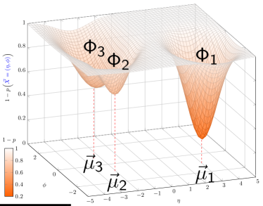
Figure 1: An example of the learned per-particle probability density specified in Eq. (1) with $k=3$ and Gaussian $f=\Phi$ in $n=2$ dimensions. One cluster is associated with each component density $\Phi_{i}=\Phi(\cdot\mid\mu_{i},\Sigma_{i})$, where the dot $\cdot$ is a placeholder for the function argument.

An equivalent way of approaching mixture modeling is to view Eq. (1) as the density used to generate the data. We view the data as having been drawn randomly from the density specified in Eq. (1), with the following setup:

1. Throw $n$ independent and identical $k$-sided dice with probability $\pi_{j}$ to land on side $j=1,...,k$ and label the outcomes $\lambda_{1},...,\lambda_{n}$.

2. Independent of the others, data point $i\in\{1,...,n\}$ is drawn randomly from $f(\cdot\mid\theta_{\lambda_{i}})$.

Once $\theta$ and $\pi$ are learned by minimizing Eq. (1), we can compute $q_{ij}=\Pr(\lambda_{i}=j\mid x_{i})$, the posterior probability that $x_{i}$ was generated by $f(\cdot\mid\theta_{j})$ or, intuitively, the posterior probability that $x_{i}$ belongs to cluster $j$. The $q_{ij}$ are the soft assignments of particles $i$ to jet $j$ and will play an important role in Sec. 3 when we show how to maximize the likelihood in Eq. (1). Jets produced with mixture modeling are called fuzzy jets because of the soft memberships - every particle can belong to every jet with some probability. This can be seen explicitly in Fig. 1 where the densities of all three clusters are everywhere nonzero, so $q_{ij}>0$ for all $j$. The idea of probabilistic membership was recently studied in the context of the Q-jets algorithm Ellis:2012sn in which the same event is interpreted many times by injecting randomness into the clustering procedure. Unlike Q-jets, fuzzy jets allocates the soft membership functions deterministically throughout the clustering procedure. However, like Q-jets, there is an ambiguity in how to assign kinematic properties to the clustered jets. Fuzzy jets are defined by their shape (and location), not their constituents. This is in contrast to anti-$k_{t}$ jets, which are defined by their constituents without an explicit shape determined from the clustering procedure. One simple assignment scheme is to define the momentum of a fuzzy jet $j$ as

$$p_{\text{jet $j$}}=\sum_{i=1}^{m}p_{i}\left\{\begin{matrix}1&j=\text{argmax}_{k}q_{ik}\cr 0&\text{else}\end{matrix}\right\}.$$ (2)

In other words, this procedure assigns every particle to its most probable associated jet. This scheme will be known as the hard maximum likelihood (HML) scheme, but is not the only possible assignment algorithm. The dual problem in sequential recombination is the jet area, which must be defined areas , whereas the jet kinematics are the ‘natural’ coordinates.

We now specialize the likelihood in Eq. (1) to the case of clustering particles into jets at a collider like the LHC. Consider a mixture model in two dimensions with $x_{i}=\rho_{i}$. The resulting mixture model (MM) jets are inherently not IR safe: particle $p_{T}$ does not appear in the likelihood and therefore arbitrarily low energy particles can influence the clustering procedure. Therefore, we add a modification to the log likelihood:

$$\log\mathcal{L}(\{p_{T,i},\rho_{i}\}|\theta)=\sum_{i=1}^{m}p_{T,i}^{\alpha}\log\left(\sum_{j=1}^{k}\pi_{j}f(\rho_{i}|\theta_{j})\right),$$ (3)

where $\alpha$ is a weighting factor. Equation (3) is the log of Eq. (1) with the term $p_{T,i}^{\alpha}$ inserted in the outer sum. For $\alpha>0$, the resulting modified mixture model (mMM) jets are IR safe, and when $\alpha=1$, the jets are C safe. Therefore, for $\alpha=1$, the jets are IRC safe. Different choices of component densities $f$ in Eq. (3) give rise to different IRC safe MM jet algorithms. We have studied several possibilities for $f$, but for the remainder of this paper will specialize to (wrappedfootnote 4) Gaussian $f=\Phi$. The resulting fuzzy jets are called modified Gaussian Mixture Model jets (mGMM) and are parameterized by the locations $\mu_{j}$, the covariance matrices $\Sigma_{i}$, and the cluster weights $\pi_{j}$. We initialize $\pi_{j}=1/k$ and $\Sigma_{j}=I$.

Since practical procedures for maximizing the modified likelihood in Eq. (3) may converge to stationary points that are not globally optimal, the output of a fuzzy jet algorithm will depend on an initial setting of the cluster parameters $\theta$ and $\pi$. One simple procedure, used exclusively for the rest of the paper, is to seed fuzzy jets based on the output of a sequential recombination jet algorithm. This guarantees an IRC safe initial condition and therefore the entire procedure is IRC safe. We now discuss practically how one can find the maximum of the fuzzy jets likelihood.

3 Clustering Fuzzy Jets: the EM Algorithm

One iterative procedure for maximizing the mixture model likelihood in Eq. (1) is the Expectation-Maximization (EM) algorithm em1 ; em2 ; em3 . After initializing the cluster locations and prior density $\pi$, the following two steps are repeated:

Expectation

Given the current values of $\theta_{j}$, compute the fuzzy membership probabilities $q_{ij}=\pi_{j}\Phi(\vec{\rho}_{i}|\mu_{j},\Sigma_{j})/\sum_{j^{\prime}}\pi_{j^{\prime}}\Phi(\vec{\rho}_{i}|\mu_{j^{\prime}},\Sigma_{j^{\prime}})$.

Maximization

Given $q_{ij}$, maximize the expected modified complete log likelihood over the parameters $\pi,\mu,\Sigma$.

The expected modified complete log likelihood has the form

$$\sum_{i=1}^{N}\sum_{j=1}^{k}p_{Ti}^{\alpha}(q_{ij}\log\Phi(\vec{\rho}_{i};\vec{\mu}_{j},\Sigma_{j})+q_{ij}\log\pi_{j}).$$ (4)

Note that the expected modified complete log likelihood is not the same as the expected modified log likelihood, shown in Eq. (3). They differ in that the complete log likelihood has the second sum outside the logarithm while Eq. (3) has the sum inside the logarithm. The power of the EM algorithm is that maximizing the complete log likelihood results in fixed point iteration to monotonically improve the original log likelihood. This desirable property of the EM algortihm is still true when $\alpha>0$; for a proof, see Appendix B. Many choices for $f$ have closed form maxima for the M step; in the Gaussian $f=\Phi$ case outlined above, the updates are given by

$$\mu_{j}^{*}=\sum_{i=1}^{n}\tilde{q}_{ij}x_{i}\hskip 19.91692pt\Sigma_{j}^{*}=\sum_{i=1}^{n}\tilde{q}_{ij}(x_{i}-\mu_{j})(x_{i}-\mu_{j})^{\mathsf{T}}\hskip 19.91692pt\pi_{j}^{*}=\frac{1}{\sum_{i=1}^{n}p_{Ti}^{\alpha}}\sum_{i=1}^{n}p_{Ti}^{\alpha}\tilde{q}_{ij},$$ (5)

where $\tilde{q}_{ij}=q_{ij}p_{Ti}^{\alpha}/\sum_{l=1}^{n}p_{lj}p_{Tl}^{\alpha}$. The well-known $k$-means clustering algorithm macqueen1967 can be recovered as the limit of expectation-maximization in a Gaussian mixture model with $\Sigma=\sigma^{2}I,\sigma^{2}\rightarrow 0$. Figure 2 illustrates GMM clustering using the EM algorithm with $k=2$ clusters. The EM algorithm readily accommodates constraints on the model parameters. One constraint we will consider throughout the rest of the paper is $\Sigma_{j}=\sigma_{j}^{2}I$ for all $j$, which requires the curves of constant likelihood in $(y,\phi)$ to be circular. We will see in the next section that the learned value of $\sigma_{j}$ is useful for distinguishing jets originating from different physics processes.

\begin{overpic}[width=86.72267pt]{figs/Init.pdf} \put(18.0,90.0){\scriptsize Initialization} \end{overpic}

\begin{overpic}[width=86.72267pt]{figs/Estep} \put(25.0,90.0){\scriptsize$1^{\text{st}}$ E step} \end{overpic}

\begin{overpic}[width=86.72267pt]{figs/Mstep} \put(25.0,90.0){\scriptsize$1^{\text{st}}$ M step} \end{overpic}

\begin{overpic}[width=86.72267pt]{figs/Estep2} \put(25.0,90.0){\scriptsize$2^{\text{nd}}$ E step} \end{overpic}

\begin{overpic}[width=86.72267pt]{figs/Mstep2} \put(25.0,90.0){\scriptsize$2^{\text{nd}}$ M step} \par\put(-305.0,0.0){ \par \leavevmode\hbox to171.52pt{\vbox to86.16pt{\text{[drawing]}}} \par} \par\put(-105.0,0.0){ \par \leavevmode\hbox to171.52pt{\vbox to86.16pt{\text{[drawing]}}} \par} \par\end{overpic}

\begin{overpic}[width=86.72267pt]{figs/Estep3} \put(25.0,90.0){\scriptsize$3^{\text{rd}}$ E step} \end{overpic}

\begin{overpic}[width=86.72267pt]{figs/Mstep3} \put(25.0,90.0){\scriptsize$3^{\text{rd}}$ M step} \end{overpic}

\begin{overpic}[width=86.72267pt]{figs/Estep4} \put(25.0,90.0){\scriptsize$4^{\text{th}}$ E step} \end{overpic}

\begin{overpic}[width=86.72267pt]{figs/Mstep4} \put(25.0,90.0){\scriptsize$4^{\text{th}}$ M step} \end{overpic}

\begin{overpic}[width=86.72267pt]{figs/Mstep5} \put(21.0,103.0){\scriptsize$5^{\text{st}}$ M step:} \put(22.0,90.0){\scriptsize\color[rgb]{1,0,0} Converged} \par\put(-405.0,0.0){ \par \leavevmode\hbox to171.52pt{\vbox to86.16pt{\text{[drawing]}}} \par} \par\put(-205.0,0.0){ \par \leavevmode\hbox to171.52pt{\vbox to86.16pt{\text{[drawing]}}} \par} \par\end{overpic}

Figure 2: An illustration of of the EM algorithm for $k=2$. The circles represent data points, the triangles represent the estimated cluster locations $\mu_{j}$, and the ellipsoids are equidensity contours describing the shapes $\Sigma_{j}$ of the learned cluster distributions. In the E-step, bluer colors correspond to higher value of $p_{i,\text{\color[rgb]{0,0,1} blue jet}}$.

4 Comparisons with Sequential Recombination and Jet Tagging

This section describes some numerical comparisons between sequential recombination and fuzzy jets. Section 4.1 summarizes the simulation details with some first event displays showing both fuzzy and sequential recombination jets. These two approaches to jet clustering are studied over an ensemble of events in Sec. 4.2. A third subsection, Sec. 4.3, illustrates that fuzzy jets captures new information about the hadronic final state, and in the fourth section, Sec 4.4, it is demonstrated that this new information can be used to classify the jet type.

4.1 Details of the Simulation

In order to study fuzzy jets in a realistic scenario, we run Monte Carlo (MC) simulations. Three physics processes are generated using Pythia 8.170 Pythia8 ; Pythia at $\sqrt{s}=8$ TeV. Hadronic $W$ boson and top quarks are used for studying hard 2- and 3-prong type jets, respectively. To simulate high $p_{T}$ hadronic $W$ decays, $W^{\prime}$ bosons are generated to decay exclusively into a $W$ and $Z$ boson which subsequently decay into quarks and leptons, respectively. The $p_{T}$ scale of the hadronically decaying $W$ is set by the mass of the $W^{\prime}$ which is tuned to 800 GeV for this study so that the $p_{T}^{W}\lesssim 400$ GeV. In this $p_{T}^{W}$ range, the $W$ decay products are expected to merge within a cone of $R~{}1.0$ where $\Delta R^{2}=\Delta\phi^{2}+\Delta\eta^{2}\sim 4m_{W}^{2}/p_{T,W}^{2}$. A sample enriched in 3-prong type jets is generated with $Z^{\prime}\rightarrow t\bar{t}$, where the $Z^{\prime}$ mass sets the energy scale of the hadronically decaying top quarks. In this analysis, we use $m_{Z^{\prime}}=1.0$ TeV, which sets $p_{T}^{t}\gtrsim 500$ GeV. To study the impact on signal versus background, QCD dijets are generated with a range of $\hat{p}_{T}$ that is approximately in the same range as the relevant signal process. In all distributions, the QCD $p_{T}$ spectrum is weighted to exactly match that of the signal to control for differences between signal and background due only to the $p_{T}$ spectrum differences. Pileup is simulated by overlaying additional independently generated minimum-bias interactions with each signal event. For the rest of this section, the number of pileup interactions $n_{\text{PU}}=0$. See Sec. 5 for studies of $n_{\text{PU}}>0$.

For a comparison to fuzzy jets, anti-$k_{t}$ jets are clustered using FastJet fastjet 3.0.3. The signal processes are chosen such that jets with radius parameter $R=1$ are most appropriate in capturing the decay products of the heavy particles. The anti-$k_{t}$ jets are trimmed trimming by re-clustering the constituents into $R=0.3$ $k_{t}$ subjets and dropping those which have $p_{T}^{\text{subjet}}<0.05\times p_{T}^{\text{jet}}$. Anti-$k_{t}$ jets are also used to seed the fuzzy jet clustering; the $p_{T}$ threshold for this initialization is 5 GeV, and the impact of this choice is studied in Appendix C.

To model the discretization and finite acceptance of a real detector, a calorimeter of towers with size $0.1\times 0.1$ in $(y,\phi)$ extends out to $y=5.0$. The total energy of the simulated particles incident upon a particular cell are added as scalars and the four-vector $p_{j}$ of any particular tower $j$ is given by

$$p_{j}=\sum_{i\text{ incident on $j$}}E_{i}(\cos\phi_{j}/\cosh y_{j},\sin\phi_{j}/\cosh y_{j},\sinh y_{j}/\cosh y_{j},1).$$ (6)

To simulate a particle flow reconstruction, the sum in Eq. (6) contains only neutral particles for $|y|<2.5$ and both charged and neutral particles for $2.5<|y|<5$. Charged particles within $|y|<2.5$ are individually added to the list of inputs for clustering, unless they originate from a pileup collision. Anti-$k_{t}$ jet momenta are corrected for pileup on average using area subtraction areas . The median pileup density, $\rho$, is estimated by clustering hard scatter particles, neutral pileup particles, and charged pileup particles in the range $|y|<2.5$ using $k_{t}$ $R=0.4$ jets in FastJet with ghosted areas.

\begin{overpic}[width=216.81pt]{figs/draft_figs/PaperED_mGMMc_1_0_notracker.pdf} \put(12.0,98.0){\Large\emph{Pythia 8}} \put(12.0,91.0){$\sqrt{s}=8\text{ TeV}$} \put(62.0,91.0){\large$\text{Z'}\rightarrow\text{t}\bar{\text{t}}$} \par\put(24.0,-4.0){\small Pseudorapidity ($\eta$)} \put(-4.0,18.0){\rotatebox{90.0}{\small Rotated Azimuthal Angle ($\phi$)}} \put(95.0,25.0){\rotatebox{90.0}{\small Particle $p_{T}\text{ [GeV]}$}} \par\put(5.0,8.0){\small$0$} \put(4.0,28.3){\small$\frac{\pi}{2}$} \put(5.0,48.3){\small$\pi$} \put(4.0,68.0){\small$\frac{3\pi}{2}$} \put(4.0,88.0){\small$2\pi$} \par\put(4.0,4.0){\small$-3$} \put(17.0,4.0){\small$-2$} \put(29.6,4.0){\small$-1$} \put(46.2,4.0){\small$0$} \put(58.8,4.0){\small$1$} \put(71.3,4.0){\small$2$} \put(83.8,4.0){\small$3$} \par\end{overpic}

\begin{overpic}[width=216.81pt]{figs/draft_figs/PaperED_mGMMc_1_0_akt.pdf} \put(12.0,98.0){\Large\emph{Pythia 8}} \put(12.0,91.0){$\sqrt{s}=8\text{ TeV}$} \put(62.0,91.0){\large$\text{Z'}\rightarrow\text{t}\bar{\text{t}}$} \par\put(24.0,-4.0){\small Pseudorapidity ($\eta$)} \put(-4.0,18.0){\rotatebox{90.0}{\small Rotated Azimuthal Angle ($\phi$)}} \put(95.0,25.0){\rotatebox{90.0}{\small Particle $p_{T}\text{ [GeV]}$}} \par\put(5.0,8.0){\small$0$} \put(4.0,28.3){\small$\frac{\pi}{2}$} \put(5.0,48.3){\small$\pi$} \put(4.0,68.0){\small$\frac{3\pi}{2}$} \put(4.0,88.0){\small$2\pi$} \par\put(4.0,4.0){\small$-3$} \put(17.0,4.0){\small$-2$} \put(29.6,4.0){\small$-1$} \put(46.2,4.0){\small$0$} \put(58.8,4.0){\small$1$} \put(71.3,4.0){\small$2$} \put(83.8,4.0){\small$3$} \end{overpic}

Figure 3: A representative event display for a $Z^{\prime}\rightarrow t\bar{t}$ event. In the top left plot, gray circles show the location and size of mGMM fuzzy jets after clustering, with the size of the circle indicating 1-$\sigma$ contours in the detector; the black circle indicates the highest $p_{T}$ jet with HML particle assignment. The small filled colored circles are the particles, with the color and size indicating their energy. In each case, the events have been rotated in $\phi$ to place the truth top quark at $\phi=3\pi/2$, which is indicated by a red star. Anti-$k_{t}$ jet locations are shown with gray crosses in the left hand plot, the long tail of which points towards the mGMM jet for which it was a seed. In the top right plot, anti-$k_{t}$ R = 1.0 jets passing a $5$ GeV $p_{T}$ cut are shown as discs under the particles indicating their active area, with centers the same as the crosses in the left hand side. Shades of gray in the anti-$k_{t}$ discs have no scale and are meant to aid the eye, but go from low $p_{T}$ (lighter) to high $p_{T}$ (darker).

A representative event display for a $Z^{\prime}\rightarrow t\bar{t}$ event is shown in Figure 3. The top right plot in Figure 3 shows the anti-$k_{t}$ jets with $p_{T}>5$ GeV as filled in (partial) circles. The filled area is determined by the jet area and there are deviations from circles only one a low $p_{T}$ jet is close to a higher $p_{T}$ jet. The two top quarks are depicted as red stars, each of which sits at the center of two high $p_{T}$ jets. The top left plot in Figure 3 shows mGMM fuzzy jets. The fuzzy jets are depicted by their 1-$\sigma$ contours. In contrast to the anti-$k_{t}$ jets, fuzzy jets vary widely in radial size. Gray crosses in the top left plot indicate the locations of the anti-$k_{t}$ jets shown in the top right plot. The long tail of the crosses point toward the fuzzy jet for which they were the seed. The two jets closest to the top quarks did not move a long distance from the seed location, though the size did change significantly from $R=1$. The lowest $p_{T}$ fuzzy jet moved a long distance from the seed to the final location.

Another new feature of fuzzy jets compared to anti-$k_{t}$ jets is that they can overlap with each other. This is seen by the four jets with overlapping 1-$\sigma$ contours in the top left plot of Figure 3. Overlapping mGMM jets are an expression of structure inadequately captured with a single Gaussian shape. The ability to learn features at different scales in the same event without relying on a size parameter like the anti-$k_{t}$ radius parameter can give mGMM fuzzy jets additional descriptive power over anti-$k_{t}$ and other traditional jet algorithms. This particular event will be used again for reference in Section 5 during a discussion on the performance of the technique in the presence of pileup interactions.

4.2 Kinematic Properties of Fuzzy Jets

Jets clustered according to the mGMM algorithm capture similar hard jet locations and jet energy (under HML) as those clustered by anti-$k_{t}$ $R=1$. In Figure 4, the $p_{T}$ distribution for the highest $p_{T}$ jets for three different physics processes are plotted as given by anti-$k_{t}$ $R=1.0$ and mGMM jets. The anti-$k_{t}$ $p_{T}$ distributions are re-weighted so that all three processes have identical distributions in the left plot. On the right, the distributions are in good correspondence with those in the left plot, though there is a slight shift of the peak. Additionally, the $(y,\phi)$ locations of the highest $p_{T}$ mGMM jets are in excellent correspondence with the locations of the anti-$k_{t}$ jets as was already discussed in reference to Figure 3.

Figure 4: The jet $p_{T}$ for the leading anti-$k_{t}$ jet (left) and leading fuzzy jet under the HML particle assignment scheme (right). All the processes are re-weighted so that the anti-$k_{t}$ $p_{T}$ spectra are the same.

The mGMM algorithm differs from the anti-$k_{t}$ algorithm in how the size and structure of clustered jets. This was already shown qualitatively in Figure 3: fuzzy jets come in a variety of sizes, and can overlap in complex ways. The matter is further complicated by the choice of particle assignment scheme for defining kinematic properties in the mGMM family of algorithms. The catchment area’s volume and shape of a fuzzy jet depends in general on the full set of learned jet locations and model parameters, $\Sigma$. In contrast, for anti-$k_{t}$ jets, the catchment area is bounded from above by $R$ and is only smaller when another high $p_{T}$ jet is nearby. The nonlocality of the mGMM clustering model can be observed quantitatively by examining jet mass, given in Eq. (7), which is sensitive to the distribution of energy within a jet. The jet mass distributions for both mGMM (HML assignment) and anti-$k_{t}$ jets are shown in Figure 5, with the same $p_{T}$ weighting as in Figure 4. Even though fuzzy jets learn the same core (i.e. $p_{T}$) for jets as anti-$k_{t}$, they do not learn the same mass. The white dashed lines in Figure 5 mark the locations of the $W$ boson and top quark masses at about 80 GeV and 175 GeV, respectively Agashe:2014kda . For both anti-$k_{t}$ and fuzzy jets, there are clear peaks at the $W$ mass for the boosted $W\rightarrow qq^{\prime}$ from $W^{\prime}$ simulated events and at the top quark mass for $Z^{\prime}\rightarrow t\bar{t}$ simulated events. However, there are clear differences in the shape of these distributions. The $W$ mass peak for $W^{\prime}$ events is more peaked for fuzzy jets, though there is also a low-mass contribution to the distribution. For $Z^{\prime}$ events, the top quark mass peak is less populated for fuzzy jets, which instead has shifted events to the $W$ mass peak. This often happens when the tree-prong structure is learned by two (overlapping) fuzzy jets. The QCD multi-jet jet mass distribution is also qualitatively different between fuzzy jets and anti-$k_{t}$ jets, with the former shifted to lower values of the mass.

$$m_{\text{jet}}^{2}=\left(\sum_{i\in\text{jet}}E_{i}\right)^{2}-\left(\sum_{i\in\text{jet}}\vec{p}_{i}\right)^{2}$$ (7)

Figure 5: The jet mass for the leading anti-$k_{t}$ (left) and leading fuzzy jet under the HML particle assignment scheme (right), in an anti-$k_{t}$ leading jet $p_{T}$ window of 350 to 450 GeV. All the processes are re-weighted so that the anti-$k_{t}$ $p_{T}$ distributions are the same. The dashed white lines mark $m_{W}=80.4\text{ GeV}$ and $m_{t}=173.3\text{ GeV}$.

4.3 New Information from Fuzzy Jets

The properties $\Sigma$ of a fuzzy jet can be useful in distinguishing jets resulting from different physics processes. In the simplest realization of mGMM jets already described above, $\Sigma=\sigma^{2}I$, where $\sigma$ is a measure of the size of the core of a jet. Although $\sigma$ is a simple variable to construct from the wealth of data available after clustering with the mGMM algorithm, it captures at least some of the schematic differences in the likelihood for $Z^{\prime}\rightarrow t\bar{t}$ and $W^{\prime}\rightarrow WZ$ relative to a QCD multijet background (shown below).

The left plot of Figure 6 also shows the average $\sigma$ over all fuzzy jets in an event. The generic fuzzy jet is rather independent of the physics process and tends to be quite large. This is because fuzzy jets capturing hard radiation tend to be small, but most of the fuzzy jets needed to capture the sparse radiation pattern from the underlying event need to be large. In contrast, the $\sigma$ for the leading mGMM jets are shown the right plot of Figure 6 for each of the three physics processes. As expected, the decay relative size of the highest $p_{T}$ jets depends on the physics process. For the decay of a boosted heavy particle with mass $m$ and $p_{T}$, the radial size of the decay products scales as $2m/p_{T}$ and thus since the $p_{T}$ distribution in Figure 6 is fixed, one would expect that the top quark jets have a larger $\sigma$ than the $W$ boson jets, which are in turn larger than the quark and gluon jets. This is reflected in the three peaks in the left plot of Figure 6. The separation between the three physics processes it not 100% correlated with the naive scaling $m/p_{T}$ of the corresponding leading anti-$k_{t}$ jets. Figure 7 shows that there is a strong positive correlation between $\sigma$ and the corresponding anti-$k_{t}$ mass over $p_{T}$ as expected. There are two peaks in the correlation for the $Z^{\prime}\rightarrow t\bar{t}$ events because the anti-$k_{t}$ mass spectrum has peaks at both the top mass, and the $W$ boson mass. While the correlations between the fuzzy jet $\sigma$ and the anti-$k_{t}$ $m/p_{T}$ are non-negligible, they are far from unity and thus there may be additional information contained in the fuzzy jet $\sigma$ that is useful for tagging the flavour of a jet.

Figure 6: The learned value of $\sigma$ for the highest $p_{T}$ jet under the HML scheme (left) and for all jets (right) for various physics processes.

\begin{overpic}[width=186.45341pt]{figs/draft_figs/zprime_sigma_rho_correlation.pdf} \put(18.0,5.0){\small Leading Anti-$k_{t}$ Jet $m/p_{T}$} \put(4.0,30.0){\rotatebox{90.0}{\small Leading Learned $\sigma$}} \put(99.0,30.0){\rotatebox{90.0}{\small Arbitrary Units}} \put(62.0,93.0){\large$\text{Z'}\rightarrow\text{t}\bar{\text{t}}$} \par\put(20.0,82.0){\Large\emph{Pythia 8}} \put(20.0,75.0){$\sqrt{s}=8\text{ TeV}$} \put(18.0,70.0){\tiny$350\leq p_{T}^{\text{Jet}}\leq 450\text{ GeV}$} \par\put(45.0,20.0){\small$\rho_{\sigma,\text{m}/p_{T}}=0.679$} \end{overpic}

\begin{overpic}[width=186.45341pt]{figs/draft_figs/qcd_sigma_rho_correlation.pdf} \put(18.0,5.0){\small Leading Anti-$k_{t}$ Jet $m/p_{T}$} \put(4.0,30.0){\rotatebox{90.0}{\small Leading Learned $\sigma$}} \put(99.0,30.0){\rotatebox{90.0}{\small Arbitrary Units}} \put(69.0,93.0){\large$\text{QCD}$} \par\put(20.0,82.0){\Large\emph{Pythia 8}} \put(20.0,75.0){$\sqrt{s}=8\text{ TeV}$} \put(18.0,70.0){\tiny$350\leq p_{T}^{\text{Jet}}\leq 450\text{ GeV}$} \par\put(45.0,20.0){\small$\rho_{\sigma,\text{m}/p_{T}}=0.688$} \end{overpic}

Figure 7: The left and right plots show the correlation between $\sigma$ and the leading jet anti-$k_{t}$ mass divided by $p_{T}$ in an anti-$k_{t}$ $p_{T}$ window of $350$ to $450$ GeV for $Z^{\prime}\rightarrow t\bar{t}$ and QCD events, respectively. Indicated in the lower right of each figure is the linear correlation between the variables.

4.4 Fuzzy Jets for Tagging

In this section, $\sigma$ is compared with another class of jet substructure variables known to be useful for tagging: the $N$-subjettiness ratios nsub . $N$-subjettiness moments are defined over a set of $N$ axes, and calculated as:

$$\tau_{N}=\frac{1}{d_{0}}\sum_{k}p_{T,k}\min\{\Delta R_{1,k},\Delta R_{2,k},\ldots\Delta R_{N,k}\},$$ (8)

where $d_{0}$ is the normalization

$$d_{0}=\sum_{k}p_{T,k}R_{0},$$ (9)

and $R_{0}$ is the radius of the jet. In practice, the useful variables for determining how much more $i$-pronged a jet is compared to $j$-pronged are the $N$-subjettiness ratios:

$$\tau_{ij}=\frac{\tau_{i}}{\tau_{j}}.$$ (10)

The variable $\tau_{21}$ is often used for the separation of $W$ from QCD jets wbosonCMS ; wbosonATLAS and is a measure of the compatibility of a jet with a 2-prong hypothesis compared to a 1-prong hypothesis. Low value of $\tau_{21}$ indicates that the jet likely has a 2-prong structure. Similarly, $\tau_{32}$ is useful for top tagging in that it measures whether a 3-prong structure is a better description of a jet relative to a 2-prong structure.

The rest of his section contains comparisons of the performance of $\sigma$ relative to $\tau_{21}$ for separating $W$ from QCD jets, as well as $\sigma$ relative to $\tau_{32}$ for tagging $Z^{\prime}\rightarrow t\bar{t}$ amongst a QCD jet background. In Figure 8, a $k$-nearest neighbors classifier was trained with 2-fold cross validation in TMVA Hocker:2007ht . The left plot in Figure 8 demonstrates an increase in performance for discriminating $Z^{\prime}\rightarrow t\bar{t}$ from QCD relative to using $\tau_{32}$ alone. The fuzzy jet $\sigma$ is roughly equally useful to the $N$-subjettiness ratio at a sigma efficiency of $0.85$, and using both variables greatly improves background rejection. Similar results can be seen in the right plot of Figure 8, where $\sigma$ boosts background rejection relative to $\tau_{21}$ alone. In each case, the training and classification was performed in a mass window around the particles of interest, the top quark mass in the $Z^{\prime}\rightarrow t\bar{t}$ sample and the $W$ boson mass to discriminate $W\rightarrow qq^{\prime}$ from QCD.

Figure 8: The tagging performance of $\sigma$ relative to $\tau_{32}$ ($\tau_{21}$) for distinguishing top quarks ($W$ bosons) from a QCD background is shown on the left (right). The random tagger keeps a fixed fraction of all events, regardless of their origin and is a lower bound on the performance of any tagger.

The comparisons of the fuzzy jet $\sigma$ and $N$-subjettiness are intended to be an illustrative example. As discussed in the opening of this section, $\sigma$ is just one variable that can be constructed by using mGMM clustered jets. Expanded studies of the various learned parameters could come up with additional variables, or the full learned parameter set could be thrown into an off the shelf classifier or machine learning model.

5 Underlying Event and Pileup

As with any new jet algorithm or jet variable, understanding the effect of pileup vertices from additional proton-proton collisions is essential to make meaningful statements about how the method will be applicable to real data analyses at the LHC. Studying pileup in the context of mGMM jets is complicated by the effective catchment area of the jets. For hierarchical-agglomerative algorithms like anti-$k_{t}$, the catchment area scales with the radius parameter. However fuzzy jets can have infinite catchment area because the likelihood for particle membership is nonzero for any finite distance and arrangement of Gaussian jets and particles. Furthermore, the catchment area can change depending on the other jets in an event. Although this effect also occurs in the hierarchical-agglomerative case, the effect is much more pronounced in the mGMM clustering algorithm, with some jets having finite catchment areas while others cluster infinite area.

The challenge of pileup for fuzzy jets is illustrated in Figure 9, where the same event is shown with $n_{\text{PU}}=0$, and with $n_{\text{PU}}=40$. The event displays show the central region of the detector, where most of the decay products of the hard scatter lie. Qualitatively, it can be seen that the introduction of additional interaction vertices broadens all of the mGMM jets. This broadening clearly impacts the power of $\sigma$ for differentiating QCD background from signal processes.

\begin{overpic}[width=186.45341pt]{figs/draft_figs/PaperED_mGMMc_1_0.pdf} \put(12.0,98.0){\Large\emph{Pythia 8}} \put(12.0,91.0){$\sqrt{s}=8\text{ TeV}$} \put(62.0,91.0){\large$\text{Z'}\rightarrow\text{t}\bar{\text{t}}$} \put(62.0,98.0){\large$n_{\text{PU}}=0$} \par\put(24.0,-4.0){\small Pseudorapidity ($\eta$)} \put(-4.0,10.0){\rotatebox{90.0}{\small Rotated Azimuthal Angle ($\phi$)}} \put(95.0,27.0){\rotatebox{90.0}{\small Tower $p_{T}\text{ [GeV]}$}} \par\put(5.0,8.0){\small$0$} \put(4.0,28.3){\small$\frac{\pi}{2}$} \put(5.0,48.3){\small$\pi$} \put(4.0,68.0){\small$\frac{3\pi}{2}$} \put(4.0,88.0){\small$2\pi$} \par\put(4.0,4.0){\small$-3$} \put(17.0,4.0){\small$-2$} \put(29.6,4.0){\small$-1$} \put(46.2,4.0){\small$0$} \put(58.8,4.0){\small$1$} \put(71.3,4.0){\small$2$} \put(83.8,4.0){\small$3$} \end{overpic}

\begin{overpic}[width=186.45341pt]{figs/draft_figs/PaperED_mGMMc_1_40.pdf} \put(12.0,98.0){\Large\emph{Pythia 8}} \put(12.0,91.0){$\sqrt{s}=8\text{ TeV}$} \put(62.0,91.0){\large$\text{Z'}\rightarrow\text{t}\bar{\text{t}}$} \put(59.0,98.0){\large$n_{\text{PU}}=40$} \par\put(24.0,-4.0){\small Pseudorapidity ($\eta$)} \put(-4.0,10.0){\rotatebox{90.0}{\small Rotated Azimuthal Angle ($\phi$)}} \put(95.0,27.0){\rotatebox{90.0}{\small Tower $p_{T}\text{ [GeV]}$}} \par\put(5.0,8.0){\small$0$} \put(4.0,28.3){\small$\frac{\pi}{2}$} \put(5.0,48.3){\small$\pi$} \put(4.0,68.0){\small$\frac{3\pi}{2}$} \put(4.0,88.0){\small$2\pi$} \par\put(4.0,4.0){\small$-3$} \put(17.0,4.0){\small$-2$} \put(29.6,4.0){\small$-1$} \put(46.2,4.0){\small$0$} \put(58.8,4.0){\small$1$} \put(71.3,4.0){\small$2$} \put(83.8,4.0){\small$3$} \end{overpic}

Figure 9: mGMM jets defined according to Section 2 with an isotropic kernel are broadened as a result of the introduction of additional $pp$ pileup vertices. The same hard scatter is clustered twice, on the left with $n_{\text{PU}}=0$ and on the right with $n_{\text{PU}}=40$. Vertical dashed lines at $\eta=\pm 2.5$ show the extent of a simulated tracker with the same $\eta$ extent as that used at ATLAS and CMS. Charged pileup falling within the extent of the simulated tracker is discarded before clustering and the aggregation of particles into towers.

The next sections explore two methods for mitigating the impact of pileup in relation to fuzzy jets, illustrated with the variable $\sigma$.

5.1 Changing $\alpha$ for Pileup Suppression

In Section 2, it was discussed that choosing $\alpha=1$ in the likelihood (Eq. (3)) guarantees IRC safety. With $\alpha=1$, the mGMM algorithm treats hard structure and soft structure linearly in the particle or tower $p_{T}$. However, one can exploit the fact that $\sigma$ is disproportionately a measure of the shape and extent of the leading jet hard structure to make the variable more resilient to the effects of pileup. In particular, choosing $\alpha>1$ stabilizes $\sigma$ at high $n_{\text{PU}}$ because so long as the average input particle $p_{T}$ due to pileup is significantly smaller than the $p_{T}$ of the particles constituting the leading jet hard structure, the change in likelihood will be suppressed roughly according to $\left(p_{T,\text{hs}}/p_{T,\text{PU}}\right)^{\alpha}$. An example of this effect is illustrated in Figure 10, which shows the same event as in Figure 9. The price for adjusting $\alpha$ is the loss of collinear safety. Varying $\alpha$ is not explored further, as Section 5.2 demonstrates a method for dealing with pileup effectively that does not rely on moving $\alpha$ away from the IRC safe value of one.

\begin{overpic}[width=186.45341pt]{figs/draft_figs/PaperED_mGMMc_1_0_alpha2.pdf} \put(12.0,98.0){\Large\emph{Pythia 8}} \put(12.0,91.0){$\sqrt{s}=8\text{ TeV}$} \put(62.0,91.0){\large$\text{Z'}\rightarrow\text{t}\bar{\text{t}}$} \put(62.0,98.0){\large$n_{\text{PU}}=0$} \put(68.8,105.0){\large$\alpha=2$} \par\put(24.0,-4.0){\small Pseudorapidity ($\eta$)} \put(-4.0,10.0){\rotatebox{90.0}{\small Rotated Azimuthal Angle ($\phi$)}} \put(95.0,27.0){\rotatebox{90.0}{\small Tower $p_{T}\text{ [GeV]}$}} \par\put(5.0,8.0){\small$0$} \put(4.0,28.3){\small$\frac{\pi}{2}$} \put(5.0,48.3){\small$\pi$} \put(4.0,68.0){\small$\frac{3\pi}{2}$} \put(4.0,88.0){\small$2\pi$} \par\put(4.0,4.0){\small$-3$} \put(17.0,4.0){\small$-2$} \put(29.6,4.0){\small$-1$} \put(46.2,4.0){\small$0$} \put(58.8,4.0){\small$1$} \put(71.3,4.0){\small$2$} \put(83.8,4.0){\small$3$} \end{overpic}

\begin{overpic}[width=186.45341pt]{figs/draft_figs/PaperED_mGMMc_1_40_alpha2.pdf} \put(12.0,98.0){\Large\emph{Pythia 8}} \put(12.0,91.0){$\sqrt{s}=8\text{ TeV}$} \put(62.0,91.0){\large$\text{Z'}\rightarrow\text{t}\bar{\text{t}}$} \put(59.0,98.0){\large$n_{\text{PU}}=40$} \put(68.8,105.0){\large$\alpha=2$} \par\put(24.0,-4.0){\small Pseudorapidity ($\eta$)} \put(-4.0,10.0){\rotatebox{90.0}{\small Rotated Azimuthal Angle ($\phi$)}} \put(95.0,27.0){\rotatebox{90.0}{\small Tower $p_{T}\text{ [GeV]}$}} \par\put(5.0,8.0){\small$0$} \put(4.0,28.3){\small$\frac{\pi}{2}$} \put(5.0,48.3){\small$\pi$} \put(4.0,68.0){\small$\frac{3\pi}{2}$} \put(4.0,88.0){\small$2\pi$} \par\put(4.0,4.0){\small$-3$} \put(17.0,4.0){\small$-2$} \put(29.6,4.0){\small$-1$} \put(46.2,4.0){\small$0$} \put(58.8,4.0){\small$1$} \put(71.3,4.0){\small$2$} \put(83.8,4.0){\small$3$} \end{overpic}

Figure 10: Clustering in the mGMM model with $\alpha=2$. There is little broadening between the $n_{\text{PU}}=0$ (left) and $n_{\text{PU}}=40$ (right) cases, but jets at the locations of the tops in the event are substantially narrower than in the case where $\alpha=1$, even with $n_{\text{PU}}=0$ (compare to Figure 9). Under the ML particle assignment, the $\alpha=2$ algorithm identifies the other top as the highest $p_{T}$ jet in the event, demonstrating the difficulty in dealing with fuzzy jet kinematics.

5.2 Tower Subtraction and the Event Jet: Effective Pileup Correction

Recent developments in pileup mitigation have led to several algorithms for correcting jet inputs before jet clustering beings. Such techniques include Pileup Per Particle Identification (PUPPI), Constituent Subtraction, and SoftKiller puppi ; constsub ; softkill . One simple input-correction scheme is to subtract from each calorimeter tower the estimated pileup $p_{T}$ density per unit area multiplied by the size of the tower in the detector. As a first step, $\rho$ is calculated in the same way as described in Sec. 4.1. Tower momenta are then corrected according to Eq. (11), where $p_{T,\text{s}}$ is the corrected momentum, $p_{T,\text{o}}$ is the original momentum, and $A$ is the area of the tower. In this study, all towers have area $0.1\times 0.1$ in $y$-$\phi$ space.

$$p_{T,\text{s}}=\text{max}\left(p_{T,\text{o}}-\rho A,0\right).$$ (11)

While subtracting the average $p_{T}$ background from towers before clustering is a relatively safe way of reducing the effect of pileup, at least when the $p_{T}$ scales of the tower to tower fluctuations are small compared to the hard scatter $p_{T}$ scale, it would still be helpful to systematically address the question of catchment areas. The mGMM clustering algorithm provides a natural framework in which to think about pileup, however, because the algorithm deals fundamentally with likelihoods, and the pileup likelihood is to leading order uniform over the detector (this is the motivation for the area-subtraction technique). This is the motivation for modifying the mGMM likelihood using a technique we call the event jet.

In addition to learning $k$ mGMM jets throughout clustering, the event jet includes another background contribution to the likelihood which attempts to capture the intuition of a uniform contribution of particle likelihood due to pileup. Constraints are further imposed on the likelihood on the event level jet so that it has constant likelihood during the clustering process, making the necessary modifications to the algorithm procedures simpler.

Practically, the effect of the event jet can be parameterized through the introduction of an algorithmic parameter $\gamma$. Particle membership probabilities change according to Eq. (12) with corresponding changes to the analytical M step for the Gaussian kernel type. The choice of $\gamma$ is important, and it should reflect the fact that not all events are created equal in the sense that not all events have the same contributions due to pileup. Although there is no strict way of dealing with this issue, it is reasonable to replace $\gamma$ by a meaningful combination of parameters which is sensitive to our estimates of the amount of pileup in a particular event. We have chosen to take $\gamma=\rho A\gamma_{w}$ where $\rho$ is our estimate of the $p_{T}$ density due to pileup, $A$ is the calorimeter area, and $\gamma_{w}$ is a parameter of the algorithm controlling the strength of the event jet. Initial studies with the event jet indicate that introducing a $\rho$ dependent $\gamma$ is much more effective than a $\rho$ independent one.

$$q_{ij}\rightarrow\frac{q_{ij}}{\gamma+\sum_{k}p_{ik}}$$ (12)

\begin{overpic}[width=186.45341pt]{figs/draft_figs/PaperED_mGMMc_1_0_corr.pdf} \put(12.0,98.0){\Large\emph{Pythia 8}} \put(12.0,91.0){$\sqrt{s}=8\text{ TeV}$} \put(62.0,91.0){\large$\text{Z'}\rightarrow\text{t}\bar{\text{t}}$} \put(62.0,98.0){\large$n_{\text{PU}}=0$} \put(55.0,105.0){\large Corrected} \par\put(24.0,-4.0){\small Pseudorapidity ($\eta$)} \put(-4.0,10.0){\rotatebox{90.0}{\small Rotated Azimuthal Angle ($\phi$)}} \put(95.0,27.0){\rotatebox{90.0}{\small Tower $p_{T}\text{ [GeV]}$}} \par\put(5.0,8.0){\small$0$} \put(4.0,28.3){\small$\frac{\pi}{2}$} \put(5.0,48.3){\small$\pi$} \put(4.0,68.0){\small$\frac{3\pi}{2}$} \put(4.0,88.0){\small$2\pi$} \par\put(4.0,4.0){\small$-3$} \put(17.0,4.0){\small$-2$} \put(29.6,4.0){\small$-1$} \put(46.2,4.0){\small$0$} \put(58.8,4.0){\small$1$} \put(71.3,4.0){\small$2$} \put(83.8,4.0){\small$3$} \end{overpic}

\begin{overpic}[width=186.45341pt]{figs/draft_figs/PaperED_mGMMc_1_40_corr.pdf} \put(12.0,98.0){\Large\emph{Pythia 8}} \put(12.0,91.0){$\sqrt{s}=8\text{ TeV}$} \put(62.0,91.0){\large$\text{Z'}\rightarrow\text{t}\bar{\text{t}}$} \put(59.0,98.0){\large$n_{\text{PU}}=40$} \put(55.0,105.0){\large Corrected} \par\put(24.0,-4.0){\small Pseudorapidity ($\eta$)} \put(-4.0,10.0){\rotatebox{90.0}{\small Rotated Azimuthal Angle ($\phi$)}} \put(95.0,27.0){\rotatebox{90.0}{\small Tower $p_{T}\text{ [GeV]}$}} \par\put(5.0,8.0){\small$0$} \put(4.0,28.3){\small$\frac{\pi}{2}$} \put(5.0,48.3){\small$\pi$} \put(4.0,68.0){\small$\frac{3\pi}{2}$} \put(4.0,88.0){\small$2\pi$} \par\put(4.0,4.0){\small$-3$} \put(17.0,4.0){\small$-2$} \put(29.6,4.0){\small$-1$} \put(46.2,4.0){\small$0$} \put(58.8,4.0){\small$1$} \put(71.3,4.0){\small$2$} \put(83.8,4.0){\small$3$} \end{overpic}

Figure 11: Jet correction using tower subtraction and the event jet with parameter $\gamma_{w}=0.01$. The two leading $p_{T}$ jets are almost identical in size in the left and right insets, which show the $n_{\text{PU}}=0$ and $n_{\text{PU}}=40$ cases respectively. Although many of the other jets change (including the migration of jets to higher $\left|\eta\right|$ as a result of the simulated tracker), those that give the $\sigma$ and sub-leading $\sigma$ variables are insensitive to the effect of pileup.

Studies of the pileup conditions similar to LHC Run I, with $\sim 20$ pileup interactions, indicate that with a 5 GeV $p_{T}$ cut, $\gamma_{w}=0.01$ provides reasonable stability of the learned $\sigma$. This is demonstrated qualitatively in Figure 11, in which the tower and event jet corrections are applied to the same event shown in Figure 3 at both $n_{\text{PU}}=0$ and $n_{\text{PU}}=40$. Unlike any of the methods discussed previously, this method for correction maintains IRC safety, demonstrates very little jet broadening at $n_{\text{PU}}=40$, and is not drastically different in its qualitative features by comparison to the standard mGMM algorithm. Note that the assignment of towers to jets under the HML scheme is impacted with the event jet because many towers belong to the event jet with higher probability than any of the other fuzzy jets. To preserve tower-to-jet assignments under pileup, a smaller value of $\gamma_{w}$ should be chosen. The event jet is useful instead because it changes the dynamics of clustering, making jets less sensitive to soft radiation far away from the jet axis during the EM update steps, and therefore increasing the stability of the hard core that is eventually clustered.

A quantitative study of the pileup mitigation suggested qualitatively by Figure 11 requires an ensemble of events. Figure 12 shows how the mean and standard deviation of learned $\sigma$ evolve with $n_{\text{PU}}$. The uncorrected $\sigma$ is shown in red downward pointing triangles while the tower subtraction and event jet corrections are shown in blue upward pointing triangles. For both $Z^{\prime}\rightarrow t\bar{t}$ and QCD, the pileup dependence is dramatically reduced with the tower subtraction and the event jet. The uncorrected mean $\sigma$ increases as a function of $n_{\text{PU}}$ as all of the fuzzy jets become the same size. The standard deviation of the uncorrected $\sigma$ actually decreases beyond $n_{\text{PU}}\sim 5$ as all of the fuzzy jets become the same size. For modest levels of pileup, tower subtraction and event and the event jet maintain the mean and standard deviation of the $\sigma$ distribution.

Figure 12: For both QCD and $Z^{\prime}\rightarrow t\bar{t}$ samples, using the pileup correction (blue triangles) via the event jet and tower subtraction stabilizes the mean relative to the uncorrected samples (red inverted triangles), and prevents widening of the $\sigma$ distribution in pileup conditions somewhat worse than during Run 1 at the LHC.

6 Conclusions

The modified mixture model algorithms provide a new way of looking at whole event structure. In contrast to the usual uses of hierarchical-agglomerative algorithms like anti-$k_{t}$, the number of seeds is fixed ahead of time and their properties are learned during the clustering process. The learned parameters provide a new set of handles for distinguishing jets of different types. Even simple variables constructed out of the learned parameters of a mixture of isotropic Gaussian jets, like $\sigma$, offer complementary information to the $n$-subjettiness variables $\tau_{21}$ and $\tau_{32}$ for tagging $W$ boson and top quark jets. Even though the variable $\sigma$ is sensitive to changes in pileup conditions, small modifications to the fuzzy jets algorithm – correcting jet inputs and adding a pileup likelihood – can mitigate the impact of pileup.

Fuzzy jets are new paradigm for jet clustering in high energy physics. These IRC safe likelihood-based clustering schemes set the stage for many possibilities for future studies related to jet tagging, probabilistic clustering, and pileup suppression.

7 Acknowledgments

We would like to thank Jesse Thaler for useful discussions and helpful feedback on the manuscript. In addition, we thank Gavin Salam for useful comments on the algorithm description. This work is supported by the US Department of Energy (DOE) Early Career Research Program and grant DE-AC02-76SF00515. BN is supported by the NSF Graduate Research Fellowship under Grant No. DGE-4747 and by the Stanford Graduate Fellowship.

Appendix A Wrapped Gaussian

In the EM algorithm described in Sec. 3, there are explicit (and implicit) dependencies on the topology. For instance, if a Gaussian density is used to model $\phi$, then, in the E step, a particle with $\phi_{i}$ near $2\pi$ will be deemed far from a cluster with location $\phi_{j}$ near $0$. To avoid this undesirable behavior and enforce the equivalence of the angles $0$ and $2\pi$, we associate $\phi$ with a wrapped Gaussian density and $y$ with a standard Gaussian density:

$$\Phi(y,\phi|\mu_{\phi},\mu_{y},\sigma^{2})=\Phi_{y}(y|\mu_{y},\sigma^{2})\frac{1}{\sqrt{2\pi\sigma^{2}}}\sum_{I=-\infty}^{\infty}\exp\left[\frac{-(\phi-\mu_{\phi}(I))^{2}}{2\sigma^{2}}\right],$$ (13)

where $\Phi_{y}$ is a normal distribution and $\mu_{\phi}(I)=\mu_{\phi}+2\pi I$. In order to approximate the sum in Eq. (13), we take only the leading contribution by choosing $\mu_{\phi}(I^{*})$ for $I^{*}=\text{argmin}_{I^{\prime}}|\phi-\mu_{\phi}+2\pi I^{\prime}|$. As other contributions are exponentially suppressed, this is a good approximation and recovers continuity near $0$ and $2\pi$. Figure 13 illustrates the improved clustering behavior that results when $\phi$ is modeled using the wrapped Gaussian approximation in place of the standard Gaussian density.

\begin{overpic}[width=186.45341pt]{figs/draft_figs/PaperED_pifix_ed_0_unfixed.pdf} \put(11.0,91.0){\small Naive Gaussian Density} \put(72.2,50.8){\tiny{\color[rgb]{0.8,0.8,0.8}Internal}} \put(70.0,46.2){\tiny{\color[rgb]{0.8,0.8,0.8}boundary}} \put(24.0,-4.0){\small Pseudorapidity ($\eta$)} \put(-4.0,10.0){\rotatebox{90.0}{\small Rotated Azimuthal Angle ($\phi$)}} \put(95.0,37.0){\rotatebox{90.0}{\small$p_{T}\text{ [GeV]}$}} \par\put(5.0,8.0){\small$\pi$} \put(4.0,28.3){\small$\frac{3\pi}{2}$} \put(4.0,48.3){\small$2\pi$} \put(4.0,68.0){\small$\frac{5\pi}{2}$} \put(4.0,88.0){\small$3\pi$} \par\put(4.0,4.0){\small$-3$} \put(17.0,4.0){\small$-2$} \put(29.6,4.0){\small$-1$} \put(46.2,4.0){\small$0$} \put(58.8,4.0){\small$1$} \put(71.3,4.0){\small$2$} \put(83.8,4.0){\small$3$} \end{overpic}

\begin{overpic}[width=186.45341pt]{figs/draft_figs/PaperED_pifix_ed_0_fixed.pdf} \put(11.0,91.0){\small Wrapped Approximation} \put(72.2,50.8){\tiny{\color[rgb]{0.8,0.8,0.8}Internal}} \put(70.0,46.2){\tiny{\color[rgb]{0.8,0.8,0.8}boundary}} \put(24.0,-4.0){\small Pseudorapidity ($\eta$)} \put(-4.0,10.0){\rotatebox{90.0}{\small Rotated Azimuthal Angle ($\phi$)}} \put(95.0,37.0){\rotatebox{90.0}{\small$p_{T}\text{ [GeV]}$}} \par\put(5.0,8.0){\small$\pi$} \put(4.0,28.3){\small$\frac{3\pi}{2}$} \put(4.0,48.3){\small$2\pi$} \put(4.0,68.0){\small$\frac{5\pi}{2}$} \put(4.0,88.0){\small$3\pi$} \par\put(4.0,4.0){\small$-3$} \put(17.0,4.0){\small$-2$} \put(29.6,4.0){\small$-1$} \put(46.2,4.0){\small$0$} \put(58.8,4.0){\small$1$} \put(71.3,4.0){\small$2$} \put(83.8,4.0){\small$3$} \end{overpic}

Figure 13: A three-particle event display illustrating the results of fuzzy jet clustering using a Gaussian density for $\phi$ (left) and a wrapped Gaussian density approximation for $\phi$ (right).

Appendix B The EM algorithm

This appendix contains two derivations: the modified EM algorithm updates in Eq. (5) and the proof that the modified EM algorithm generically improves the original modified log likelihood Eq. (3) with every iteration. Recall the expected modified complete log likelihood (mmCLL) from Eq. (4):

$$\sum_{i=1}^{n}\sum_{j=1}^{k}p_{Ti}^{\alpha}\left(q_{ij}\log\Phi(\vec{\rho}_{i};\vec{\mu}_{j},\Sigma_{j})+q_{ij}\log\pi_{j}\right).$$

Viewing the mCLL as a function of $\vec{\mu},\Sigma$ and $\pi$ for fixed $\lambda$ and $\vec{\rho}$ we can maximize. For $\pi$, we optimize

$$\sum_{i=1}^{n}\sum_{j=1}^{k}p_{Ti}^{\alpha}\left(q_{ij}\log\pi_{j}\right)+\lambda\left(\sum_{j=1}^{k}\pi_{j}-1\right),$$

where the last term is needed so that the optimal $\pi^{*}$ is a probability. The derivative of this expression with respect to $\pi_{j}$ is

$$\pi_{j}=-\frac{1}{\lambda}\sum_{i=1}^{n}p_{Ti}^{\alpha}q_{ij},$$

and then summing the equation over $j$ and using $\sum_{j=1}^{k}q_{ij}=1$ and the constraint equation $\sum_{j=1}^{k}\pi_{j}=1$, we find that

$$\pi_{j}^{*}=\frac{1}{\sum_{i=1}^{n}p_{Ti}^{\alpha}}\sum_{i=1}^{n}p_{Ti}^{\alpha}q_{ij}$$

The updates for $\vec{\mu}$ and $\Sigma$ follow from the standard derivation (by similarly taking derivatives of the mCLL with respect to components of these multi-dimensional objects) by noting that the only difference is that $q_{ij}\mapsto q_{ij}p_{Ti}^{\alpha}$ and there are no Lagrange multipliers needed unlike for $\pi_{j}^{*}$.

Finally, we prove the claim that the modified EM algorithm described in the body of the text monotonically improves the modified log likelihood in Eq. (3). First, we note that we can rewrite the (log) likelihood as

$$p_{T}^{\alpha}\log p(\rho|\theta) =p_{T}^{\alpha}\log\left(\sum_{\lambda\in\{1,2,...,k\}}p(\rho,\lambda;\theta)\right)$$

$$=p_{T}^{\alpha}\log\left(\sum_{\lambda\in\{1,2,...,k\}}\frac{q(\lambda)p(\rho,\lambda;\theta)}{q(\lambda)}\right)$$

$$=p_{T}^{\alpha}\log\mathbb{E}_{q}\left[\frac{p(\rho,\lambda;\theta)}{q(\lambda)}\right]$$

$$\geq\mathbb{E}_{q}\left[p_{T}^{\alpha}\log\left(\frac{p(\rho,\lambda;\theta)}{q(\lambda)}\right)\right]\equiv\mathcal{L}(q,\theta),$$

where the inequality in the last line follows from Jensen’s inequality. Now, we are ready to prove the claim that $p_{T}^{\alpha}p(\rho|\theta^{(t}))$ improves monotonically with $t$, the index for the iteration of the EM algorithm. First, note that

$$\mathcal{L}(q,\theta) =\mathbb{E}_{q}\left[p_{T}^{\alpha}\log\left(\frac{p(\rho,\lambda;\theta)}{q(\lambda)}\right)\right]$$

$$=\mathbb{E}_{q}\left[p_{T}^{\alpha}\log\left(p(\rho,\lambda;\theta)\right)\right]-\mathbb{E}_{q}\left[p_{T}^{\alpha}\log\left(q(\lambda)\right)\right],$$

where the first term is the mCLL and the second term has no $\theta$ dependance and so maximize $\mathcal{L}(q,\theta)$ over $\theta$ is equivalent to maximize the mCLL over $\theta$. Therefore, $\mathcal{L}(q^{(t+1)},\theta^{(t)})\leq\mathcal{L}(q^{(t+1)},\theta^{(t+1)})$. By the inequality above, $\mathcal{L}(q^{(t+1)},\theta^{(t+1)})\leq p_{T}^{\alpha}p(\rho|\theta^{(t+1)})$. The E step can be recast as choosing

$$q^{(t+1)}(\lambda_{i}=j)=q_{ij}(\theta^{(t)})=\mathbb{E}_{\theta^{(t)}}[q_{ij}]=p(\lambda|\rho,\theta^{(t)}).$$

This enforces:

$$\mathcal{L}(p(\lambda|\rho,\theta^{(t)}),\theta^{(t)}) =\mathbb{E}_{p(\lambda|\rho,\theta^{(t)})}\left[p_{T}^{\alpha}\log\left(\frac{p(\rho,\lambda;\theta^{(t)})}{p(\lambda|\rho,\theta^{(t)})}\right)\right]$$

$$=\mathbb{E}_{p(\lambda|\rho,\theta^{(t)})}\left[p_{T}^{\alpha}\log\left(p(\rho;\theta^{(t)})\right)\right]$$

$$=p_{T}^{\alpha}\log\left(p(\rho;\theta^{(t)})\right)$$

Putting this together with the bounds from the M step, we arrive at the desired result: $p_{T}^{\alpha}p(\rho|\theta^{(t)})\leq p_{T}^{\alpha}p(\rho|\theta^{(t+1)})$, i.e., every step of the modified EM algorithm improves or leaves the same the original likelihood.

Appendix C Controlling Jet Multiplicity with $p_{T}$

In contrast to most uses of hierarchical-agglomerative clustering algorithms, the number of fuzzy jets is fixed before clustering begins. Whereas a single traditional jet can reasonably be considered to correspond to a parton in appropriate cases, mGMM jets should not be, as several mGMM jets can together express structure of what would be one or several jets according to another algorithm. The choice of the number of jets used in mGMM jet clustering therefore controls the expressive power of the algorithm to look at the event structure. In practice, choosing too many jets does not greatly affect the value of the leading learned $\sigma$ variable, because the additional jets learn finer features of the event structure. On the other hand, choosing too few jets is often problematic as can be seen in Figure 14 - the fuzzy jets need to grow in order to cover the full energy distribution in the event. Using anti-$k_{t}$ jets as seeds for fuzzy jets has the feature that the number of fuzzy jets change dynamically with the complexity of the event. The algorithm is not very sensitive to the exact locations of the anti-$k_{t}$ jets - studies which randomly perturbed the initial jet locations inside a disc of radius $1.0$ found that $\sigma$ was robust to such fluctuations, even on an event by event basis. However, the $p_{T}$ threshold for the seed anti-$k_{t}$ jets can have a significant impact on the fuzzy jets as this alters the number of seeds. The $p_{T}$ threshold for the anti-$k_{t}$ seeds is typically lower than the $p_{T}$ threshold one would use to consider anti-$k_{t}$ jets alone because the fuzzy jets algorithm needs enough seeds to populate the low energy regions of the detector. One way of mitigating the impact of the $p_{T}$ cut on the fuzzy jet clustering is to introduce an event jet, described in Section 5.2.

\begin{overpic}[width=186.45341pt]{figs/draft_figs/PaperED_mGMMc_1_0_pT_low.pdf} \put(12.0,98.0){\Large\emph{Pythia 8}} \put(12.0,91.0){$\sqrt{s}=8\text{ TeV}$} \put(62.0,91.0){\large$\text{Z'}\rightarrow\text{t}\bar{\text{t}}$} \put(62.0,98.0){\large$n_{\text{PU}}=0$} \put(14.0,14.0){\large$p_{T}^{\text{cut}}=5\text{ GeV}$} \par\put(24.0,-4.0){\small Pseudorapidity ($\eta$)} \put(-4.0,10.0){\rotatebox{90.0}{\small Rotated Azimuthal Angle ($\phi$)}} \put(95.0,27.0){\rotatebox{90.0}{\small Tower $p_{T}\text{ [GeV]}$}} \par\put(5.0,8.0){\small$0$} \put(4.0,28.3){\small$\frac{\pi}{2}$} \put(5.0,48.3){\small$\pi$} \put(4.0,68.0){\small$\frac{3\pi}{2}$} \put(4.0,88.0){\small$2\pi$} \par\put(4.0,4.0){\small$-3$} \put(17.0,4.0){\small$-2$} \put(29.6,4.0){\small$-1$} \put(46.2,4.0){\small$0$} \put(58.8,4.0){\small$1$} \put(71.3,4.0){\small$2$} \put(83.8,4.0){\small$3$} \end{overpic}

\begin{overpic}[width=186.45341pt]{figs/draft_figs/PaperED_mGMMc_1_0_pT_high.pdf} \put(12.0,98.0){\Large\emph{Pythia 8}} \put(12.0,91.0){$\sqrt{s}=8\text{ TeV}$} \put(62.0,91.0){\large$\text{Z'}\rightarrow\text{t}\bar{\text{t}}$} \put(62.0,98.0){\large$n_{\text{PU}}=0$} \put(14.0,14.0){\large$p_{T}^{\text{cut}}=50\text{ GeV}$} \par\put(24.0,-4.0){\small Pseudorapidity ($\eta$)} \put(-4.0,10.0){\rotatebox{90.0}{\small Rotated Azimuthal Angle ($\phi$)}} \put(95.0,27.0){\rotatebox{90.0}{\small Tower $p_{T}\text{ [GeV]}$}} \par\put(5.0,8.0){\small$0$} \put(4.0,28.3){\small$\frac{\pi}{2}$} \put(5.0,48.3){\small$\pi$} \put(4.0,68.0){\small$\frac{3\pi}{2}$} \put(4.0,88.0){\small$2\pi$} \par\put(4.0,4.0){\small$-3$} \put(17.0,4.0){\small$-2$} \put(29.6,4.0){\small$-1$} \put(46.2,4.0){\small$0$} \put(58.8,4.0){\small$1$} \put(71.3,4.0){\small$2$} \put(83.8,4.0){\small$3$} \end{overpic}

Figure 14: Changing the choice of the $p_{T}$ cut used to select seeds can make a vast difference in the values of the constructed variables, like $\sigma$. In this event, clustered on the left with a cut of $5\text{ GeV}$ resulting in five jets, and on the right with a cut of $50\text{ GeV}$ resulting four jets. Fewer degrees of freedom in the four jet case means a much larger learned value for the $\sigma$ variable.

Appendix D A Leading Order Description of Fuzzy Jet $\sigma$

We have seen in Sec. 4.4 that the fuzzy jet $\sigma$ is correlated with $\rho=m/p_{T}$. We can build some intuition for this relationship by considering a leading order QCD calculation of $\sigma$. Consider an isolated quark jet with energy $E$ which radiates a gluon with angle $\theta\ll 1$ from the jet axis and with energy fraction $z\ll 1$. Without loss of generality, suppose the quark is moving in the $\phi=0$ direction and the splitting happens in the $\phi=\pi/2$ direction so that the four vector of the quark is $q^{\mu}=E(1-z)(1,0,0,1)$, and the gluon four-vector is $g^{\mu}=Ez(1,\theta,0,1)$, to leading order. To this order, the jet mass is simply $m=Ez\theta^{2}$. What is $\sigma$? Consider $k=1$ and something like the event-jet applied so that we can treat this jet in isolation from other hadronic activity in the event. Since $k=1$, the soft memberships are all one, i.e., $q_{i1}=1$ and there is only one step of the EM algorithm. The anti-$k_{t}$ jet has $(y,\phi)$ coordinates $(0,\theta)$, which could be used for the seed, but since $k=1$, the seed is not used. The quark has coordinates $(0,0)$, and the gluon has coordinates $(0,\theta)$. We can compute the fuzzy jet coordinates in the (single) M step:

$$\mu_{y} =0$$ (14)

$$\mu_{\phi} =\frac{0\times E(1-z)+\theta\times Ez}{E(1-z)+Ez}=z\theta$$ (15)

$$\sigma^{2} =\frac{(0-z\theta)^{2}\times E(1-z)+(\theta-z\theta)^{2}\times Ez}{2(E(1-z)+Ez)}$$ (16)

$$=z\theta^{2}+\mathcal{O}(\theta^{2}z^{2}).$$ (17)

Therefore, to leading order and $k=1$, the learned $\sigma$ is the jet mass. For $k=2$, there are enough degrees of freedom to resolve the substructure of the hard splitting and so the relationship between the jet mass and $\sigma$ breaks down.

References

- (1) ATLAS Collaboration, G. Aad et. al., Charged-particle multiplicities in pp interactions measured with the ATLAS detector at the LHC, New J.Phys. 13 (2011) 053033 [1012.5104].
- (2) CMS Collaboration, V. Khachatryan et. al., Charged particle multiplicities in interactions at , 2.36, and 7 TeV, JHEP 1101 (2011) 079 [1011.5531].
- (3) CMS Collaboration, V. Khachatryan et. al., Performance of electron reconstruction and selection with the CMS detector in proton-proton collisions at sqrt(s)=8 TeV, 1502.02701.
- (4) ATLAS Collaboration, G. Aad et. al., Electron and photon energy calibration with the ATLAS detector using LHC Run 1 data, Eur. Phys. J. C74 (2014), no. 10 3071 [1407.5063].
- (5) CMS Collaboration, S. Chatrchyan et. al., Performance of CMS muon reconstruction in collision events at TeV, JINST 7 (2012) P10002 [1206.4071].
- (6) ATLAS Collaboration, G. Aad et. al., Measurement of the muon reconstruction performance of the ATLAS detector using 2011 and 2012 LHC proton-proton collision data, Eur. Phys. J. C74 (2014), no. 11 3130 [1407.3935].
- (7) S. D. Ellis and D. E. Soper, Successive combination jet algorithm for hadron collisions, Phys.Rev. D48 (1993) 3160–3166 [hep-ph/9305266].
- (8) Y. L. Dokshitzer, G. Leder, S. Moretti and B. Webber, Better jet clustering algorithms, JHEP 9708 (1997) 001 [hep-ph/9707323].
- (9) M. Wobisch and T. Wengler, Hadronization corrections to jet cross-sections in deep inelastic scattering, hep-ph/9907280.
- (10) M. Cacciari, G. P. Salam and G. Soyez, The Anti-k(t) jet clustering algorithm, JHEP 0804 (2008) 063 [0802.1189].
- (11) G. J. McLachlan and D. Peel, Finite mixture models. Wiley series in probability and statistics. J. Wiley & Sons, New York, 2000.
- (12) G. Milligan and M. Cooper, An examination of procedures for determinig the number of clusters in a data set, Psychometrika 50 (1985) 159–179.
- (13) R. Tibshirani, G. Walther and T. Hastie, Estimating the number of clusters in a data set via the gap statistic, J. R. Stat. Soc. B 63 (2001) 411–423.
- (14) S. Catani, Y. L. Dokshitzer, M. Seymour and B. Webber, Longitudinally invariant clustering algorithms for hadron hadron collisions, Nucl. Phys. B406 (1993) 187–224.
- (15) I. W. Stewart, F. J. Tackmann, J. Thaler, C. K. Vermilion and T. F. Wilkason, XCone: N-jettiness as an Exclusive Cone Jet Algorithm, 1508.01516.
- (16) J. Thaler and T. F. Wilkason, Resolving Boosted Jets with XCone, 1508.01518.
- (17) L. E. Baum and T. Petrie, Statistical inference for probabilistic functions of finite state markov chains, Ann. Math. Statist. 37 (12, 1966) 1554–1563.
- (18) D. Y. Grigoriev, E. Jankowski and F. Tkachov, Optimal jet finder, Comput. Phys. Commun. 155 (2003) 42–64 [hep-ph/0301226].
- (19) S. D. Ellis, A. Hornig, T. S. Roy, D. Krohn and M. D. Schwartz, Qjets: A Non-Deterministic Approach to Tree-Based Jet Substructure, Phys. Rev. Lett. 108 (2012) 182003 [1201.1914].
- (20) M. Cacciari and G. P. Salam, Pileup subtraction using jet areas, Phys. Lett. B659 (2008) 119–126 [0707.1378].
- (21) H. Hartley, Maximum Likelihood Estimation from Incomplete Data, Biometrics 14 (1958) 174–194.
- (22) A. Dempster, N. Laird and D. Rubin, Maximum Likelihood from Incomplete Data via the EM Algorithm, Journal of the Royal Society Series B (Methodological) 39 (1977) 1–38.
- (23) M. G. and T. Krishnan, The EM Algorithm and Extensions. Whiley, New York, 1997.
- (24) J. MacQueen, Some methods for classification and analysis of multivariate observations, 1967.
- (25) T. Sjostrand, S. Mrenna and P. Z. Skands, A Brief Introduction to PYTHIA 8.1, Comput. Phys. Commun. 178 (2008) 852–867 [0710.3820].
- (26) T. Sjostrand, S. Mrenna and P. Z. Skands, PYTHIA 6.4 Physics and Manual, JHEP 0605 (2006) 026 [hep-ph/0603175].
- (27) M. Cacciari, G. P. Salam and G. Soyez, FastJet User Manual, Eur. Phys. J. C72 (2012) 1896 [1111.6097].
- (28) D. Krohn, J. Thaler and L.-T. Wang, Jet Trimming, JHEP 1002 (2010) 084 [0912.1342].
- (29) Particle Data Group Collaboration, K. Olive et. al., Review of Particle Physics, Chin.Phys. C38 (2014) 090001.
- (30) J. Thaler and K. Van Tilburg, Identifying Boosted Objects with N-subjettiness, JHEP 1103 (2011) 015 [1011.2268].
- (31) CMS Collaboration, Identifying Hadronically Decaying Vector Bosons Merged into a Single Jet, Tech. Rep. CMS-PAS-JME-13-006, CERN, Geneva, 2013.
- (32) Performance of Boosted W Boson Identification with the ATLAS Detector, Tech. Rep. ATL-PHYS-PUB-2014-004, CERN, Geneva, Mar, 2014.
- (33) A. Hocker, J. Stelzer, F. Tegenfeldt, H. Voss, K. Voss et. al., TMVA - Toolkit for Multivariate Data Analysis, PoS ACAT (2007) 040 [physics/0703039].
- (34) D. Bertolini, P. Harris, M. Low and N. Tran, Pileup Per Particle Identification, JHEP 1410 (2014) 59 [1407.6013].
- (35) P. Berta, M. Spousta, D. W. Miller and R. Leitner, Particle-level pileup subtraction for jets and jet shapes, JHEP 1406 (2014) 092 [1403.3108].
- (36) M. Cacciari, G. P. Salam and G. Soyez, SoftKiller, a particle-level pileup removal method, Eur. Phys. J. C75 (2015), no. 2 59 [1407.0408].