Refining thick brane models via electroweak data

Abstract

After discussing the localization of Abelian and non-Abelian gauge fields and Higgs fields on a thick brane, we introduce a procedure of dimensional reduction and its consequences to the rescaled parameters of the boson sector of the Standard Model. The parameters encodes some power dependence on the extra dimension, usually narrow, warp factor and hence it also depend on the position related with the extra dimension inside the thick brane. In this vein, the observable parameters may be used to refine the braneworld models via the brane thickness.

I Introduction

The investigation of extra dimensions in the warped braneworld context has attracted a huge attention of the scientific community since the appearance of the seminal works by L. Randall and R. Sundrum in 1999 RS1 ; RS2 . In both of these models the brane(s) is (are) performed by an infinitely thin hypersurface(s), and the Standard Model fields are assumed to be trapped on one of the branes, the so-called visible brane. Such a setup allows a huge application of the powerful geometrical techniques JP ; ALI , leading to a broader understanding of the braneworld paradigm MAR .

Soon after the warped braneworld model impact, it was recognized that apart from the usual expectation of a smooth brane thickness, an infinitely thin braneworld would give rise to a non negligible quark-lepton operator ARK , leading to the wrong prediction of, for instance, appreciable rates for the proton decay. In order to circumvent this problem the consideration of thick branes has to be taken into account. An heuristic argument in favor of thick branes goes as follows: let the five-dimensional action for the $QQQL$ (Quark-Quark-Quark-Lepton) operator be

$$S\sim\int d^{5}x\sqrt{g}(QQQL).$$ (1)

By supposing the fields live on the brane, it was found [6] that $Q\sim e^{-\rho^{2}r^{2}}q(x^{\mu})$ and $L\sim e^{-\rho^{2}(r-\Delta)^{2}}l(x^{\mu})$ where $r$ is the extra dimension, $\rho$ is a parameter of order of the four-dimensional fermion mass scale and $\Delta$ accounts for the localization of the quarks and leptons wave functions at different places within the brane. Therefore, the $\Delta$ parameter brings information about the brane thickness in this simplified argument. By taking into account a simple gaussian warp factor $e^{-2\tau^{2}r^{2}}$ (where $\tau$ is a parameter with units of $[length]^{-1}$ usually related to the inverse of the AdS radius, just for the purposes of this discussion) in order to guarantee a thick brane scenario, one arrives at

$$S\sim\sqrt{\frac{\pi}{2(2\tau^{2}+\rho^{2})}}\exp{\Bigg{[}-\Delta^{2}\rho^{2}\Bigg{(}1-\frac{1}{2(1+\tau^{2}/\rho^{2})}\Bigg{)}\Bigg{]}}\int d^{4}x\;(qqql).$$ (2)

In this vein, the existence of some thickness is responsible for attenuate the effects of the quantum corresponding operator. The resulting (small) effective coupling constant fixes the problem. More than that, the idea of universal extra dimensions, in which all standard model fields are present, has spread over the braneworld models cvetic1 ; wise ; townsend ; dewolfe ; csaki0 ; csaki ; dewolfe2 ; gremm ; giovannini ; campos ; ESCA1 ; ESCA2 ; koley ; melfo ; REV ; china0 ; dutrahottamaro ; almeida1 ; china ; aug1 ; aug2 ; cazuza ; ESCA3 . The combination of these two characteristics — universal extra dimensions and thick branes — appears, then, as a tool for constructing new models. The brane, within this context, is understood as a domain wall generated by the maximum slope region of one or more classic background scalar fields, and this set of scalar fields also are coupled to gravity townsend ; dewolfe ; csaki0 ; csaki ; dewolfe2 ; gremm ; giovannini . The localization of the standard model fields is thus an important issue to be taken into account in these scenarios, since they must be placed on the brane in order to accomplish the physical phenomena. This program presents some recursive patterns. First of all, the scalar field can always be localized by means of the gravitational weight, in a manner of speaking, coming from the metric determinant in the effective action gab . However, this is no longer true for the Abelian gauge field. More precisely, the metric determinant will be of no help in the localization process for any two-form field term appearing in the Lagrangian. Hence, it is also a problem for the non-Abelian field strength.

Some important effort has been done for the localization of gauge fields on the brane ESCA3 ; GB1 ; GB2 ; almeida ; chineses . Among them, we have proposed a recursive method based upon analogies to the effective coupling of neutral scalar field to electromagnetic field and to the Friedberg-Lee model for hadrons Noi . The approach in Noi is simply to write down the action with the kinetic term endowed with a smearing out function, say $G(\phi)$, where in $\phi$ the classic background scalar field which give rise to the brane. In practice, every normalizable and symmetric in the extra-dimension $G$ function may be used for the localization purposes, but the investigation of a physical model supporting this idea is insightful, even in the generalization (and its consequences) we shall investigate in this manuscript. In fact, a possible explanation of the observed $\pi^{0}\rightarrow\gamma+\gamma$ decay is given in terms of effectively coupling between a pseudoscalar and a gauge field SCW . In SCW it was also developed an effective model that describes the decay of stationary neutral scalar meson into two parallel polarized photons, where the usual Maxwell term is coupled with the scalar field as $\phi F^{\mu\nu}F_{\mu\nu}$. Moreover, in trying to explain low energies QCD nonperturbative effects, it was proposed by Friedberg and Lee another effective coupling between a (phenomenologically motivation) scalar field functional and the gluon kinetic term $f(\phi)\mathcal{F}_{a}^{\mu\nu}\mathcal{F}_{\mu\nu}^{a}$ FL . After all, the boundary conditions used in FL are also appropriate to the gauge field localization (for details, see Noi ).

Given the very nature of the Friedberg-Lee model, its application to the non-Abelian field localization seems to be somewhat direct. In fact we consider the localization of zero modes of the non-Abelian gauge field very much like in the Abelian gauge field, that is, we take as the starting point the zero mode as a constant and show that this is a possible solution even when the self-interaction is taken into account. Most importantly, its possible consequences appear to be relevant to refine braneworld models. For instance, in Ref. ult the study of effective grand unification scale magnetic monopoles in braneworld slice has enabled the identification of a subregion of the parameter space in which the model is well defined. As a matter of fact, when investigating effective models at a fixed extra dimensional point the resulting effective coupling constants and fields are dressed by some factors depending on the extra dimensional coordinate. Among these factors we highlight the warp factor and the smearing out functions. It turns out that some observables are also dressed by typical combinations of these factors. Therefore, it is possible to relate some precise measurements (and their respective errors) with an allowed range for the brane thickness in a given context.

As we shall see, in the aforementioned framework it is possible to use electroweak data to refine braneworld models, using the constraints over the brane thickness in, essentially, two measurements, namely: the Higgs boson mass and the Weinberg angle. From the Higgs boson effective mass it is relatively simple to get information (boundaries) on the brane model. For a specific example, it is shown how to constrain the space of parameters of the model, but the current data are less stringent than the Weinberg angle measurements. On the other hand, the boundaries coming from the Weinberg angle data are more indirect and depend on additional assumptions concerning the gauge fields localization.

The paper is organized as follows: in section II we discuss the localization of the electroweak bosonic sector on the brane and perform the usual procedure of dimensional reduction in order to reproduce the effective action of the electroweak bosonic sector in $3+1$ dimensions. In section III we discuss another possible dimensional reduction where the fields are considered in a four-dimensional slice of the brane, in such a way that the parameters of the electroweak bosonic sector bear a dependence on the point of the extra dimension where the slice is located at. Then, we proceed to an analysis on the dependence of the parameters on the extra dimension and compare the results with the experimental ones namely, the measured Higgs mass and Weinberg angle, such that one can refine models of thick branes by having in mind experimental results. The third section is left to further comments on our approach and to the conclusions.

II Localizing fields on the brane

This section is devoted to recall some important steps concerning the gauge and scalar fields localization issue. The final results here will be used to analyze the effective model and its consequences to the braneworld scenario.

II.1 The abelian case

Let us start reviewing the main aspects of the Abelian gauge field localization Noi . Throughout this paper we assume the gravitational background as

$$ds^{2}=g_{MN}dx^{M}dx^{N}=e^{2A(r)}\eta_{\mu\nu}dx^{\mu}dx^{\nu}-dr^{2},\hskip 28.45274ptM,N=0,...,4,$$

being $\eta_{\mu\nu}$ the four dimensional Minkowski metric and $e^{2A(r)}$ is the warp factor, which is supposed to depend only on the extra dimension $r$. The Greek indices run from 0 to 3. Let $\bar{\phi}$ be the classic background scalar field configuration giving rise to the brane (therefore a solution of the coupled gravitational equations).

The localization of the gauge field, $V_{\mu}$, by means of the smearing out function starts with the action

$$S=-\frac{1}{4}\int d^{5}x\sqrt{g}G(\overline{\phi}(r))\mathcal{F}^{MN}\mathcal{F}_{MN},$$ (3)

where $\mathcal{F}_{MN}=\partial_{[M}\mathcal{V}_{N]}$. In the effective model supporting the smearing out function idea, the contribution of $G(\bar{\phi}(r))$ to the background is neglected. As usual, considering the $\partial_{\alpha}\mathcal{V}^{\alpha}=0$ and $\mathcal{V}_{4}=0$ gauge, the decomposition $\mathcal{V}_{\mu}(x,r)=\sum\limits_{n}V_{\mu n}(x)\alpha_{n}(r)$ leads to the following equation of motion for $\alpha_{n}(r)$

$$m_{n}^{2}\alpha_{n}(r)+e^{2A(r)}\Bigg{\{}\alpha_{n}^{\prime\prime}(r)+\Bigg{(}\frac{G^{\prime}(\overline{\phi}(r))}{G(\overline{\phi}(r))}+2A^{\prime}(r)\Bigg{)}\alpha_{n}^{\prime}(r)\Bigg{\}}=0,$$ (4)

which after the transformation $\alpha_{n}(r)=e^{-\gamma(r)}g_{n}(r)$, followed by the identification $2\gamma^{\prime}=2A^{\prime}+G^{\prime}/G$ reduces to $-g_{0}^{\prime\prime}(r)+\{\gamma^{\prime\prime}+\gamma^{\prime}{}^{2}\}g_{0}(r)=0$, for the massless zero mode. Now it is easy to see that $g_{0}\sim e^{\gamma}$, and, as a consequence, $\alpha_{0}$ is a constant. By considering only the localization of the zero mode one has

$$S=-\frac{1}{4}\underbrace{\int_{-\infty}^{+\infty}\alpha_{0}^{2}G(\overline{\phi}(r))dr}_{=1}\int d^{4}xF^{\mu\nu}F_{\mu\nu},$$ (5)

being $F_{\mu\nu}=\partial_{[\mu}V_{\nu]}$, with $V_{\nu}$ standing for $V_{\nu 0}$ for simplicity.

In reference Noi it was discussed how to implement a physically motivated smearing out function. For the purposes of this work we shall just call attention to the general behavior of $G(\overline{\phi}(r))$. Therefore, by the very necessity of a convergent function, it is necessary that $\limsup{G(\overline{\phi}(r))}=const.$ at the brane core ($\bar{\phi}(0)$), and $G(\overline{\phi}(r))\rightarrow 0$ as $\bar{\phi}(\pm\infty)$. Finally, as argued in reference Noi , the universal coupling of the gauge field to matter is respected by the smearing out function procedure and, hence, the zero modes of all independent fermion fields couple with equal strength to the zero mode of the gauge field.

II.2 The non-Abelian case

In order to proceed with our analysis it is necessary to look at the non-Abelian gauge field. In what follows we present the main steps to this case. We shall start saying that the smearing out function procedure can be used in this case as well and leads to the following action

$$S=-\frac{1}{4}\int d^{5}x\sqrt{g}\tilde{G}(\overline{\phi}(r))\mathcal{F}^{MN\,a}\mathcal{F}_{MN\,a},$$ (6)

where $\mathcal{F}^{MN\,a}=\partial^{[M}\mathcal{W}^{N]a}+g_{5}\varepsilon^{abc}\mathcal{W}^{Mb}\mathcal{W}^{Nc}$. A crucial aspect of the adopted point of view: as it can be read from equations (3) and (6) is that we are assuming different smearing out functions for the Abelian and non-Abelian case. As we shall see in the next section this difference is completely irrelevant to explore the Higgs boson mass parameter, but it is fundamental in constraining the brane model via the restriction coming from the Weinberg angle measurement. There is no argument, up to our knowledge, in favor of one or other situation, i.e., although the recursive pattern in determining the smearing out function, shown in reference Noi , can be used, there is still room for other possibilities within this scope. From now on, we shall keep our presentation dealing with different smearing out functions.

Thus, going further, a similar procedure to the one used in the last subsection may be applied here. We resort to the field expansion $\mathcal{W}_{\mu}^{a}=\sum\limits_{n}W_{\mu n}^{a}(x)\beta_{n}(r)$ and to the gauge conditions $\partial^{\mu}W_{\mu n}(x)=0$, $\mathcal{W}_{4}^{a}=0$. Furthermore, we assume that the zero mode $\beta_{0}$ is constant, as for the free theory. Parenthetically, we notice that in trying to localize the full theory (without the constraint $\beta_{0}$ constant), one would face the intricate problem caused by the term $\sum\limits_{n}\sum\limits_{m}\int dre^{2A(r)}\tilde{G}(\bar{\phi}(r))(\partial_{r}\beta_{0})^{2}\int d^{4}xW_{an}^{\mu}W_{\mu m}^{a}$, from which we can obviously get rid of by assuming $\beta_{0}$ constant. Then, one has

$$S=-\frac{1}{4}\int_{-\infty}^{\infty}dr\beta_{0}^{2}\tilde{G}(\overline{\phi}(r))\int\left.\!\!\!\!\!\!\!\!\!\!\hskip 14.22636ptd^{4}x\Big{\{}\partial^{[\mu}W^{\nu]a}\partial_{[\mu}W_{\nu]}^{a}+2\beta_{0}g_{5}\varepsilon^{abc}\partial^{[\mu}W^{\nu]a}W_{\mu}^{b}W_{\nu}^{c}+\right.$$

$$\hskip 22.76228pt+\left.\beta_{0}^{2}g_{5}^{2}\varepsilon^{abc}\varepsilon^{ade}W^{\mu b}W^{\nu c}W_{\mu}^{d}W_{\nu}^{e}\Big{\}},\right.$$ (7)

which amounts to

$$S=-\frac{1}{4}\underbrace{\int_{-\infty}^{+\infty}\beta_{0}^{2}\tilde{G}(\overline{\phi}(r))dr}_{=1}\int d^{4}xF^{\mu\nu a}F_{\mu\nu a},$$ (8)

where $F_{\mu\nu\,}^{a}=\partial_{[\mu}W_{\nu]\,}^{a}+\beta_{0}g_{5}\varepsilon^{abc}W_{\mu\,}^{b}W_{\nu\,}^{c}$, $g_{5}$ is the non-Abelian coupling constant in five dimensions and $W_{\nu}^{a}$ means $W_{\nu~{}0}^{a}$. Again, a narrow bell shaped $\tilde{G}(\overline{\phi}(r))$ function would lead to the localization of the non-Abelian gauge field, and in this dimensional reduction the coupling constant in $3+1$ dimensions $g$ is related to $g_{5}$ by $g=g_{5}\beta_{0}$.

II.3 The Higgs field case

In this section we analyze the localization of a complex scalar field on the brane even when the Higgs potential is taken into account. The action for the Higgs field coupled with the gravity is

$$S=\int d^{5}x\sqrt{g}\,\left(g^{MN}(D_{N}\Phi)^{{\dagger}}(D_{M}\Phi)-\frac{\lambda_{5}}{4}(\left|\Phi\right|^{2}-v_{5}^{2})^{2}\right).$$ (9)

The covariant derivative is $D_{M}=(\partial_{M}+\frac{i}{2}g_{5}\tau^{a}\mathcal{W}_{M\,a}+\frac{i}{2}q_{5}\mathcal{V}_{M})$, where $g_{5}$, $q_{5}$ are respectively the non-Abelian and Abelian coupling constants in five dimensions. We consider the gauge conditions $\mathcal{W}^{4}=0$, $\mathcal{V}^{4}=0$ as in the previous subsections.

As mentioned in the introduction, a scalar field has its zero mode localized on a brane by means of just the gravitational weight and it is constant as in the free field case. By using the following expansion $\Phi(x,r)=\sum\limits_{n}\zeta_{n}(r)\varphi_{n}(x)$ and by taking into account the interaction among only the zero modes of the Higgs and gauge fields one finds that (9) can be rewritten as

$$S=\int_{-\infty}^{\infty}dr\zeta_{0}^{2}e^{2A(r)}\int d^{4}x\left(D^{\mu}\varphi\right)^{{\dagger}}\left(D_{\mu}\varphi\right)-\frac{1}{4}\int_{-\infty}^{\infty}dr\lambda_{5}\zeta_{0}^{4}e^{4A(r)}\int d^{4}x\left(\left|\varphi\right|^{2}-\frac{v_{5}^{2}}{\zeta_{0}^{2}}\right)^{2},$$ (10)

where $D_{\mu}=\left(\partial_{\mu}+\frac{i}{2}g_{5}\beta_{0}\tau_{a}W_{\mu\,a}+\frac{i}{2}q_{5}\alpha_{0}V_{\mu}\right)$ and $\varphi(x)$ stands for $\varphi_{0}(x)$.

Further, we impose that $\int_{-\infty}^{\infty}dr\zeta_{0}^{2}e^{2A(r)}=1$ and that $\int_{-\infty}^{\infty}dr\lambda_{5}\zeta_{0}^{4}e^{4A(r)}=\lambda$ and $v^{2}=\left(v_{5}/\zeta_{0}\right)^{2}$ turn out to be the Higgs field self-interaction coupling constant and the parameter of symmetry breaking of the Higgs potential in $3+1$ dimensions, respectively, such that the dimensionally reduced effective action for the Higgs fields stands as

$$S=\int d^{4}x\left(\left|D^{\mu}\varphi\right|^{2}-\frac{1}{4}\lambda\left(\left|\varphi\right|^{2}-v^{2}\right)^{2}\right).$$ (11)

These redefinitions are possible because we are considering $\zeta_{0}=~{}$constant, as it happens to be in the free scalar field case. Moreover, from the fact that the zero modes associated to the gauge fields are also constant we can redefine the coupling constants of the Higgs to the gauge fields as well, namely $g=g_{5}\beta_{0}$ is the coupling constant of the Higgs field to the non-Abelian gauge field, whereas $q=q_{5}\alpha_{0}$ is the coupling constant of the Higgs field to the Abelian gauge field in $3+1$ dimensions. We notice that the Higgs field couples to the non-Abelian gauge field with the same coupling constant the non-Abelian gauge fields couple to themselves; this is a manifestation of the universality of the charge in this dimensional reduction.

With this procedure of localizing gauge fields and the Higgs field on a thick brane and also by introducing a consistent dimensional reduction we are able to reproduce the well-known action for the electroweak bosonic sector on the brane, namely

$$S_{eff}=\int d^{4}x\left\{-\frac{1}{4}F^{\mu\nu\,a}F_{\mu\nu\,a}-\frac{1}{4}F^{\mu\nu}F_{\mu\nu}+\left|D^{\mu}\varphi\right|^{2}-\frac{\lambda}{4}(\left|\varphi\right|^{2}-v^{2})^{2}\right\},$$ (12)

where all the information on the extra dimension is encoded in the coupling constants by their dependencies on the zero modes, which are not observable quantities.

In the next section we discuss another dimensional reduction whose consequences on the measurable parameters of the electroweak theory impose constraints on the brane and on the smearing out functions.

III The electroweak bosonic sector on a brane slice

Here we investigate the consequences of the localization and dimensional reduction procedure when dealing with the electroweak bosonic sector. In order to analyze the eventual influence of the brane thickness on some measurable parameters of the Standard Model we carry out an alternative procedure for the dimensional reduction of the full action

$$S=-\frac{1}{4}\int d^{4}x\int_{-\infty}^{+\infty}dr~{}\left.\Big{\{}\alpha_{0}^{2}G(\overline{\phi}(r))F^{\mu\nu}F_{\mu\nu}+\beta_{0}^{2}\tilde{G}(\overline{\phi}(r))F^{\mu\nu a}F_{\mu\nu a}+\right.$$

$$-4\zeta_{0}^{2}e^{2A(r)}\left(D^{\mu}\varphi\right)^{{\dagger}}\left(D_{\mu}\varphi\right)+\lambda_{5}\zeta_{0}^{4}e^{4A(r)}\left(\left|\varphi\right|^{2}-\frac{v_{5}^{2}}{\zeta_{0}^{2}}\right)^{2}\Big{\}}.$$ (13)

Instead of integrating the extra dimension we consider all the fields placed at a four dimensional slice of the thick brane, that is supposed to be localized at $r=\overline{r}$ and with width $L$. Notice that in dealing with the bosonic sector in a given slice we shall not struggle with $r$-dependent probabilities as it would be the case for fermionic fields. Instead the bosonic fields and coupling constants are rescaled in a consistent way as follows

$$\overline{V}_{\nu} = V_{\nu}\,G(\bar{\phi}(\overline{r}))^{1/2}\,,~{}\overline{W}_{\nu}^{a}=W_{\nu}^{a}\,\tilde{G}(\bar{\phi}(\overline{r}))^{1/2},$$

$$~{}\bar{\varphi} = e^{A(\bar{r})}\varphi,\hskip 45.52458pt\bar{q}=q\tilde{G}(\bar{\phi}(\overline{r}))^{-1/2},$$

$$~{}\bar{g} = g\tilde{G}(\bar{\phi}(\overline{r}))^{-1/2},\hskip 14.22636pt\overline{\lambda}=\lambda_{5}\zeta_{0}^{2},$$ (14)

and the zero modes are conveniently chosen to be given by $\alpha_{0}=\beta_{0}=\zeta_{0}=L^{-1/2}$. In this way, the dimensionally reduced effective action at a given slice of the brane reads

$$\bar{S}_{eff}=\int d^{4}x\left(-\frac{1}{4}\overline{F}^{\mu\nu a}\overline{F}_{\mu\nu}^{a}-\frac{1}{4}\bar{f}^{\mu\nu}~{}\bar{f}_{\mu\nu}+\left|\bar{D}^{\mu}\overline{\varphi}\right|^{2}-\frac{\bar{\lambda}}{4}\left(\left|\overline{\varphi}\right|^{2}-\bar{v}^{2}\right)^{2}\right),$$ (15)

where $\bar{D}_{\mu}=\left(\partial_{\mu}+\frac{i}{2}\bar{g}\tau_{a}\bar{W}_{\mu\,a}+\frac{i}{2}\bar{q}\bar{V}_{\mu}\right)$ and $\bar{v}^{2}=e^{2A(\bar{r})}v^{2}$.

Some comments are in order at this point. First, one can notice that the universality of the charge is preserved in this dimensional reduction. Second, there is no dependence of the parameters on the extra dimension, but at each different slice they would assume different values, that is, from the point of view of a brane observer, the parameters are effectively ‘running’ ones. The relevance of the aforementioned behavior is that, again, the brane thickness will be constrained. We also remark that convergence issues are safe by means of the previous section discussion. From now on, we shall give a prescription of how to use the constraint of the brane thickness associated to experimental data to refine the braneworld models. The idea is quite simple and it can be implemented in several levels and/or sophistication degrees.

III.1 Using the Higgs boson mass measurements

The fastest way to find constraints over the brane thickness is from the rescaled Higgs boson mass. In fact, from the effective Higgs potential symmetry breaking scale we have any measured mass parameter given by $\bar{m}=e^{A(\bar{r})}m$. The recent data by the CMS collaboration have shown a consistent excess of events above the background proton-proton collisions at $7$ and $8$ $TeV$ center of mass energy. The data points to a scalar particle with mass around $125GeV$ CMS . More precisely, an adequate fit of the decay modes $\gamma\gamma$ and $ZZ$ is obtained for a mass given by $125.3\pm 0.4(stat.)\pm 0.5(syst.)$ $GeV$. Therefore, bearing in mind a narrow shaped warp factor, present in the majority of models, it is easy to see that

$$124.4\hskip 4.0ptGeV\leq e^{A(\bar{r})}m\leq 126.2\hskip 4.0ptGeV.$$ (16)

Moreover, as the warp factor reaches its maximum value at the brane core ($\bar{r}=0$) it is possible to write

$$\left.e^{A(0)}m=126.2\hskip 4.0ptGeV,\right.$$

$$\left.e^{A(r_{+})}m=124.4\hskip 4.0ptGeV,\right.$$ (17)

where $r_{+}$ stands for the brane ‘surface’.

It is insightful to look at a specific example from the braneworld scenarios, in order to see how the conditions (17) can be used to refine a given model. Briefly speaking, the so-called Gremm’s model is given by a five dimensional domain wall performed by a scalar field coupled to gravity gremm . By using superpotential technique, it was shown a formally compatible warp factor given by $e^{-b\ln(2\cosh(2cr))}$, where $bc$ provides the AdS curvature of the model. Then, from (17) and referring to $\delta\equiv 2r_{+}$ as the brane thickness one arrives at

$$\delta=\frac{1}{c}\mathrm{arccosh}[(1.014)^{1/b}].$$ (18)

It is possible to go further in the analysis by associating lower and upper boundaries to the brane thickness, as follows: it is quite conceivable to require that $\delta\geq l_{(5)}$, the five-dimensional Planck length ($2.0\times 10^{-19}m$). On the other hand, current experiments dealing with possible deviations from the inverse-square Newton’s law give $\delta<44\times 10^{-6}m$ 1sobrer2 . Plugging such constraints into (18) it is possible to find a region in the parameter space which entails a domain for the AdS curvature of the model. The allowed domain is shown in Fig. 1.

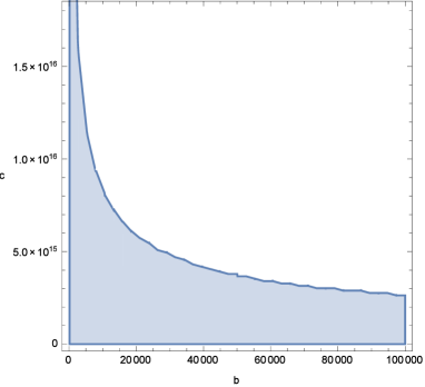
Figure 1: (Colour on-line) The parameter space associated to the parameters b and c, where $0\leq c\leq 2\times 10^{16}m^{-2}$ and $0\leq b\leq 10^{5}$.

III.2 Weinberg angle data

Here we proceed within the example of the Weinberg angle, a right precise measured quantity. After the spontaneous symmetry breaking, the perturbative spectrum can be straightforwardly read from the quadratic terms. Concerning the gauge fields, the relevant terms come from the covariant derivative $|\bar{D}_{\mu}\bar{\varphi}|^{2}$. Assuming the symmetry breaking along the third isospin component, the right spectrum is reached via the identification

$$\left(\begin{array}[]{c}\bar{Z}_{\mu}\\ \bar{A}_{\mu}\end{array}\right)=\left(\begin{matrix}\cos\theta_{W}&-\sin\theta_{W}\\ \sin\theta_{W}&\cos\theta_{W}\end{matrix}\right)\left(\begin{array}[]{c}\overline{W}_{\mu}^{3}\\ \overline{V}_{\mu}\end{array}\right),$$ (19)

where $\theta_{W}$ is the Weinberg angle, $Z_{\mu}$ is the massive neutral boson and $A_{\mu}$ is the electromagnetic field. From the very definition of the Weinberg angle, it is readily verified that $\tan\theta_{W}=\bar{q}/\bar{g}$, which reads as

$$\tan\theta_{W}=\frac{q_{5}}{g_{5}}\frac{\tilde{G}^{1/2}(\overline{\phi}(\bar{r}))}{G^{1/2}(\overline{\phi}(\bar{r}))}\equiv\mathcal{G}(r).$$ (20)

Now we are in position to use the Weinberg angle value (and its associated error) to constraint the brane thickness and, then, refining a given model. For the argument suppose $\tan\theta_{W}=N\pm\Delta N$. Assuming that the brane core is positioned at $\bar{r}=0$, we shall understand $\mathcal{G}(\overline{r})$ with $\overline{r}\in[r_{-},r_{+}]$ (the extremes of the brane) and $\mathcal{G}(\overline{r})\in[N-\Delta N,N+\Delta N]$ as the mapping

$$\mathcal{G}(r) : \left.\mathbb{R}\rightarrow\mathbb{R}\right.$$

$$\left.r\mapsto\mathcal{G}(r).\right.$$

Giving the fact that the brane thickness shall not be macroscopic (by the reasons previously exposed), it is possible to expand the $\mathcal{G}$ as

$$\mathcal{G}(r_{+})=\mathcal{G}(0)+\frac{d\mathcal{G}(0)}{dr}r_{+}+\frac{1}{2}\frac{d^{2}\mathcal{G}(0)}{dr^{2}}r_{+}^{2}+\cdots.$$ (21)

To fix ideas, we make the first order term equal to zero, as it is for the symmetry condition. After a simple algebra we have the following constraint

$$8\left(\frac{d^{2}\mathcal{G}(0)}{dr^{2}}\right)^{-1}(N-\Delta N-\mathcal{G}(0))\leq\delta^{2}\leq 8\left(\frac{d^{2}\mathcal{G}(0)}{dr^{2}}\right)^{-1}(N+\Delta N-\mathcal{G}(0)).$$ (22)

Hence the brane thickness is constrained in the following context: for a given model, whose dependence on the extra dimension is encoded in Eq. (20), the $\delta^{2}$ value must respect the numerical restriction coming from the Weinberg angle measurement. Obviously the analysis is model dependent, but the point to be stressed is that the above analysis may be used in order to refine the model itself, constraining its otherwise free parameters and enabling, thus, the physical viability of the model. Now let us focusing in another point concerning this reasoning. By implementing the same boundaries as in the previous analysis, it is fairly trivial to see that the following inequalities must be fulfilled

$$\left.(N-\mathcal{G}(0))\leq 2,4\times 10^{-10}\left(\frac{d^{2}\mathcal{G}(0)}{dr^{2}}\right)-\Delta N,\right.$$

$$\left.(N-\mathcal{G}(0))\geq 5\times 10^{-39}\left(\frac{d^{2}\mathcal{G}(0)}{dr^{2}}\right)+\Delta N,\right.$$

therefore

$$\Delta N\left(\frac{d^{2}\mathcal{G}(0)}{dr^{2}}\right)^{-1}\leq 1,2\times 10^{-10}\left(1-\frac{10^{-26}}{484}\right)m^{2}.$$ (23)

Hence, we see that $\frac{d^{2}\mathcal{G}(0)}{dr^{2}}$ must be positive. More precisely, disregarding the $10^{-26}$ term, and evaluating the $\Delta N$ factor (which amounts out to be about $1,2\times 10^{-10}$) we have

$$\frac{d^{2}\mathcal{G}(0)}{dr^{2}}\geq 1,0m^{-2}.$$ (24)

It is interesting to notice, then, that this procedure may also refine the localization mechanism itself, by means of the smearing out functions. In fact, by the identification (20), we have

$$\left(\frac{\widetilde{G}(0)\mid G^{\prime\prime}(0)\mid-\mid\widetilde{G}^{\prime\prime}(0)\mid G(0)}{G^{2}(0)}\right)\geq\frac{g_{5}}{q_{5}}.$$ (25)

For instance, we have found under some assumptions in Noi that $G(\overline{\phi}(r))=\mathrm{sech}^{2k}(2cr)$ in the case of the Gremm Model. Similarly, one could choose $\widetilde{G}(\overline{\phi}(r))=\mathrm{sech}^{2\widetilde{k}}(2cr)$. This would furnishes, for instance, $8c^{2}(k-\widetilde{k})\geq\frac{g_{5}}{q_{5}}$ for $k>\widetilde{k}$ and $c>0$, constraint some otherwise free parameters.

IV Final Remarks

By investigating the data from effective bosonic electroweak sector of the standard model in association to current experimental boundaries related to the brane thickness we were able to indicate useful refinements concerning the modeling of braneworlds. The idea of considering electroweak data with respect to their relation to extra dimensions is not new (see, for instance APP ), but our approach is essentially the use of the data related to the rescaled quantities, instead of analyzing radiative corrections.

By using the Higgs boson mass data we find, in particular, for the so-called Gremm’s model, a region in the parameter space $(b,c)$ which serves as allowed domain to the AdS curvature of the model $bc$. Some similar region was obtained in ult but here we were able to evince, due to the Higgs mass data, another region of the allowed domain. We have also analyzed the possible constraints in the brane thickness with respect to the stringent data coming from Weinberg angle measurements. The procedure is particularly interesting whenever the smearing out functions are in place for the gauge fields localization. Ultimately, this procedure is relevant to constraint background parameters arising from the thick brane modeling in warped spaces.

References

- (1) L. Randall and R. Sundrum, Phys. Rev. Lett. 83, 3370 (1999).
- (2) L. Randall and R. Sundrum, Phys. Rev. Lett. 83, 4690 (1999).
- (3) T. Shiromizu, K. Maeda, and M. Sasaki, Phys. Rev. D 62, 043523 (2000).
- (4) A. N. Aliev and A. E. Gumrukcuoglu, Class. Quant. Grav. 21, 5081 (2004).
- (5) R. Maartens and K. Koyama, Living Rev. Relativity 13, 5 (2010).
- (6) N. Arkani-Hamed and M. Schmaltz, Phys. Rev. D 61, 033005 (2000).
- (7) M. Cvetic and H. H. Soleng, Phys. Rep. 282, 159 (1997); M. Cvetic, S. Griffies and S. -J. Rey, Nucl. Phys. B 381, 301 (1992).
- (8) W. D. Goldberger and M. B. Wise, Phys. Rev. Lett. 83, 4922 (1999).
- (9) K. Skenderis and P. K. Townsend, Phys. Lett. B 468, 46 (1999).
- (10) O. DeWolfe, D. Z. Freedman, S. S. Gubser, and A. Karch, Phys. Rev. D 62, 046008 (2000).
- (11) C. Csaki, J. Erlich, T. J. Hollowood and Y. Shirman , Nucl. Phys. B 581, 309 (2000).
- (12) C. Csaki, J. Erlich, C. Grojean and T. J. Hollowood, Nucl. Phys. B 584, 359 (2000).
- (13) O. DeWolfe and D. Z. Freedman, arXiv:0002226 [hep-th].
- (14) M. Gremm, Phys. Lett B 478, 434 (2000) ; Phys. Rev. D 62, 044017 (2000) .
- (15) M. Giovannini, Phys. Rev. D 64, 064023 (2001); ibid 65, 064008 (2002).
- (16) A. Campos, Phys. Rev. Lett. 88, 141602 (2002).
- (17) D. Bazeia, C. Furtado, A. R. Gomes, JCAP 02, 002 (2004).
- (18) D. Bazeia, A. R. Gomes JHEP 012, 0405 (2004).
- (19) R. Koley and S. Kar, Class. Quantum Grav. 22, 753 (2005).
- (20) A. Melfo, N. Pantoja, and J. D. Tempo, Phys. Rev. D 73, 044033 (2006).
- (21) C. Macesanu, Int. J. Mod. Phys. A 21, 2259 (2006).
- (22) Y. -X. Liu, X. -H. Zhang, L. -D. Zhang, and Y. -S. Duan, JHEP 02, 067 (2008); Y. -X. Liu, L. -D. Zhang, S. -W. Wei, and Y. -S. Duan, JHEP 08, 041 (2008); Y. -X. Liu, L. -D. Zhang, L. -J. Zhang, and Y. -S. Duan, Phys. Rev. D 78, 065025 (2008); Y. -X. Liu, Z. -H. Zhao, S. -W. Wei, and Y. -S. Duan, JCAP 02, 003 (2009).
- (23) A. de Souza Dutra, A. C. Amaro de Faria Jr, and M. Hott, Phys. Rev. D 78, 043256 (2008).
- (24) C. A. S. Almeida, R. Casana, M. M. Ferreira Jr., and A. R. Gomes, Phys. Rev. D 79, 125022 (2009).
- (25) Z-H. Zhao, Yu-Xiao Liu and Hai-Tao Li, Class. Quantum Grav. 27, 185001 (2010).
- (26) A. E.R. Chumbes, M. B. Hott, Phys. Rev. D 81, 045008 (2010).
- (27) A. E. R. Chumbes, A. E. O. Vasquez, M. B. Hott, Phys. Rev. D 83, 105010 (2011).
- (28) R. A. C. Correa, A. de Souza Dutra, M. B. Hott Class. Quant. Grav. 28, 155012 (2011).
- (29) A. Kehagias, K. Tamvakis, Phys. Lett. B 504, 38 (2001).
- (30) B. Bajc and G. Gabadadze, Phys. Lett. B 474, 282 (2000).
- (31) C. Germani, Phys. Rev. D 85, 055025 (2012).
- (32) M. N. Smolyakov, Phys. Rev. D 85, 045036 (2012).
- (33) W.T. Cruz, Aristeu R.P. Lima, C.A.S. Almeida Phys. Rev. D 87, 045018 (2013).
- (34) Zhen-Hua Zhao, Yu-Xiao Liu, Yuan Zhong. Phys. Rev. D 90, 045031 (2014).
- (35) A. E. R. Chumbes, J. M. Hoff da Silva, and M. B. Hott, Phys. Rev. D 85, 085003 (2012).
- (36) J. Schwinger, Phys. Rev. 82, 664 (1951).
- (37) R. Friedberg and T. D. Lee, Phys. Rev. 15, 1694 (1977) ; ibid 16 (1977) 1096; ibid 18, 2623 (1978).
- (38) J. M. Hoff da Silva and Roldao da Rocha, Europhys. Lett. 100, 11001 (2012).
- (39) CMS Collaboration, Phys. Lett. B 716, 30 (2012).
- (40) D. J. Kapner, T. S. Cook, E. G. Adelberger, J. H. Gundlach, B. R. Heckel, C. D. Hoyle, and H. E. Swanson, Phys. Rev. Lett. 98, 021101 (2007).
- (41) T. Appelquist, H.-C. Cheng, B. Dobrescu, Phys. Rev. D 64, 035002 (2001).