Spin Polarisation of $t\bar{t}\gamma\gamma$ production at NLO+PS with GoSam interfaced to MadGraph5_aMC@NLO

Abstract

We present an interface between the multipurpose Monte Carlo tool MadGraph5_aMC@NLO and the automated amplitude generator GoSam. As a first application of this novel framework, we compute the NLO corrections to $pp\to$ $t\bar{t}H$ and $pp\to$ $t\bar{t}\gamma\gamma$ matched to a parton shower. In the phenomenological analyses of these processes, we focus our attention on observables which are sensitive to the polarisation of the top quarks.

1 Introduction

The development of automated tools for precise calculations of total cross sections and differential distributions in high-energy collisions has undergone a dramatic acceleration in the last decade. While Leading-Order (LO) tools, based on automated tree-level calculations, have been available for a long time Stelzer:1994ta ; Kanaki:2000ey ; Mangano:2002ea ; Corcella:2002jc ; Maltoni:2002qb ; Gleisberg:2003xi ; Boos:2004kh ; Pukhov:2004ca ; Alwall:2007st ; Kilian:2007gr ; Cafarella:2007pc , the needs of the experimental analyses at the Large Hadron Collider (LHC) and a deeper understanding of the structure of scattering amplitudes Bern:2007dw ; Britto:2010xq ; Ellis:2011cr at one loop led to the development of several computer frameworks for the automated computation of loop matrix elements Giele:2008bc ; Berger:2008sj ; Cullen:2011ac ; Cascioli:2011va ; Actis:2012qn ; Cullen:2014yla and physical observables at Next-to-leading-Order (NLO) accuracy Gleisberg:2008ta ; Bevilacqua:2011xh ; Hirschi:2011pa ; Badger:2012pg ; Alioli:2010xd ; Bellm:2013lba ; Alwall:2014hca . Moreover, techniques to properly deal with the merging of different multiplicities in the final states and the matching Frixione:2002ik ; Nason:2004rx  to parton shower were successfully developed Hamilton:2012np ; Hoeche:2012yf ; Gehrmann:2012yg ; Frederix:2012ps ; Lonnblad:2012ix and are nowadays available.

Advanced automated calculations have been performed by embedding the codes for generating virtual corrections at NLO precision, the so called One Loop Providers (OLPs), within a Monte Carlo program (MC). The interplay between MCs programs and OLPs is controlled by means of interfaces, which allow the user to get direct access to the main features of the MC code, bypassing the need of knowing the technical details of the OLP, which is ideally an inner engine within the MC generator. Many of such interfaces are based on the standards settled by the Binoth Les Houches Accord (BLHA) Binoth:2010xt ; Alioli:2013nda , which defines specifications of the communication between MCs and OLPs.

The LHC has recently started Run II, collecting data at an energy scale never explored before. Within this activities automated multi-purpose tools for particle collisions simulation are of fundamental importance for comparing theoretical predictions with experimental data, thereby extracting important information about the Standard Model (SM) and exploring all traces of deviations from it. The need for flexible tools which at the same time can provide accurate predictions, both in the SM and Beyond (BSM), may become of primary relevance in the near future. It is therefore important to be able to connect different tools to increase the reliablility of results.

With this goals in mind, we present the interface between the multipurpose NLO Monte Carlo tool MadGraph5_aMC@NLO (MG5_aMC) Alwall:2014hca  and the automated one-loop amplitude generator GoSam Cullen:2014yla . The advantage of this combination is twofold. On the one hand, this tandem allows the user of MG5_aMC to switch between two options of OLPs, namely between the inhouse code MadLoop Hirschi:2011pa fully integrated directly in the MC distribution package, and GoSam. Thus, the user can experience the evaluation of NLO virtual corrections by means of two alternative solutions corresponding to different algorithms and methods of generation and evaluation of Feynman amplitudes. On the other hand, GoSam is interfaced to several MCs codes, like SherpaGleisberg:2008ta , Herwig++Bellm:2013lba , PowhegAlioli:2010xd , beside MG5_aMC, therefore the user of the MCs can explore and compare the different features of the event generators, without being biased by the performances of the OLPs, since they all can be run using GoSam.

As an illustration of the novel framework MG5_aMC + GoSam, we present its application to the NLO corrections to $pp\to$ $t\bar{t}H$, $H\to\gamma\gamma$ and the continuum $pp\to$ $t\bar{t}\gamma\gamma$ matched to a parton shower. The production of a Higgs Boson in association with a pair of top anti-top quarks is an important process to directly study the Yukawa coupling of the Higgs Boson with massive fermions. Such a channel, and its corresponding backgrounds, were recently the subject of detailed studies, both at LO Biswas:2014hwa ; Denner:2014wka ; Santos:2015dja and NLO Kardos:2014pba precision. Very recently, new analyses have appeared which further extend these studies including the decay of the top and anti-top quark into bottom quarks and leptons Denner:2015yca , considering the production of a top-quark pair in conjunction with up to two vector bosons Maltoni:2015ena , and exploring the CP-structure of the top-Higgs coupling Buckley:2015vsa . In the phenomenological analysis contained in this paper, we focus our attention on observables sensible to the polarization of the top quarks, such as angular variables which involve the decay of the top quark.

The paper is organized as follows: in Section 2, after a general introduction to the GoSam and MG5_aMC codes, we will discuss the interface between the two frameworks and its validation. In Section 3, we will present an application of the GoSam+ MG5_aMC interface, namely the study of NLO corrections to $pp\to$ $t\bar{t}H$, $H\to\gamma\gamma$ and $pp\to$ $t\bar{t}\gamma\gamma$ matched to a parton shower. Finally in Section 4, we will draw our conclusions.

2 Computational setup

For the computations contained in this paper, the automated one-loop amplitude generator GoSam has been fully interfaced to the MG5_aMC Monte Carlo framework.

In this section, we briefly review the main characteristics of each of these tools and describe the details of the interface between them, which allows to use one-loop amplitudes generated by GoSam within MG5_aMC. Finally we discuss the validation of the interface by means of a comparison with an independent framework.

2.1 GoSam

The main idea that distinguishes the GoSam framework Cullen:2014yla from other codes for the automated generation of one-loop amplitudes is the combined use of automated diagrammatic generation and algebraic manipulation in $d=4-2\epsilon$ dimensions, thus providing analytic expressions for the integrands, with $d$-dimensional integrand-level reduction techniques, or tensorial reduction. Amplitudes are automatically generated via Feynman diagrams and, according to the reduction algorithm selected by the user, are algebraically manipulated and cast in the most appropriate output Nejad:2013ina ; Nogueira:1991ex ; Vermaseren:2000nd ; Reiter:2009ts ; Cullen:2010jv ; Kuipers:2012rf . The individual program tasks are controlled by means of a python code, while the user only needs to prepare an input card to specify the details of the process to be calculated without worrying about internal details of the code generation.

After the generation of all contributing diagrams, the virtual corrections are evaluated using the integrand reduction via Laurent expansion Mastrolia:2012bu , provided by Ninja vanDeurzen:2013saa ; Peraro:2014cba , or the $d$-dimensional integrand-level reduction method Ossola:2006us ; Ellis:2008ir ; Mastrolia:2008jb , as implemented in Samurai Mastrolia:2010nb ; vanDeurzen:2013pja . Alternatively, the tensorial decomposition provided by Golem95C Binoth:2008uq ; Heinrich:2010ax ; Cullen:2011kv ; Guillet:2013msa is also available. The scalar loop integrals can be evaluated using Golem95C, OneLOop vanHameren:2010cp , or QCDLoop vanOldenborgh:1990yc ; Ellis:2007qk .

The GoSam framework can be used to generate and evaluate one-loop corrections in both QCD and electroweak theory Chiesa:2015mya . Model files for Beyond Standard Model (BSM) applications generated from a Universal FeynRules Output (UFO) Degrande:2011ua ; Alloul:2013bka or with LanHEP Semenov:2014rea are also supported. A model file which contains the effective Higgs-gluon couplings that arise in the infinite top-mass limit is also available in the current distribution and it was successfully used to compute the virtual corrections for the production of a Higgs boson in association with 2 and 3 jets vanDeurzen:2013rv ; Cullen:2013saa .

The computation of physical observables at NLO accuracy, such as cross sections and differential distributions, requires to combine the one-loop results for the virtual amplitudes obtained with GoSam, with other parts of the calculations, namely the computation of the real emission contributions and of the subtraction terms, needed to control the cancellation of IR singularities. In some of the earlier calculations performed with GoSam Greiner:2012im ; Cullen:2012eh ; Gehrmann:2013aga ; Gehrmann:2013bga ; Greiner:2013gca , the problem was solved by means of an ad hoc adaptation of the MadDipole-Madgraph4-MadEvent framework Stelzer:1994ta ; Frederix:2008hu ; Frederix:2010cj ; Alwall:2007st .

Far more efficiently, this task can be performed by embedding the calculation of virtual corrections within a multipurpose Monte Carlo program (MC), that can also provide the phase-space integration, which is what is pursued in this work. In this case, the MC takes control over the different stages of the calculation, in particular the phase space integration and the event generation, and calls GoSam at runtime to obtain the corresponding value of the one-loop amplitude at the given phase space points. This approach has the great advantage of making available to the user all the advanced features that the MC generator provides, for example to allow for parton showering, further decays of the final-state hard particles retaining spin correlation and merging of different final state multiplicities.

While in the present paper we will focus on the interface between GoSam and MG5_aMC, it is worth mentioning that a number of phenomenological results can be found in the literature which were obtained by combining GoSam with other MC programs, in particular with Sherpa Gleisberg:2008ta ; Hoeche:2013mua ; vanDeurzen:2013xla ; Heinrich:2013qaa ; Greiner:2015jha , Herwig++ Bellm:2013lba ; Butterworth:2014efa , and Powheg Alioli:2010xd ; Luisoni:2013cuh ; Luisoni:2015mpa .

2.2 MadGraph5_aMC@NLO

The MG5_aMC framework Alwall:2014hca  has been developed to be able to generate events and compute differential cross sections with a high-level of automation. The central idea behind the code is that the structure of cross sections is essentially independent of the process under consideration. Therefore, once this structure has been set up, any cross section can be computed within the framework. For example, even though the matrix elements are process and theory dependent, they can be computed from a very limited set of instructions based on the Feynman rules.

The core of the MG5_aMC framework is based on tree-level amplitude generation, since in this code the matrix elements used in both LO and NLO computations are constructed from tree-level Feynman diagrams. The generation of these amplitudes is based on three elements which are key to taming the complexity of the computation as the number of external particles increases: colour decomposition, helicity amplitudes and recycling of identical substructures between diagrams. The internal algorithms used have been described extensively in Ref. Alwall:2011uj and Ref. Hirschi:2011pa ; Ossola:2006us ; Ossola:2007ax ; Ossola:2008xq ; Cascioli:2011va ; Alwall:2014hca for the generation of tree-level and one-loop matrix elements, respectively.

Beyond the lowest order in perturbation theory, intermediate contributions to the computation of (differential) cross sections are plagued by divergences. In particular the soft/collinear divergences in the numerical phase-space integration over the real-emission (Bremstrahlung) corrections are non-trivial to deal with. In MG5_aMC, the FKS subtraction method Frixione:1995ms ; Frederix:2009yq is used to factor out the singularities in order to cancel them analytically with singularities present in the virtual corrections. The FKS subtraction is based on partitioning the phase-space, in which each phase-space region has at most one collinear and one soft singularity. These singularities are subtracted before performing the numerical phase-space integration by using a straight-forward plus-description. The subtraction terms have been integrated analytically, using dimensional regularisation, once and for all, resulting in explicit poles in $1/\epsilon$ and $1/\epsilon^{2}$, which cancel similar poles in the virtual corrections and the PDFs.

Independently of which code one uses for the computation of the virtual corrections, for example MadLoop Hirschi:2011pa or GoSam Cullen:2014yla , optimisations in the phase-space integration of these contributions are used, as described in Ref. Alwall:2014hca . That is, during the phase-space integration an approximation of the virtual corrections based on the born matrix elements is created dynamically. These approximate virtual matrix elements are very fast to evaluate and can therefore be efficiently integrated numerically with high statistics. The small difference between the approximate and the exact virtual corrections is relatively slow to evaluate for a given phase-space point, but given that this is a very small contribution to the final result, the requirement on the relative precision with which it needs to be computed can be relaxed. Therefore, using low statistics for this complicated contribution suffices, greatly reducing the overall computational time.

To match the short-distance matrix elements to a parton shower, the framework of MG5_aMC employs the MC@NLO technique Frixione:2002ik available for Pythia 6 Sjostrand:2006za , Herwig 6 Corcella:2000bw , Pythia 8 Sjostrand:2014zea  and Herwig++ Bahr:2008pv . In this method, the possible double counting between the NLO corrections and the parton shower is accounted for by explicitly subtracting the parton shower approximation for the emission of a hard parton from the real-emission contributions, and the parton shower approximation of a non-emitting parton from the virtual corrections. To consistently merge various multiplicities at NLO accuracy and match them to the parton shower, the FxFx merging method Frederix:2012ps  is available.

2.3 Interface

The interface between GoSam and MG5_aMC is based on the standards of the first BLHA defined in Binoth:2010xt . When running the MG5_aMC interactive session, the command

$ set OLP GoSam

changes the employed OLP from its default MadLoop to GoSam. Alternatively, the file

input/mg5_configuration.txt

can be directly edited to include the line OLP = GoSam.

The BLHA order and contract file system allows for a basic communication between the two codes to exchange the most fundamental information about the number and type of subprocesses, the powers of the couplings involved in the specific process, the schemes in which the computation should be performed and also the value of parameters like masses and widths. For static parameters, which do not change at each phase space point, but stay constant during the MC integration and event generation, the information is passed via a SUSY Les Houches Accord (SLHA) parameter file. This is created by MG5_aMC and read by GoSam. The path to this SLHA file is specified in the order file with the key word ModelFile. An example generated for the computation of $t\bar{t}\gamma\gamma$ is shown in Figure 1. For parameters which instead may change at each phase space point, the BLHA 1 interface defines an array to pass the numerical value of dynamical variables. The definition and order of the parameters passed through this array is set in the order file using the keyword Parameters. Although in principle extendible to up to ten parameters, at present only the first entry is used, to communicate the value of $\alpha_{S}$.

 

   

 #OLE_order written by MadGraph5_aMC@NLO 

  

 MatrixElementSquareType CHaveraged 

 CorrectionType          QCD 

 IRregularisation        CDR 

 AlphasPower             2 

 AlphaPower              2 

 NJetSymmetrizeFinal     Yes 

 ModelFile               ./param_card.dat 

 Parameters              alpha_s 

  

  

 # process 

 21 21 -> 22 22 6 -6 

 2 -2 -> 22 22 6 -6 

 1 -1 -> 22 22 6 -6 

 -2 2 -> 22 22 6 -6 

 -1 1 -> 22 22 6 -6 

   

 

 

   

 # vim: syntax=olp 

 #@OLP GoSam 2.0.0 

 #@IgnoreUnknown True 

 #@IgnoreCase False 

 #@SyntaxExtensions 

 MatrixElementSquareType CHaveraged | OK 

 CorrectionType QCD | OK 

 IRregularisation CDR | OK 

 AlphasPower 2 | OK 

 AlphaPower 2 | OK 

 NJetSymmetrizeFinal Yes | OK #Ignored by OLP 

 ModelFile ./param_card.dat | OK 

 Parameters alpha_s | OK 

 21 21 -> 22 22 6 -6 | 1 2 

 2 -2 -> 22 22 6 -6 | 1 0 

 1 -1 -> 22 22 6 -6 | 1 3 

 -2 2 -> 22 22 6 -6 | 1 1 

 -1 1 -> 22 22 6 -6 | 1 4 

   

 

Figure 1: Example of order file (above) and contract file (below).

Further customization of the one-loop amplitudes which need to be generated can be achieved by editing a separate input file for GoSam. In the file gosam.rc, additional information can be specified, i.e. the model, the particle content of the loop diagrams, and the number of active flavours. Here it is also possible to define ad hoc filters to remove unwanted diagrams or loop contributions which are known to be negligible or vanishing, which may however, if kept in the calculation, introduce numerical instabilities or slow down the evaluation. Some settings are present by default, but many more can be introduced by the user. We refer to the Appendix for a more extensive list of possible options. The GoSam input file needs to be edited by hand and can be found at

Template/loop_material/OLP_specifics/GoSam/gosam.rc,

in the MG5_aMC repository, or at

OLP_virtuals/gosam.rc,

in the folder that is generated by MG5_aMC automatically when a new process is started. After the input file is ready, any NLO process can be generated following the general MG5_aMC procedure.

The interface between MG5_aMC and GoSam is available starting from MG5_aMC version 2.3.2.2. The two codes can be downloaded from the following URL:

• MG5_aMC: http://amcatnlo.web.cern.ch/amcatnlo/

• GoSam: http://gosam.hepforge.org/

2.4 NLO predictions and validation

To validate the interface, and consequently the results we present in Section 3, several cross checks were performed. The loop amplitudes of GoSam and MadLoop were compared for single phase space points and also at the level of the total cross section for a number of different processes, as presented in a dedicated table in hansthesis . Furthermore, for $pp\rightarrow t\bar{t}\gamma\gamma$, a fully independent check was also performed by computing the same cross section using GoSam interfaced to Sherpa. The comparison between the results obtained with MG5_aMC+GoSam, Sherpa+GoSam, and MG5_aMC+MadLoop is presented Table 1, where we report the total integrated cross sections for LO and NLO at a center-of-mass energy $\sqrt{s}=8$ TeV.

—$\sigma_{t\bar{t}\gamma\gamma}$, $\sqrt{s}=8$ TeV	MG5_aMC + MadLoop	MG5_aMC + GoSam	Sherpa+GoSam
— LO [pb]	$1.0241\pm 5.50\cdot 10^{-4}$		$1.0246\pm 3.51\cdot 10^{-4}$
— NLO [pb]	$1.3507\pm 5.85\cdot 10^{-3}$	$1.3432\pm 5.16\cdot 10^{-3}$	$1.3593\pm 1.80\cdot 10^{-3}$

Table 1: Total cross sections in picobarns, at center-of-mass energy $\sqrt{s}=8$ TeV, for combinations of MCs and OLPs, at LO and NLO.

Figure 2: Transverse momentum of the top quark in $pp\to t\bar{t}\gamma\gamma$ for the LHC at 8 TeV: LO and NLO distributions obtained with GoSam+MG5_aMC (upper plot) and NLO comparison between GoSam+MG5_aMC and GoSam+Sherpa (lower plot).

Figure 3: Photon pair invariant mass distribution in $pp\to t\bar{t}\gamma\gamma$ for the LHC at 8 TeV: LO and NLO distributions obtained with GoSam+MG5_aMC (upper plot) and NLO comparison between GoSam+MG5_aMC and GoSam+Sherpa (lower plot).

The results shown in this and the following sections are computed using the following setup. The mass of the Higgs was set to $m_{H}=125$ GeV, the mass of the top quark to $m_{t}=173.2$ GeV. We work in the $N_{f}=5$ model. The value of the electroweak coupling is set to its low energy limit $\alpha_{EW}^{-1}=137.0$. The mass of the $Z$ boson was set to $m_{Z}=91.1876$ GeV and the value of the Fermi constant to $G_{F}=1.16639\cdot 10^{-5}$ GeV^-2, which fixes the electroweak scheme. For the photons, we used the isolation procedure introduced by Frixione Frixione:1998jh  with minimal transverse momentum $p_{\gamma T\text{min}}=20$ GeV, radius of isolation $R_{\gamma}<0.4$ and Frixione parameters $n=1.0$ and $\epsilon_{\gamma}=1.0$. Furthermore, we applied an isolation radius between the two photons $R_{\gamma\gamma}=0.4$. In leading order calculations, we used the PDF set cteq6L1 Pumplin:2002vw . At next-to-leading order, we instead used the PDF set CT10. The renormalisation and factorisation scales are set to $\mu_{R}=\mu_{F}=\mu_{0}$ with

$$\mu_{0}=\frac{\hat{H}_{T}}{2}=\frac{1}{2}\left(\sum_{\text{final state i}}m_{T,i}\right)$$ (1)

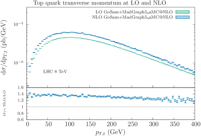
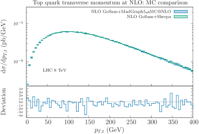
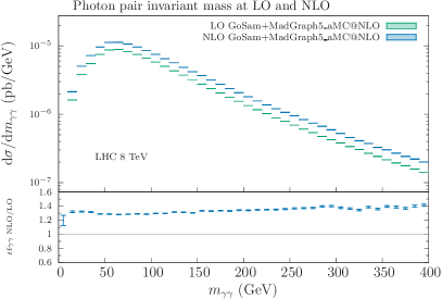
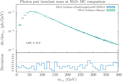
In Figure 2, on the left, we compare LO and NLO predictions for the transverse momentum of the top quark obtained with GoSam+MG5_aMC, while on the right we compare the same NLO predictions with results obtained using GoSam+Sherpa. In Figure 3 we do the same for the photon pair invariant mass. All predictions are computed for a center of mass energy of 8 TeV.

3 Results

In this section we present results at NLO+PS level for the LHC at 13 TeV and compare the background process $t\bar{t}\gamma\gamma$, where the photons are directly radiated from the quarks, with the signal process $t\bar{t}H$ in which the Higgs boson decays to two photons. We will refer to the latter simply as “$t\bar{t}H$”; it should be understood that we consider only the process with the photonic Higgs decay $t\bar{t}H$, $H\rightarrow\gamma\gamma$. As a reference, we also include results for the total cross sections and a selection of distributions obtained at 8 TeV.

The study is performed using NLO predictions for $t\bar{t}H$ and continuum $t\bar{t}\gamma\gamma$ production. The top and anti-top quarks are subsequently decayed semi-leptonically $t\to W^{+}(\to\,\bar{l}\,\nu_{l})b$, $\bar{t}\to\,W^{-}(\to\,l,\bar{\nu}_{l})\bar{b}$ with MadSpin Frixione:2007zp ; Artoisenet:2012st , taking into account spin correlation effects, and then showered and hadronised by means of Pythia 8.2, using its default parameters, but with underlying event turned off. The short-distance events were generated and compared with two slightly different sets of cuts in order to verify that they had no impact on the results at the level of the analysis. Apart from the kinematical requirements on the reconstructed objects, which we will describe below, we use identical model parameters, renormalisation and factorisation scales, PDFs and photon isolation as described in Section 2.4.

Note that for the background process we neglect effects of photon bremsstrahlung from the charged top decay products, which can at least partially be reduced by applying proper kinematical cuts. For the spin correlation observables, on which we will focus our attention in the last part of this section, a LO study Biswas:2014hwa showed that the impact of neglecting these contributions is present but not dramatic.

The analysis cuts are designed to increase the signal over the background, but are by no means optimised to maximise the enhancement. The two photons from the Higgs decay (or the two hard photons in the $t\bar{t}\gamma\gamma$ process) are required to be isolated and fulfill

$$p_{T,\gamma}~{}>~{}20~{}\mathrm{GeV},\quad|\eta_{\gamma}|~{}<~{}2.5,$$ (2)

$$123~{}\mathrm{GeV}~{}<~{}m_{\gamma\gamma}~{}<~{}129~{}\mathrm{GeV}\,,$$

where the invariant mass requirement selects a window around the Higgs boson mass, which reduces the background significantly without altering the signal strength. Furthermore, we require the events to have two oppositely charged leptons and two b-jets coming from the top and anti-top decays. The leptons are selected requiring

$$p_{T,l^{\pm}}~{}>~{}10~{}\mathrm{GeV},\quad|\eta_{l^{\pm}}|~{}<~{}2.7\,.$$ (3)

The b-jets are defined to be jets containing at least one lowest lying B meson. The jets themselves are defined by clustering all stable hadrons and photons, but excluding the two photons selected using Eq. (2), using the anti-$k_{T}$ algortithm as implemented in the code FastJet Cacciari:2005hq ; Cacciari:2008gp ; Cacciari:2011ma , with

$$\Delta R=0.4,\quad p_{T,j}~{}>~{}20~{}\mathrm{GeV},\quad|\eta_{j}|~{}<~{}4.7\,.$$ (4)

We use MC truth information to select the photons from the Higgs decay (signal) or hard events (background) as well as the leptons and b-jets coming from the top and anti-top decays. As reconstructed (anti-)top quark, we use the four-momentum of the (anti-)top quark just before it decays, as provided in the Pythia 8 event record. In the presence of these analysis cuts, we obtain the cross-sections reported in Table 2.

— $\sqrt{s}=8$ TeV	$pp\rightarrow t\bar{t}H$, $H\rightarrow\gamma\gamma$	$pp\rightarrow t\bar{t}\gamma\gamma$
— LO [pb]	$2.90(1)\cdot 10^{-7}~{}{}^{+30\%}_{-21\%}~{}{}^{+14\%}_{-15\%}$	$0.544(1)\cdot 10^{-7}~{}{}^{+27\%}_{-20\%}~{}{}^{+14\%}_{-17\%}$
— NLO [pb]	$3.71(1)\cdot 10^{-7}~{}{}^{+4\%}_{-8\%}~{}{}^{+15\%}_{-16\%}$	$0.770(5)\cdot 10^{-7}~{}{}^{+8\%}_{-9\%}~{}{}^{+13\%}_{-17\%}$
— K-factor	$1.28(1)$	$1.42(1)$
— $\sqrt{s}=13$ TeV	$pp\rightarrow t\bar{t}H$, $H\rightarrow\gamma\gamma$	$pp\rightarrow t\bar{t}\gamma\gamma$
— LO [pb]	$8.84(2)\cdot 10^{-7}~{}{}^{+27\%}_{-20\%}~{}{}^{+10\%}_{-11\%}$	$1.442(2)\cdot 10^{-7}~{}{}^{+25\%}_{-18\%}~{}{}^{+10\%}_{-12\%}$
— NLO [pb]	$11.77(5)\cdot 10^{-7}~{}{}^{+6\%}_{-8\%}~{}{}^{+11\%}_{-12\%}$	$2.175(7)\cdot 10^{-7}~{}{}^{+10\%}_{-10\%}~{}{}^{+10\%}_{-11\%}$
— K-factor	$1.33(1)$	$1.51(1)$
NLO Ratio 13TeV/8TeV	$3.17(2)$	$2.82(2)$

Table 2: Cross sections in picobarns, at a center-of-mass energy of $\sqrt{s}=8$ TeV (upper part) and $\sqrt{s}=13$ TeV (lower part) in the presence of the analysis cuts described in the text. The two sets of uncertainties following the cross section correspond to the scale and PDF variations respectively. We also report the ratio between the cross sections at the two center of mass energies.

In the next section we focus our attention on some relevant observables related to a single particle, whereas in Section 3.2 we will concentrate on observables which can directly probe correlation effects due to the top quark polarisation.

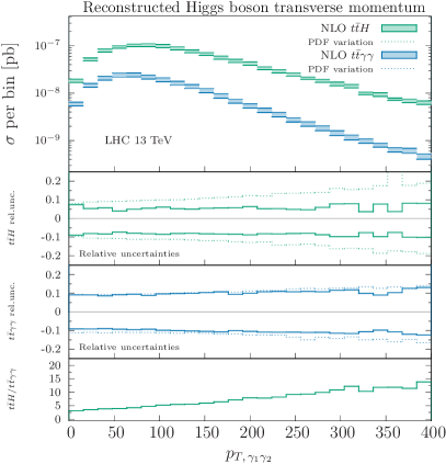
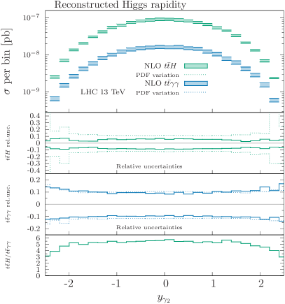
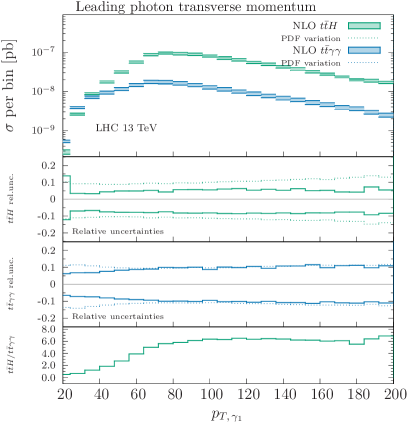
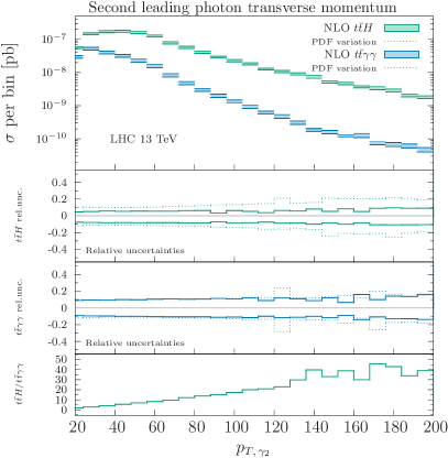
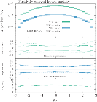
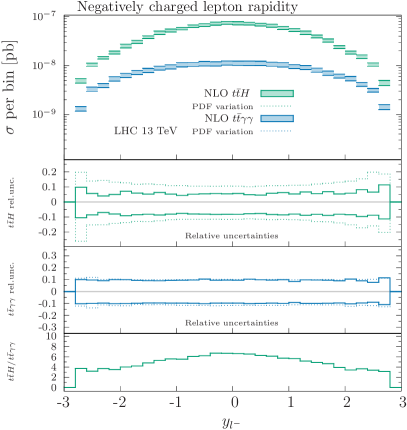
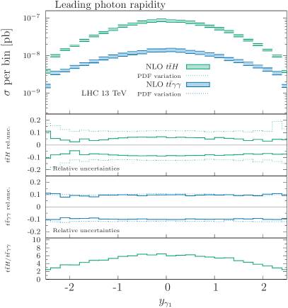
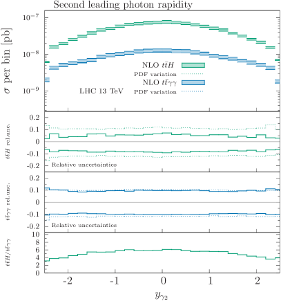
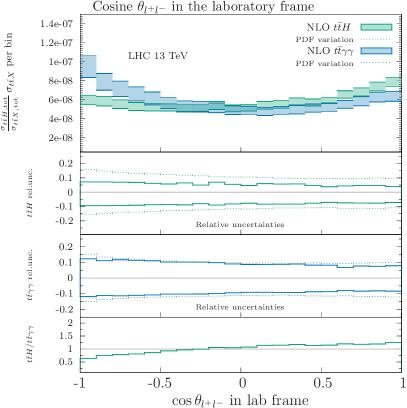
In what follows and unless specified otherwise, the plots will always consist of four distributions. The top curves show the differential cross sections for a given observable and for both the signal and the background process. The two middle insets display the relative uncertainty of the $t\bar{t}H$ and $t\bar{t}\gamma\gamma$ predictions respectively. The scale dependence (transparent band) is estimated by taking the envelope of the nine predictions obtained by the separate variation of renormalisation and factorisation scales by factors of 0.5 and 2 around the central scale $\mu_{0}$ defined in Equation (1). For estimating the PDF uncertainty (dotted lines), we use the Hessian method. Finally, the bottom inset highlights the differential signal-to-background ratio.

3.1 Single particle observables

We start comparing the transverse momentum distribution of the reconstructed top and anti-top quarks, which is shown in Figures 4 and 5, for a center of mass energy of 8 TeV and 13 TeV respectively.

Figure 4: Transverse momentum distribution of the top quark (above) and anti-top quark (below) at 8 TeV.

Figure 5: Transverse momentum distribution of the top quark (above) and anti-top quark (below) at 13 TeV.

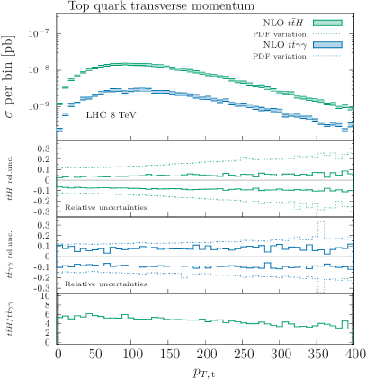
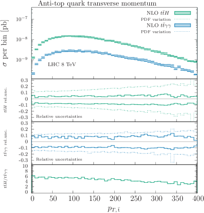
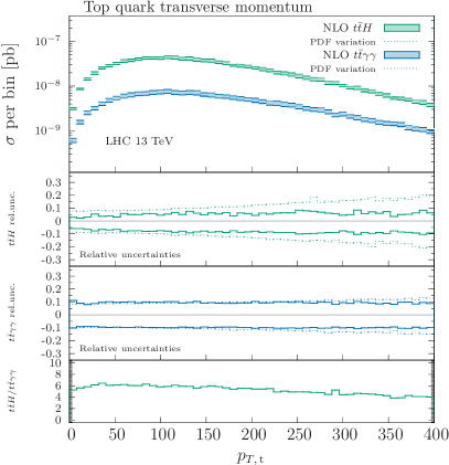
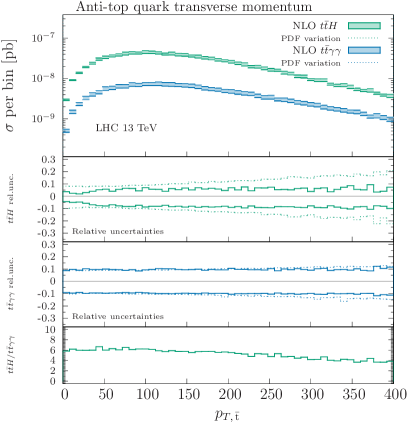
For either the signal or background process, the shapes of the top and anti-top quark $p_{T}$ distributions are very similar, as expected, and therefore the same is true for the signal-to-background ratio. In both cases, it reaches a maximum between $50$ and $100~{}{{\mathrm{GeV}}}$ and than decreases slightly in the high transverse momentum tail. Increasing the center-of-mass energy from 8 to 13 TeV does not lead to significant changes. Since this is true also for the other distributions that we studied, in the following we will only report and comment on the 13 TeV scenario.

It is worth noting, by looking at Figure 5, that the uncertainty due to the PDF variation is larger in $t\bar{t}H$, due to the dominant gluon-channel production, and is increasing for larger transverse momenta. At $p_{T}\approx 400~{}{{\mathrm{GeV}}}$ the PDF uncertainty for $t\bar{t}H$ is around 20%, whereas it stays below 15% for $t\bar{t}\gamma\gamma$.

Figure 6 shows the transverse momentum and the rapidity of the photon pair, which for the signal process corresponds to the one of the reconstructed Higgs boson. Since in $t\bar{t}\gamma\gamma$ the photon pair does not originate from a massive particle decay, its transverse momentum is softer and the spectrum falls off faster for large $p_{T}$. The signal-to-background rapidity curve shows that photons coming from the decay of the Higgs boson are generally produced more centrally. This is not surprising given that such a decay does not feature a collinear enhancement, contrary to the case of $t\bar{t}\gamma\gamma$.

Figure 6: Transverse momentum (top) and rapidity (bottom) distributions of the reconstructed Higgs boson.

The transverse momentum distribution for the single photons (ordered according to their $p_{T}$) is shown in Figure 7. The shoulder in the $t\bar{t}H$ signal distribution stemming from the presence of the Higgs boson resonance is also visible in the background shape, albeit less pronounced, given the invariant mass cut on the photon pair. As expected, the shoulder is shifted towards lower transverse momenta for the case of $t\bar{t}\gamma\gamma$, because of the initial state collinear enhancement.

Figure 7: Transverse momentum distribution of the leading (top) and second leading photon (bottom).

It is particularly interesting to compare the rapidities of the top and anti-top quarks (Figure 8) and of their decay products. This highlights the well known difference between the broadness of the respective top and anti-top quark rapidity distribution and it can be used to improve on background discrimination. This difference is known as the charge asymmetry and is usually quantified by the following observable:

$$A_{\mathrm{t\bar{t}}}^{\mathrm{C}}=\frac{\sigma\left(\Delta|y|>0\right)-\sigma\left(\Delta|y|<0\right)}{\sigma\left(\Delta|y|>0\right)+\sigma\left(\Delta|y|<0\right)}\,,$$ (5)

where $\Delta|y|=|y_{\mathrm{t}}|-|y_{\bar{\mathrm{t}}}|$. This observable has been measured at the LHC by both the ATLAS ATLAS:2012an ; Aad:2013cea and the CMS Chatrchyan:2011hk ; Khachatryan:2015oga ; CMS:2014sfa collaboration in the context of top-quark studies.

Figure 8: Rapidity distribution of the top quark (top) and anti-top quark (bottom).

Figure 9: Upper plot: the rapidity distribution comparison between the top and anti-top quark for $t\bar{t}H$ (above) and $t\bar{t}\gamma\gamma$ (below). Lower plot: normalized top (above) and anti-top (below) rapidity distribution for signal and background.

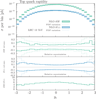
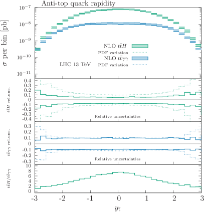
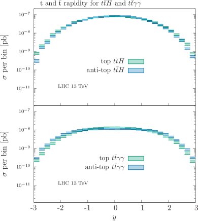
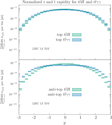
For top-pair production at the LHC $A_{\mathrm{t\bar{t}}}^{\mathrm{C}}$ is positive, i.e. top quarks are produced at larger rapidities compared to anti-top quarks Kuhn:1998kw . It is however known that the presence of a photon reverses the sign of $A_{\mathrm{t\bar{t}}}^{\mathrm{C}}$ already at tree-level Aguilar-Saavedra:2014vta . This change in the rapidity distributions of the top and anti-top quarks, due to additional photon radiation, can clearly be seen in the plots of Figure 9, which compare $y_{\mathrm{t}}$ and $y_{\mathrm{\bar{t}}}$ individually for $t\bar{t}H$ and $t\bar{t}\gamma\gamma$. In the signal process the additional presence of a Higgs boson in the final state does not change the qualitative result, as compared to simple $t\bar{t}$-production. This can be seen in the upper portion of the top plot in Figure 9, which shows that top quarks are produced at slightly higher rapidities, as compared to anti-tops, which are more central, leading to a positive $A_{\mathrm{t\bar{t}}}^{\mathrm{C}}$. In the lower left plot, instead, the effect is reversed. The presence of the additional photons causes the top quarks to be more central compared to the anti-tops.

This effect is even more visible when comparing directly the distributions for $t\bar{t}H$ with the ones for $t\bar{t}\gamma\gamma$. To better appreciate the change in the shape, which is only marginally visible in Figure 8, we plot the same distribution normalized to the inclusive $t\bar{t}H$ cross section on the lower part of Figure 9. From the upper plot it becomes clear that the top quark rapidities have very similar shape in both the signal and the background process, although in the latter the tops are produced at slightly higher rapidities. This means that despite the top being produced at higher rapidities as compared to the anti-top in $t\bar{t}H$, overall, they are still slightly more central than in $t\bar{t}\gamma\gamma$. The opposite is true for the anti-top quark rapidity, and, therefore, the difference is even more visible in the lower plot of Figure 9.

Figure 10: Rapidity distribution distribution of the b-jet (top) and anti-b jet (bottom) produced in the decay of the top and anti-top quark respectively.

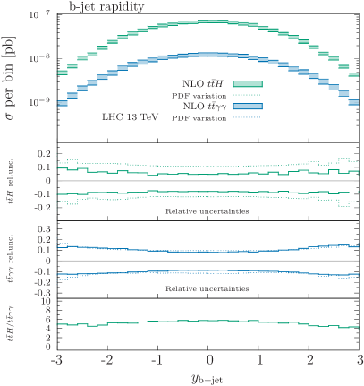
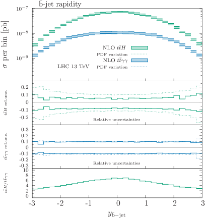
Analogous conclusions can be derived by looking at the rapidities of the top decay products. They are shown in Figure 10 and 11, where the rapidities of the $b$- and $\bar{b}$-jets and the charged leptons are shown respectively.

Figure 11: Rapidity distribution of the lepton (top) and anti-lepton (bottom) produced in the decay of the top and anti-top quark respectively.

In Figure 12 we compare the rapidities of the leading and second leading photon. Not surprisingly, the photon coming form the Higgs boson decay are produced more centrally as compared to the ones radiated from the partons.

Figure 12: Rapidity distribution of the leading (top) and second leading photon (bottom).

3.2 Spin polarisation observables

In this section we focus on observables that allow for investigating polarisation effects of the top and anti-top quarks as well as in their decay products. This can be done by studying angular variables which involve the decay products of the top and anti-top quarks; both top quarks are considered to decay semileptonically (same as in the previous section). We stress that a similar analysis was already performed at LO in Ref. Biswas:2014hwa .

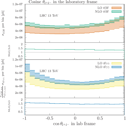
Typically, for hadronic $t\bar{t}$-production, very specific kinematic frames are defined Bernreuther:2001rq ; Bernreuther:2004jv ; Bernreuther:2010ny . In the following we will consider the three-dimensional opening angle $\theta_{ll}$ between the leptonic decay products of the top ($l^{+}$) and anti-top quarks ($l^{-}$), defined in three different frames. The most straightforward possibility is to define $\theta_{ll}$ in the laboratory frame (referred to as lab-frame in the following). The results for this case are shown in Figure 13. The definition of two other frames, introduced for the first time in Bernreuther:2004jv , became customary in polarisation studies, since they capture particularly well spin correlation effects.

Figure 13: $\cos\theta_{ll}$ distribution for the signal ($t\bar{t}H$) and background ($t\bar{t}\gamma\gamma$) processes in the laboratory frame. The exact definition of the angle $\theta$ is given in the text. The $t\bar{t}\gamma\gamma$ prediction is normalized to the $t\bar{t}H$ inclusive cross-section. In the upper plot, we compare LO with NLO predictions and show their K-factor separately for $t\bar{t}H$ and $t\bar{t}\gamma\gamma$ in bottom insets. In the lower plot, we show NLO relative uncertainties with the signal-to-background ratio as the last bottom inset.

For these particular frames, we define $\theta_{ll}$ to be the angle between the direction of flight of $l^{+}$, measured in frame where the top quark is at rest, and the direction of flight of $l^{-}$, measured in the frame where the anti-top quark is at rest. Since two rest frames are involved in this definition, a common initial frame needs to be specified, from which the (rotation-free) Lorentz boost can be applied in order to transform the system to the $t$ and $\bar{t}$ rest frames. We choose two possible starting points, which we label as frame-1 and frame-2, defined as follows:

• frame-1: the Lorentz boosts to bring $t$ and $\bar{t}$ separately at rest are defined with respect to the $t\bar{t}$-pair center-of-mass frame,

• frame-2: the Lorentz boosts to bring $t$ and $\bar{t}$ separately at rest are defined with respect to the lab-frame.

These two frames are designed to be maximally sensitive to the different polarisation structures of the top-pair in the final state. Furthermore, as already demonstrated at LO Biswas:2014hwa , considering the spin information in the decay of the top and anti-top quark is crucial to disentangle the two different final states, which otherwise look identical, being characterized by a completely flat distribution in both cases.

Figure 14: Same as Figure 13, but for reference frame-1.

Figure 15: Same as Figure 13, but for reference frame-2.

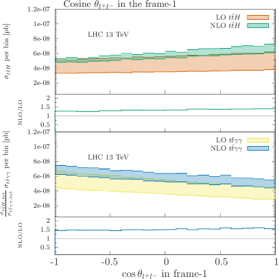
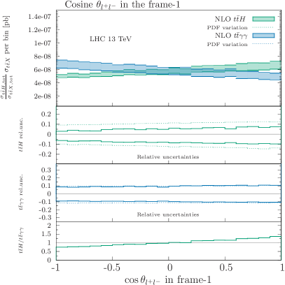
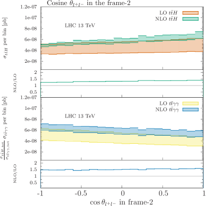
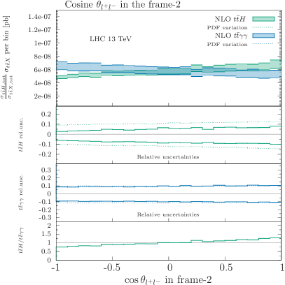
In Figure 13 we show the behaviour of $\cos\theta_{ll}$ in the lab-frame. To highlight shape differences, the background predictions have been normalized to the inclusive $t\bar{t}H$ cross section. The upper portions of Figures 13-15 presents the comparison of the LO and NLO predictions for $t\bar{t}H$ and $t\bar{t}\gamma\gamma$ separately and shows their respective differential K-factors. The histograms in the lower portion of the Figures compare results for the signal and background processes, with their ratio and respective relative uncertainty in the bottom insets.

This is to be compared with the plots in Figures 14-15, where the same observable is shown in frame-1 and frame-2. In the two latter frames a difference in the sign of the slope emerges, while in the lab frame, despite a clear difference in the slopes, the curves have an analogous trend. By comparing the two ratio plots at the bottom of the right plots in Figures 14 and 15, we conclude that the frame-1 offers the best signal-to-background ratio. It is also worth stressing that, while in the lab frame the K-factors tend to decrease slightly when $\cos\theta_{ll}\to 1$, in frame-1 and frame-2, the NLO corrections feature an almost perfectly flat K-factor which agrees with the inclusive cross section K-factor reported in Table 1. A comparison of the LO and NLO predictions reveals the anticipated reduction of the scale uncertainties.

Let us finally remark that the results shown here for the background, only consider photon radiation from the initial state and from the top and anti-top quark, but not from their decay products. This is opposite to the case of the signal, where photons always originate from the decay of the Higgs boson. By considering more general cases and using top tagging techniques without relying on MC truth is expected to decrease the purity of the signal. A more quantitative analysis of these effects is beyond the scope of the present work.

4 Conclusions

The event generator MG5_aMC and the one-loop amplitudes provider GoSam have been interfaced to provide the user with a framework implenting the most advanced techniques for the evaluation of cross sections and differential distributions at next-to-leading order (NLO) accuracy.

In this work, the integration of the two codes has been applied for the first time to the NLO corrections to the production of a Higgs Boson in association with a pair of top-antitop quarks, as well as to the background process where two hard photons are produced directly. We compared several key distributions to disentangle the two processes and focused in particular on observables designed to study spin correlation effects. We found that NLO corrections give a sizable contribution, which however distorts the shape of the distributions only very mildly. Moreover, we observed a clear reduction of the theoretical uncertainties.

The high-level of flexibility and reliability of the joined technologies of the two codes make of the combination of MG5_aMC and GoSam an ideal tool for the high-precision studies and the hunt for deviations from known-physics signals which characterise the Run II programme at the LHC.

Appendix A The GoSam input card

We report here a copy of the default GoSam input card with a brief explanation of the different options. For a more detailed overview we refer to the GoSam papers Cullen:2011ac ; Cullen:2014yla and the GoSam manual which can be found online gosamhome and is continuously updated. The default gosam.rc file is the following:

 

   

 ############################################### 

 # Copy this file to setup.in in order to set 

 # some common options for all examples. 

 ################### 

 # physics options # 

 ################### 

 # Model specs.: 

 model=smdiag_mad 

 model.options=GF: 0.0000116639, mZ: 91.188, 

 mW: 80.419, Nf: 4 

  

 # Parameters set to zero algebraically: 

 zero=me,mmu,mU,mD,mC,mS,wB,wT 

  

 # Symmetries: 

 symmetries=family,generation 

  

 # Filter for scale-less loop integrals: 

 filter.nlo=lambda d: (not (d.isScaleless())) 

  

 ################### 

 # program options # 

 ################### 

 form.bin=tform 

 form.threads=4 

 form.tempdir=/tmp 

 fc.bin=gfortran -O2 

 ############################################### 

   

 

This input file needs to be modified if the computation is performed within the 5-flavour scheme. The b-quark mass can be set algebraically to zero by adding mB to the list zero:

zero=me,mmu,mU,mD,mC,mS,mB,wB,wT.

Furthermore the number of light quarks Nf has to be set equal to 5.

The tag symmetries specifies some further symmetries in the calculation of the amplitudes. The information is used when the list of helicities is generated. Possible options are:

• flavour: does not allow for flavour changing interactions. When this option is set, fermion lines are assumed not to mix.

• family: allows for flavour-changing interactions only within the same family. When this option is set, fermion lines 1-6 are assumed to mix only within families. This means that e.g. a quark line connecting an up with down quark would be considered, while a up-bottom one would not.

• lepton: means for leptons what “flavour” means for quarks.

• generation: means for leptons what “family” means for quarks.

Furthermore it is possible to fix the helicity of particles. This can be done using the command %<n>=<h>, where $<n>$ stands for a PDG number and $<h>$ for an helicity. For example %23=+- specifies the helicity of all $Z$-bosons to be “+” and “-” only (no “0” polarisation).

The filter

filter.nlo=lambda d: (not (d.isScaleless()))

removes possible scaleless loop diagrams which may be generated by QGRAF. Several predefined filters to select only subsets of diagrams exist and can be used in this tag. The full list and some examples can be found in gosamhome .

References

- (1) T. Stelzer and W. Long, Automatic generation of tree level helicity amplitudes, Comput.Phys.Commun. 81 (1994) 357–371, [hep-ph/9401258].
- (2) A. Kanaki and C. G. Papadopoulos, HELAC: A Package to compute electroweak helicity amplitudes, Comput.Phys.Commun. 132 (2000) 306–315, [hep-ph/0002082].
- (3) M. L. Mangano, M. Moretti, F. Piccinini, R. Pittau, and A. D. Polosa, ALPGEN, a generator for hard multiparton processes in hadronic collisions, JHEP 0307 (2003) 001, [hep-ph/0206293].
- (4) G. Corcella, I. Knowles, G. Marchesini, S. Moretti, K. Odagiri, et. al., HERWIG 6.5 release note, hep-ph/0210213.
- (5) F. Maltoni and T. Stelzer, MadEvent: Automatic event generation with MadGraph, JHEP 0302 (2003) 027, [hep-ph/0208156].
- (6) T. Gleisberg, S. Hoeche, F. Krauss, A. Schalicke, S. Schumann, et. al., SHERPA 1. alpha: A Proof of concept version, JHEP 0402 (2004) 056, [hep-ph/0311263].
- (7) CompHEP Collaboration Collaboration, E. Boos et. al., CompHEP 4.4: Automatic computations from Lagrangians to events, Nucl.Instrum.Meth. A534 (2004) 250–259, [hep-ph/0403113].
- (8) A. Pukhov, CalcHEP 2.3: MSSM, structure functions, event generation, batchs, and generation of matrix elements for other packages, hep-ph/0412191.
- (9) J. Alwall, P. Demin, S. de Visscher, R. Frederix, M. Herquet, et. al., MadGraph/MadEvent v4: The New Web Generation, JHEP 0709 (2007) 028, [arXiv:0706.2334].
- (10) W. Kilian, T. Ohl, and J. Reuter, WHIZARD: Simulating Multi-Particle Processes at LHC and ILC, Eur.Phys.J. C71 (2011) 1742, [arXiv:0708.4233].
- (11) A. Cafarella, C. G. Papadopoulos, and M. Worek, Helac-Phegas: A Generator for all parton level processes, Comput.Phys.Commun. 180 (2009) 1941–1955, [arXiv:0710.2427].
- (12) Z. Bern, L. J. Dixon, and D. A. Kosower, On-Shell Methods in Perturbative QCD, Annals Phys. 322 (2007) 1587–1634, [arXiv:0704.2798].
- (13) R. Britto, Loop Amplitudes in Gauge Theories: Modern Analytic Approaches, J.Phys.A A44 (2011) 454006, [arXiv:1012.4493]. 34 pages. Invited review for a special issue of Journal of Physics A devoted to ’Scattering Amplitudes in Gauge Theories’.
- (14) R. K. Ellis, Z. Kunszt, K. Melnikov, and G. Zanderighi, One-loop calculations in quantum field theory: from Feynman diagrams to unitarity cuts, Phys.Rept. 518 (2012) 141–250, [arXiv:1105.4319].
- (15) W. Giele and G. Zanderighi, On the Numerical Evaluation of One-Loop Amplitudes: The Gluonic Case, JHEP 0806 (2008) 038, [arXiv:0805.2152].
- (16) C. Berger, Z. Bern, L. Dixon, F. Febres Cordero, D. Forde, et. al., An Automated Implementation of On-Shell Methods for One-Loop Amplitudes, Phys.Rev. D78 (2008) 036003, [arXiv:0803.4180].
- (17) G. Cullen, N. Greiner, G. Heinrich, G. Luisoni, P. Mastrolia, et. al., Automated One-Loop Calculations with GoSam, Eur.Phys.J. C72 (2012) 1889, [arXiv:1111.2034].
- (18) F. Cascioli, P. Maierhofer, and S. Pozzorini, Scattering Amplitudes with Open Loops, Phys.Rev.Lett. 108 (2012) 111601, [arXiv:1111.5206].
- (19) S. Actis, A. Denner, L. Hofer, A. Scharf, and S. Uccirati, Recursive generation of one-loop amplitudes in the Standard Model, JHEP 1304 (2013) 037, [arXiv:1211.6316].
- (20) G. Cullen, H. van Deurzen, N. Greiner, G. Heinrich, G. Luisoni, et. al., GS-2.0: a tool for automated one-loop calculations within the Standard Model and beyond, Eur.Phys.J. C74 (2014), no. 8 3001, [arXiv:1404.7096].
- (21) T. Gleisberg, S. Hoeche, F. Krauss, M. Schonherr, S. Schumann, et. al., Event generation with SHERPA 1.1, JHEP 0902 (2009) 007, [arXiv:0811.4622].
- (22) G. Bevilacqua, M. Czakon, M. Garzelli, A. van Hameren, A. Kardos, et. al., HELAC-NLO, Comput.Phys.Commun. 184 (2013) 986–997, [arXiv:1110.1499].
- (23) V. Hirschi, R. Frederix, S. Frixione, M. V. Garzelli, F. Maltoni, et. al., Automation of one-loop QCD corrections, JHEP 1105 (2011) 044, [arXiv:1103.0621].
- (24) S. Badger, B. Biedermann, P. Uwer, and V. Yundin, Numerical evaluation of virtual corrections to multi-jet production in massless QCD, Comput.Phys.Commun. 184 (2013) 1981–1998, [arXiv:1209.0100].
- (25) S. Alioli, P. Nason, C. Oleari, and E. Re, A general framework for implementing NLO calculations in shower Monte Carlo programs: the POWHEG BOX, JHEP 1006 (2010) 043, [arXiv:1002.2581].
- (26) J. Bellm, S. Gieseke, D. Grellscheid, A. Papaefstathiou, S. Platzer, et. al., Herwig++ 2.7 Release Note, arXiv:1310.6877.
- (27) J. Alwall, R. Frederix, S. Frixione, V. Hirschi, F. Maltoni, et. al., The automated computation of tree-level and next-to-leading order differential cross sections, and their matching to parton shower simulations, JHEP 1407 (2014) 079, [arXiv:1405.0301].
- (28) S. Frixione and B. R. Webber, Matching NLO QCD computations and parton shower simulations, JHEP 0206 (2002) 029, [hep-ph/0204244].
- (29) P. Nason, A New method for combining NLO QCD with shower Monte Carlo algorithms, JHEP 0411 (2004) 040, [hep-ph/0409146].
- (30) K. Hamilton, P. Nason, and G. Zanderighi, MINLO: Multi-Scale Improved NLO, JHEP 1210 (2012) 155, [arXiv:1206.3572].
- (31) S. Hoeche, F. Krauss, M. Schonherr, and F. Siegert, QCD matrix elements + parton showers: The NLO case, JHEP 1304 (2013) 027, [arXiv:1207.5030].
- (32) T. Gehrmann, S. Hoche, F. Krauss, M. Schonherr, and F. Siegert, NLO QCD matrix elements + parton showers in hadrons, JHEP 01 (2013) 144, [arXiv:1207.5031].
- (33) R. Frederix and S. Frixione, Merging meets matching in MC@NLO, JHEP 1212 (2012) 061, [arXiv:1209.6215].
- (34) L. L nnblad and S. Prestel, Merging Multi-leg NLO Matrix Elements with Parton Showers, JHEP 1303 (2013) 166, [arXiv:1211.7278].
- (35) T. Binoth, F. Boudjema, G. Dissertori, A. Lazopoulos, A. Denner, et. al., A Proposal for a standard interface between Monte Carlo tools and one-loop programs, Comput.Phys.Commun. 181 (2010) 1612–1622, [arXiv:1001.1307].
- (36) S. Alioli, S. Badger, J. Bellm, B. Biedermann, F. Boudjema, et. al., Update of the Binoth Les Houches Accord for a standard interface between Monte Carlo tools and one-loop programs, arXiv:1308.3462.
- (37) S. Biswas, R. Frederix, E. Gabrielli, and B. Mele, Enhancing the signal through top-quark spin polarization effects at the LHC, JHEP 07 (2014) 020, [arXiv:1403.1790].
- (38) A. Denner, R. Feger, and A. Scharf, Irreducible background and interference effects for Higgs-boson production in association with a top-quark pair, JHEP 04 (2015) 008, [arXiv:1412.5290].
- (39) S. P. A. dos Santos et. al., Angular distributions in reconstructed events at the LHC, Phys. Rev. D92 (2015) 034021, [arXiv:1503.0778].
- (40) A. Kardos and Z. Trocsanyi, Hadroproduction of t-anti-t pair with two isolated photons with PowHel, Nucl. Phys. B897 (2015) 717–731, [arXiv:1408.0278].
- (41) A. Denner and R. Feger, NLO QCD corrections to off-shell top-antitop production with leptonic decays in association with a Higgs boson at the LHC, arXiv:1506.0744.
- (42) F. Maltoni, D. Pagani, and I. Tsinikos, Associated production of a top-quark pair with vector bosons at NLO in QCD: impact on searches at the LHC, arXiv:1507.0564.
- (43) M. R. Buckley and D. Goncalves, Boosting the Direct CP Measurement of the Higgs-Top Coupling, arXiv:1507.0792.
- (44) B. C. Nejad, T. Hahn, J. N. Lang, and E. Mirabella, FormCalc 8: Better Algebra and Vectorization, arXiv:1310.0274.
- (45) P. Nogueira, Automatic Feynman graph generation, J.Comput.Phys. 105 (1993) 279–289.
- (46) J. A. M. Vermaseren, New features of FORM, math-ph/0010025.
- (47) T. Reiter, Optimising Code Generation with haggies, Comput.Phys.Commun. 181 (2010) 1301–1331, [arXiv:0907.3714].
- (48) G. Cullen, M. Koch-Janusz, and T. Reiter, Spinney: A Form Library for Helicity Spinors, Comput.Phys.Commun. 182 (2011) 2368–2387, [arXiv:1008.0803].
- (49) J. Kuipers, T. Ueda, J. Vermaseren, and J. Vollinga, FORM version 4.0, Comput.Phys.Commun. 184 (2013) 1453–1467, [arXiv:1203.6543].
- (50) P. Mastrolia, E. Mirabella, and T. Peraro, Integrand reduction of one-loop scattering amplitudes through Laurent series expansion, JHEP 1206 (2012) 095, [arXiv:1203.0291].
- (51) H. van Deurzen, G. Luisoni, P. Mastrolia, E. Mirabella, G. Ossola, et. al., Multi-leg One-loop Massive Amplitudes from Integrand Reduction via Laurent Expansion, JHEP 1403 (2014) 115, [arXiv:1312.6678].
- (52) T. Peraro, Ninja: Automated Integrand Reduction via Laurent Expansion for One-Loop Amplitudes, Comput.Phys.Commun. 185 (2014) 2771–2797, [arXiv:1403.1229].
- (53) G. Ossola, C. G. Papadopoulos, and R. Pittau, Reducing full one-loop amplitudes to scalar integrals at the integrand level, Nucl.Phys. B763 (2007) 147–169, [hep-ph/0609007].
- (54) R. Ellis, W. T. Giele, Z. Kunszt, and K. Melnikov, Masses, fermions and generalized -dimensional unitarity, Nucl.Phys. B822 (2009) 270–282, [arXiv:0806.3467].
- (55) P. Mastrolia, G. Ossola, C. Papadopoulos, and R. Pittau, Optimizing the Reduction of One-Loop Amplitudes, JHEP 0806 (2008) 030, [arXiv:0803.3964].
- (56) P. Mastrolia, G. Ossola, T. Reiter, and F. Tramontano, Scattering AMplitudes from Unitarity-based Reduction Algorithm at the Integrand-level, JHEP 1008 (2010) 080, [arXiv:1006.0710].
- (57) H. van Deurzen, Associated Higgs Production at NLO with GoSam, Acta Phys.Polon. B44 (2013), no. 11 2223–2230.
- (58) T. Binoth, J.-P. Guillet, G. Heinrich, E. Pilon, and T. Reiter, Golem95: A Numerical program to calculate one-loop tensor integrals with up to six external legs, Comput.Phys.Commun. 180 (2009) 2317–2330, [arXiv:0810.0992].
- (59) G. Heinrich, G. Ossola, T. Reiter, and F. Tramontano, Tensorial Reconstruction at the Integrand Level, JHEP 1010 (2010) 105, [arXiv:1008.2441].
- (60) G. Cullen, J. Guillet, G. Heinrich, T. Kleinschmidt, E. Pilon, et. al., Golem95C: A library for one-loop integrals with complex masses, Comput.Phys.Commun. 182 (2011) 2276–2284, [arXiv:1101.5595].
- (61) J. P. Guillet, G. Heinrich, and J. F. von Soden-Fraunhofen, Tools for NLO automation: extension of the golem95C integral library, Comput. Phys. Commun. 185 (2014) 1828–1834, [arXiv:1312.3887].
- (62) A. van Hameren, OneLOop: For the evaluation of one-loop scalar functions, Comput.Phys.Commun. 182 (2011) 2427–2438, [arXiv:1007.4716].
- (63) G. van Oldenborgh, FF: A Package to evaluate one loop Feynman diagrams, Comput.Phys.Commun. 66 (1991) 1–15.
- (64) R. K. Ellis and G. Zanderighi, Scalar one-loop integrals for QCD, JHEP 02 (2008) 002, [arXiv:0712.1851].
- (65) M. Chiesa, N. Greiner, and F. Tramontano, Electroweak corrections for LHC processes, arXiv:1507.0857.
- (66) C. Degrande, C. Duhr, B. Fuks, D. Grellscheid, O. Mattelaer, et. al., UFO - The Universal FeynRules Output, Comput.Phys.Commun. 183 (2012) 1201–1214, [arXiv:1108.2040].
- (67) A. Alloul, N. D. Christensen, C. Degrande, C. Duhr, and B. Fuks, FeynRules 2.0 - A complete toolbox for tree-level phenomenology, Comput.Phys.Commun. 185 (2014) 2250–2300, [arXiv:1310.1921].
- (68) A. Semenov, LanHEP - a package for automatic generation of Feynman rules from the Lagrangian. Updated version 3.2, arXiv:1412.5016.
- (69) H. van Deurzen, N. Greiner, G. Luisoni, P. Mastrolia, E. Mirabella, et. al., NLO QCD corrections to the production of Higgs plus two jets at the LHC, Phys.Lett. B721 (2013) 74–81, [arXiv:1301.0493].
- (70) G. Cullen, H. van Deurzen, N. Greiner, G. Luisoni, P. Mastrolia, et. al., NLO QCD corrections to Higgs boson production plus three jets in gluon fusion, Phys.Rev.Lett. 111 (2013) 131801, [arXiv:1307.4737].
- (71) N. Greiner, G. Heinrich, P. Mastrolia, G. Ossola, T. Reiter, et. al., NLO QCD corrections to the production of plus two jets at the LHC, Phys.Lett. B713 (2012) 277–283, [arXiv:1202.6004].
- (72) G. Cullen, N. Greiner, and G. Heinrich, Susy-QCD corrections to neutralino pair production in association with a jet, Eur.Phys.J. C73 (2013) 2388, [arXiv:1212.5154].
- (73) T. Gehrmann, N. Greiner, and G. Heinrich, Photon isolation effects at NLO in gamma gamma + jet final states in hadronic collisions, JHEP 1306 (2013) 058, [arXiv:1303.0824].
- (74) T. Gehrmann, N. Greiner, and G. Heinrich, Precise QCD predictions for the production of a photon pair in association with two jets, Phys. Rev. Lett. 111 (2013) 222002, [arXiv:1308.3660].
- (75) N. Greiner, G. Heinrich, J. Reichel, and J. F. von Soden-Fraunhofen, NLO QCD Corrections to Diphoton Plus Jet Production through Graviton Exchange, JHEP 1311 (2013) 028, [arXiv:1308.2194].
- (76) R. Frederix, T. Gehrmann, and N. Greiner, Automation of the Dipole Subtraction Method in MadGraph/MadEvent, JHEP 0809 (2008) 122, [arXiv:0808.2128].
- (77) R. Frederix, T. Gehrmann, and N. Greiner, Integrated dipoles with MadDipole in the MadGraph framework, JHEP 1006 (2010) 086, [arXiv:1004.2905].
- (78) S. Hoeche, J. Huang, G. Luisoni, M. Schoenherr, and J. Winter, Zero and one jet combined NLO analysis of the top quark forward-backward asymmetry, Phys.Rev. D88 (2013) 014040, [arXiv:1306.2703].
- (79) H. van Deurzen, G. Luisoni, P. Mastrolia, E. Mirabella, G. Ossola, et. al., NLO QCD corrections to Higgs boson production in association with a top quark pair and a jet, Phys.Rev.Lett. 111 (2013) 171801, [arXiv:1307.8437].
- (80) G. Heinrich, A. Maier, R. Nisius, J. Schlenk, and J. Winter, NLO QCD corrections to production with leptonic decays in the light of top quark mass and asymmetry measurements, JHEP 06 (2014) 158, [arXiv:1312.6659].
- (81) N. Greiner, S. Hoeche, G. Luisoni, M. Schonherr, J.-C. Winter, and V. Yundin, Phenomenological analysis of Higgs boson production through gluon fusion in association with jets, arXiv:1506.0101.
- (82) J. Butterworth, G. Dissertori, S. Dittmaier, D. de Florian, N. Glover, et. al., Les Houches 2013: Physics at TeV Colliders: Standard Model Working Group Report, arXiv:1405.1067.
- (83) G. Luisoni, P. Nason, C. Oleari, and F. Tramontano, /HZ + 0 and 1 jet at NLO with the POWHEG BOX interfaced to GoSam and their merging within MiNLO, JHEP 1310 (2013) 083, [arXiv:1306.2542].
- (84) G. Luisoni, C. Oleari, and F. Tramontano, production at NLO with POWHEG+MiNLO, JHEP 04 (2015) 161, [arXiv:1502.0121].
- (85) J. Alwall, M. Herquet, F. Maltoni, O. Mattelaer, and T. Stelzer, MadGraph 5 : Going Beyond, JHEP 1106 (2011) 128, [arXiv:1106.0522].
- (86) G. Ossola, C. G. Papadopoulos, and R. Pittau, CutTools: a program implementing the OPP reduction method to compute one-loop amplitudes, JHEP 03 (2008) 042, [arXiv:0711.3596].
- (87) G. Ossola, C. G. Papadopoulos, and R. Pittau, On the Rational Terms of the one-loop amplitudes, JHEP 0805 (2008) 004, [arXiv:0802.1876].
- (88) S. Frixione, Z. Kunszt, and A. Signer, Three jet cross-sections to next-to-leading order, Nucl.Phys. B467 (1996) 399–442, [hep-ph/9512328].
- (89) R. Frederix, S. Frixione, F. Maltoni, and T. Stelzer, Automation of next-to-leading order computations in QCD: The FKS subtraction, JHEP 0910 (2009) 003, [arXiv:0908.4272].
- (90) T. Sjostrand, S. Mrenna, and P. Z. Skands, PYTHIA 6.4 Physics and Manual, JHEP 05 (2006) 026, [hep-ph/0603175].
- (91) G. Corcella, I. G. Knowles, G. Marchesini, S. Moretti, K. Odagiri, P. Richardson, M. H. Seymour, and B. R. Webber, HERWIG 6: An Event generator for hadron emission reactions with interfering gluons (including supersymmetric processes), JHEP 01 (2001) 010, [hep-ph/0011363].
- (92) T. Sj strand, S. Ask, J. R. Christiansen, R. Corke, N. Desai, P. Ilten, S. Mrenna, S. Prestel, C. O. Rasmussen, and P. Z. Skands, An Introduction to PYTHIA 8.2, Comput. Phys. Commun. 191 (2015) 159–177, [arXiv:1410.3012].
- (93) M. Bahr et. al., Herwig++ Physics and Manual, Eur. Phys. J. C58 (2008) 639–707, [arXiv:0803.0883].
- (94) H. van Deurzen, Automated evaluation of one-loop scattering amplitudes, Ph.D. Thesis (2015) [https://mediatum.ub.tum.de/?id=1252703].
- (95) S. Frixione, Isolated photons in perturbative QCD, Phys.Lett. B429 (1998) 369–374, [hep-ph/9801442].
- (96) J. Pumplin, D. Stump, J. Huston, H. Lai, P. M. Nadolsky, et. al., New generation of parton distributions with uncertainties from global QCD analysis, JHEP 0207 (2002) 012, [hep-ph/0201195].
- (97) S. Frixione, E. Laenen, P. Motylinski, and B. R. Webber, Angular correlations of lepton pairs from vector boson and top quark decays in Monte Carlo simulations, JHEP 04 (2007) 081, [hep-ph/0702198].
- (98) P. Artoisenet, R. Frederix, O. Mattelaer, and R. Rietkerk, Automatic spin-entangled decays of heavy resonances in Monte Carlo simulations, JHEP 1303 (2013) 015, [arXiv:1212.3460].
- (99) M. Cacciari and G. P. Salam, Dispelling the myth for the jet-finder, Phys.Lett. B641 (2006) 57–61, [hep-ph/0512210].
- (100) M. Cacciari, G. P. Salam, and G. Soyez, The Anti-k(t) jet clustering algorithm, JHEP 0804 (2008) 063, [arXiv:0802.1189].
- (101) M. Cacciari, G. P. Salam, and G. Soyez, FastJet User Manual, Eur.Phys.J. C72 (2012) 1896, [arXiv:1111.6097].
- (102) ATLAS Collaboration, G. Aad et. al., Measurement of the charge asymmetry in top quark pair production in collisions at TeV using the ATLAS detector, Eur. Phys. J. C72 (2012) 2039, [arXiv:1203.4211].
- (103) ATLAS Collaboration, G. Aad et. al., Measurement of the top quark pair production charge asymmetry in proton-proton collisions at = 7 TeV using the ATLAS detector, JHEP 02 (2014) 107, [arXiv:1311.6724].
- (104) CMS Collaboration, S. Chatrchyan et. al., Measurement of the charge asymmetry in top-quark pair production in proton-proton collisions at TeV, Phys. Lett. B709 (2012) 28–49, [arXiv:1112.5100].
- (105) CMS Collaboration, V. Khachatryan et. al., Inclusive and differential measurements of the charge asymmetry in pp collisions at 8 TeV, arXiv:1507.0311.
- (106) CMS Collaboration, C. Collaboration, Combination of ATLAS and CMS ttbar charge asymmetry measurements using LHC proton-proton collisions at 7 TeV, .
- (107) J. H. Kuhn and G. Rodrigo, Charge asymmetry of heavy quarks at hadron colliders, Phys. Rev. D59 (1999) 054017, [hep-ph/9807420].
- (108) J. A. Aguilar-Saavedra, E. lvarez, A. Juste, and F. Rubbo, Shedding light on the asymmetry: the photon handle, JHEP 04 (2014) 188, [arXiv:1402.3598].
- (109) W. Bernreuther, A. Brandenburg, Z. G. Si, and P. Uwer, Top quark spin correlations at hadron colliders: Predictions at next-to-leading order QCD, Phys. Rev. Lett. 87 (2001) 242002, [hep-ph/0107086].
- (110) W. Bernreuther, A. Brandenburg, Z. G. Si, and P. Uwer, Top quark pair production and decay at hadron colliders, Nucl. Phys. B690 (2004) 81–137, [hep-ph/0403035].
- (111) W. Bernreuther and Z.-G. Si, Distributions and correlations for top quark pair production and decay at the Tevatron and LHC., Nucl. Phys. B837 (2010) 90–121, [arXiv:1003.3926].
- (112) http://gosam.hepforge.org.