Steady-state propagation speed of rupture fronts along one-dimensional frictional interfaces

Abstract

The rupture of dry frictional interfaces occurs through the propagation of fronts breaking the contacts at the interface. Recent experiments have shown that the velocities of these rupture fronts range from quasi-static velocities proportional to the external loading rate to velocities larger than the shear wave speed. The way system parameters influence front speed is still poorly understood. Here we study steady-state rupture propagation in a one-dimensional (1D) spring-block model of an extended frictional interface, for various friction laws. With the classical Amontons–Coulomb friction law, we derive a closed-form expression for the steady-state rupture velocity as a function of the interfacial shear stress just prior to rupture. We then consider an additional shear stiffness of the interface and show that the softer the interface, the slower the rupture fronts. We provide an approximate closed form expression for this effect. We finally show that adding a bulk viscosity on the relative motion of blocks accelerates steady-state rupture fronts and we give an approximate expression for this effect. We demonstrate that the 1D results are qualitatively valid in 2D. Our results provide insights into the qualitative role of various key parameters of a frictional interface on its rupture dynamics. They will be useful to better understand the many systems in which spring-block models have proved adequate, from friction to granular matter and earthquake dynamics.

I Introduction

Extended frictional interfaces under increasing shear stress eventually break and enter a macroscopic sliding regime. They do so through the propagation of a rupture-like micro-slip front across the whole interface. The propagation speed of such fronts is typically of the order of the sound speed in the contacting materials, which made them elusive to measurements until the rise of fast camera monitoring of frictional interfaces in the late 1990s. It is now well established that a whole continuum of front propagation speeds $v_{\text{c}}$ can be observed along macroscopic frictional interfaces, from intersonic (between the shear and compression wave speeds of the materials, $c_{\text{s}}$ and $c_{\text{k}}$, see e.g. Xia et al. (2004)) to quasi-static (proportional to the external loading rate, see e.g. Prevost et al. (2013); Romero et al. (2014)), going through sub-Rayleigh fronts ($v_{\text{c}}\lesssim c_{\text{R}}$ with $c_{\text{R}}$ the Rayleigh wave speed, see e.g. Rubinstein et al. (2004); Ben-David et al. (2010); Schubnel et al. (2011)) and slow but still dynamic fronts ($v_{\text{c}}\sim\text{$0.010.1$}c_{\text{R}}$, see e.g. Rubinstein et al. (2004)). This huge variety in observed speed triggered the natural question of what the physical mechanisms underlying speed selection of micro-slip fronts are.

Experimentally, it has been shown that the larger the local shear to normal stress ratio $\tau/p$ just prior to rupture nucleation, the faster the local front speed Ben-David et al. (2010). This result is consistent with the observation that a larger shear stress promotes intersonic rather than sub-Rayleigh propagation Lu et al. (2007); Nielsen et al. (2010). The observed relationship between pre-stress and front speed has been reproduced in simulations for both fast Trømborg et al. (2011); Kammer et al. (2012); Trømborg et al. (2014) and slow Trømborg et al. (2014) fronts. On other aspects of front speed, models are ahead of experiments, with various predictions still awaiting experimental verification. Among these are the following: (i) Models with simple Amontons-Coulomb (AC) friction Trømborg et al. (2011); Amundsen et al. (2012); Trømborg et al. (2014, 2015) have shown that front propagation speed is controlled by $\bar{\tau}=\frac{\tau/p-\mu_{\text{k}}}{\mu_{\text{s}}-\mu_{\text{k}}}$, with $\mu_{\text{s}}$ and $\mu_{\text{k}}$ the local static and kinematic friction coefficients, $\bar{\tau}$ thus appearing as a generalisation of the parameter $\tau/p$ used to analyse the experimental data. (ii) A model with velocity-weakening AC friction Kammer et al. (2012) has suggested that front speed is direction-dependent, with different speeds for fronts propagating with and against the shear loading direction. (iii) Two-dimensional (2D) spring-block models Trømborg et al. (2014, 2015) and 1D continuous models Ohnaka and Yamashita (1989); Bar Sinai et al. (2012) have shown that front speed $v_{\text{front}}$ is proportional to some relevant slip speed $v_{\text{slip}}$, with a relationship of the type $v_{\text{front}}\sim\frac{\text{shear modulus of the interface}}{\text{stress drop during rupture}}v_{\text{slip}}$.

Giving quantitative predictions of front speed is difficult for at least two reasons. First, any real interface is heterogeneous at the mesoscopic scales at which stresses can be defined (scale including enough micro-contacts), due both to intrinsic heterogeneities of the surfaces and to heterogeneous loading. Thus, even if the front speed was selected only locally, i.e. as a function of the local stresses and local static friction threshold, the front speed would still be varying with front position along the interface. Second, models actually show that front speed can have long transients Trømborg et al. (2015) (extending over sizes comparable to that of the samples used in a number of experiments), even for carefully prepared homogeneous interfaces. This suggests that the instantaneous front speed does not only depend on local quantities, but rather on the slip dynamics along all the broken part of the interface and from all times after front nucleation. Here, we overcome these difficulties by (i) considering fronts propagating along homogeneous interfaces and (ii) focusing on front speed only in steady state propagation, i.e. after transients are finished. For the sake of simplicity and to enable analytical treatment, we use a 1D spring block model for the shear rupture of extended frictional interfaces, introduced in Amundsen et al. (2012) to study the propagation length of precursors to sliding Rubinstein et al. (2007); Maegawa et al. (2010); Scheibert and Dysthe (2010); Trømborg et al. (2011); Braun and Scheibert (2014); Kammer et al. (2015). Whereas the dynamics of multiple successive events in the macroscopic stick-slip regime of this model was discussed in detail in Amundsen et al. (2012), here we focus on the steady state propagation of a single rupture front. We show in the discussion that the main results obtained using the 1D model still hold in a 2D extension of the model.

We emphasise that fully dynamic (as opposed to cellular automata) spring-block (or spring-mass) models have previously been widely used in the literature to model not only friction (see e.g. Braun et al., 2009; Maegawa et al., 2010; Trømborg et al., 2011; Amundsen et al., 2012; Capozza and Urbakh, 2012; Trømborg et al., 2014) and earthquake dynamics (see e.g. Burridge and Knopoff, 1967; Carlson et al., 1994; Kawamura et al., 2012), but also, among others, self-organized criticality in nonequilibrium systems with many degrees of freedom (e.g. de Sousa Vieira, 1992), adsorbed chains at surfaces (e.g. Milchev and Binder, 1996), fluctuations in dissipative systems (e.g. Aumaître et al., 2001) or creep in granular materials (Blanc et al., 2014).

Rupture velocities in 1D spring-block models have been studied previously Langer and Tang (1991); Myers and Langer (1993); Muratov (1999) in the framework of the Burridge-Knopoff (BK) model Burridge and Knopoff (1967). In the BK model, a chain of blocks and springs is loaded uniformly from the top through an array of springs connected to a rigid rod. Note that this loading configuration differs from the one used in the present paper, in which the chain of blocks is loaded from one edge. In Langer and Tang (1991), the rupture speed of the BK model with velocity weakening friction was obtained in the case of a uniform loading exactly at the local slipping threshold. The model was found to have a range of possible propagation velocities among which one is selected dynamically. The rupture velocity was also found to be resolution-dependent. This resolution problem was solved in Myers and Langer (1993) by introducing a short-wavelength cutoff, obtained by adding Kelvin viscosity to the model. Rupture velocities in the BK model with Amontons–Coulomb friction were studied in Muratov (1999), and found to have a unique solution for any given value of the initial shear stress at the interface, with a well-defined continuum limit. We compare our results to those of Langer and Tang (1991); Myers and Langer (1993); Muratov (1999) in Section IV.

The paper is organised as follows: We first describe our model and derive its non-dimensional form (Section II). We then present our results for the velocity of steady-state front propagation as a function of the pre-stress on the interface prior to rupture (Section III), for three variants of the model. We start with a simple AC friction law and obtain a closed form equation for the front velocity. We then add either a bulk viscosity or an interfacial stiffness, and provide for each an approximate equation for front speed. In Section IV, we discuss our results in the light of a 2D model. Conclusions are in Section V. Four appendices provide additional mathematical details.

II Model description

We investigate the propagation of micro-slip fronts in the 1D spring-block model originally introduced by Maegawa et al. (2010) to study the length of precursors to sliding. It has been later improved by us Amundsen et al. (2012) to include a bulk viscosity and a friction law allowing for a finite stiffness of the interface. A schematic of this minimalistic model is given in Fig. 1. The slider is modelled as a chain of blocks with mass $m=M/N$ connected in series by springs with stiffness $k=(N-1)ES/L$, where $M$ is the total mass of the slider, $N$ is the number of blocks, $E$ is the Young’s modulus, $S$ is the cross-section area and $L$ is the length of the slider. The applied normal force on each block $n$ is given by $p_{n}=F_{\text{N}}/N$, where $F_{\text{N}}$ is the total (uniformly) applied normal force. The tangential force $F_{\text{T}}$ is applied at the trailing edge of the system through a loading spring with stiffness $K$. One end of this spring is attached to the trailing edge block (block 1), while the other end moves at a (small) constant velocity $V$.

Figure 1: Schematic of the model system. The slider is modelled as $N$ blocks with mass $m$ connected by springs of stiffness $k$. The trailing edge block (block $1$) is slowly driven through a loading spring of stiffness $K$. Each block $n$ is also submitted to a normal force $p_{n}$, a friction force $f_{n}$ and a viscous damping force $F_{n}^{\eta}$, which is described by the viscous coefficient $\eta$

.

The equations of motion are given by

$$m\ddot{u}_{n}=F_{n}^{k}+F_{n}^{\eta}+f_{n},\quad 1<n\leq N,$$ (1)

where $u_{n}=u_{n}(t)$ is the position of block $n$ as a function of time relative to its equilibrium position (in the absence of any friction force) and $\ddot{}$ denotes the double derivative with respect to time $t$. The forces $F_{n}^{k}$, $F_{n}^{\eta}$ and $f_{n}$ are the total spring force, relative viscous force and the friction force on block $n$, respectively, and are given by

$$F_{n}^{k} =\left\{\begin{array}[]{ll}k(u_{2}-u_{1})+F_{\text{T}},&n=1\\ k(u_{n+1}-2u_{n}+u_{n-1}),&2\leq n\leq N-1\\ k(u_{N-1}-u_{N}),&n=N,\end{array}\right.$$ (5)

$$F_{n}^{\eta} =\left\{\begin{array}[]{ll}\eta(\dot{u}_{2}-\dot{u}_{1}),&n=1\\ \eta(\dot{u}_{n+1}-2\dot{u}_{n}+\dot{u}_{n-1}),&2\leq n\leq N-1\\ \eta(\dot{u}_{N-1}-\dot{u}_{N}),&n=N,\end{array}\right.$$ (9)

with the tangential load $F_{\text{T}}$ given by

$$F_{\text{T}}=K\left(Vt-u_{1}\right).$$ (10)

In the following we will simply use the term “viscosity” to mean the viscous coefficient $\eta$. We consider two different functional forms for the friction force $f_{n}$, one corresponding to the rigid-plastic-like Amontons–Coulomb (AC) friction law, discussed in Section III.1, and one to the elasto-plastic like friction law introduced in Amundsen et al. (2012) allowing for a finite stiffness of the interface, discussed in Section III.2.

Before solving Eq. 1 it is instructive to rewrite it on a dimensionless form to derive the combination of parameters controlling the behaviour of the system. Here we derive the dimensionless equations of motion for a generic friction force $f_{n}$ and will later consider the two special cases discussed above, (i) AC friction in Section III.1 and (ii) with tangential stiffness of the interface in Section III.2.

We begin by eliminating the initial positions of all blocks, $u_{n}(0)$, from the block positions $u_{n}(t)$. Any movement can be described by $u_{n}^{\prime}(t)$ defined by

$$u_{n}(t) =u_{n}(0)+u_{n}^{\prime}(t),$$ (11a)

$$\dot{u}_{n}(t) =\dot{u}_{n}^{\prime}(t),$$ (11b)

$$\ddot{u}_{n}(t) =\ddot{u}_{n}^{\prime}(t),$$ (11c)

i.e. the position of a block is the position it had at $t=0$ plus any additional movement $u_{n}^{\prime}(t)$. The forces $F_{n}^{k}$, $F_{n}^{\eta}$ and $F_{\text{T}}$ then become

$$F_{n}^{k} =\left\{\begin{array}[]{ll}k(u_{2}^{\prime}-u_{1}^{\prime})+\tau_{1}+F_{\text{T}}^{\prime},&n=1\\ k(u_{n+1}^{\prime}-2u_{n}^{\prime}+u_{n-1}^{\prime})+\tau_{n},&2\leq n\leq N-1\\ k(u_{N-1}^{\prime}-u_{N}^{\prime})+\tau_{N},&n=N,\end{array}\right.$$ (15)

$$F_{n}^{\eta} =\left\{\begin{array}[]{ll}\eta(\dot{u}_{2}^{\prime}-\dot{u}_{1}^{\prime}),&n=1\\ \eta(\dot{u}_{n+1}^{\prime}-2\dot{u}_{n}^{\prime}+\dot{u}_{n-1}^{\prime}),&2\leq n\leq N-1\\ \eta(\dot{u}_{N-1}^{\prime}-\dot{u}_{N}^{\prime}),&n=N,\end{array}\right.$$ (19)

$$F_{\text{T}}^{\prime} =K(Vt-u_{1}^{\prime}),$$ (20)

where we have introduced a new force $\tau_{n}$, the initial shear force, given by

$$\tau_{n}=\left\{\begin{array}[]{ll}k(u_{2}(0)-u_{1}(0))-Ku_{1}(0),&n=1\\ k(u_{n+1}(0)-2u_{n}(0)+u_{n-1}(0)),&2\leq n\leq N-1\\ k(u_{N-1}(0)-u_{N}(0)),&n=N.\end{array}\right.$$ (21)

Next, we introduce our dimensionless variables, $\bar{u}_{n}=u_{n}^{\prime}/U$ for block positions, $\bar{t}=t/T$ for time, and $\bar{x}=x/X$ for horizontal positions. Substituting these back into Eqs. 1, 15, 19 and 20, yields our dimensionless equations of motion. We make the following choices for the scaling parameters $U$, $T$ and $X$:

$$U =\frac{(\mu_{\text{s}}-\mu_{\text{k}})p_{n}}{k}, T =\sqrt{m/k}, X =a,$$ (22)

where $\mu_{\text{s}}$ and $\mu_{\text{k}}$ are the static and kinetic friction coefficients in AC-like friction laws and $a=L/(N-1)$. The dimensionless equations of motion become

$$\ddot{\bar{u}}_{n}=\bar{F}_{n}+\bar{F}_{n}^{\bar{\eta}}+\bar{f}_{n},$$ (23)

with

$$\bar{F}_{n} =\left\{\begin{array}[]{ll}\bar{u}_{2}-\bar{u}_{1}+\bar{F}_{\text{T}},&n=1\\ \bar{u}_{n+1}-2\bar{u}_{n}+\bar{u}_{n-1},&2\leq n\leq N-1\\ \bar{u}_{N-1}-\bar{u}_{N},&n=N,\end{array}\right.$$ (27)

$$\bar{F}_{n}^{\bar{\eta}} =\left\{\begin{array}[]{ll}\bar{\eta}(\dot{\bar{u}}_{2}-\dot{\bar{u}}_{1}),&n=1\\ \bar{\eta}(\dot{\bar{u}}_{n+1}-2\dot{\bar{u}}_{n}+\dot{\bar{u}}_{n-1}),&2\leq n\leq N-1\\ \bar{\eta}(\dot{\bar{u}}_{N-1}-\dot{\bar{u}}_{N}),&n=N,\end{array}\right.$$ (31)

$$\bar{f}_{n} =\frac{1}{kU}\left(f_{n}+\tau_{n}\right)=\frac{\tau_{n}+f_{n}}{(\mu_{\text{s}}-\mu_{\text{k}})p_{n}},$$ (32)

$$\bar{F}_{\text{T}} =\frac{T^{2}}{mU}K(Vt-u_{1}^{\prime})=\bar{K}(\bar{V}\bar{t}-\bar{u}_{1}),$$ (33)

where $\dot{}$ now denotes the derivative with respect to $\bar{t}$ and not $t$. Note that for convenience, and being of frictional origin, the initial shear force $\tau_{n}$ has been included in the effective dimensionless friction force $\bar{f}_{n}$ in Eq. 32 rather than in $\bar{F}_{n}$. The dimensionless relative viscosity is defined as

$$\bar{\eta} \equiv\frac{\eta}{\sqrt{km}},$$ (34)

and we have introduced

$$\bar{K} \equiv\frac{K}{k}, \bar{V} \equiv\frac{V}{U/T}.$$ (35)

The velocity of sound in this model is given by Kittel (2005)

$$v_{\text{s}}=a\sqrt{\frac{k}{m}},$$ (36)

and in our dimensionless units this becomes

$$\bar{v}_{s}=a\sqrt{\frac{k}{m}}\frac{T}{X}=1,$$ (37)

which was the reason for our choice of $X$.

Looking at our new dimensionless set of equations it is clear that the number of parameters has been reduced. In addition to the dimensionless friction force $\bar{f}_{n}$, only $\bar{K}$, $\bar{V}$ and $\bar{\eta}$, the dimensionless driving spring constant, driving velocity and relative viscosity, respectively, will impact the evolution of the dimensionless block positions.

III Steady state front propagation

Most previous studies of rupture front propagation in spring-block models have initialised the models with the shear stresses set to zero. External loading is then applied, and the evolution of the systems in time is studied Braun et al. (2009); Maegawa et al. (2010); Scheibert and Dysthe (2010); Trømborg et al. (2011); Amundsen et al. (2012); Braun and Scheibert (2014). The interface states at the time of nucleation of micro-slip fronts are selected naturally through the evolution of the system in time, mimicking the experimental setups of e.g. Rubinstein et al. (2007); Maegawa et al. (2010).

To facilitate systematic study of the front velocity in our system, as previously done in e.g. Trømborg et al. (2014, 2015), we prepare a desired interface state at the time of rupture nucleation and look at the resulting rupture dynamics. The initial state is governed by the initial shear stresses, $\tau_{n}$, which is one of the important parameters in the effective friction force $\bar{f}_{n}$. In this paper we discuss steady-state front propagation, i.e. fronts propagating at a constant velocity $v_{\text{c}}$, and for this reason all surface properties, including $\tau_{n}$, are kept homogeneous throughout the interface. For convenience, the block index $n$ will therefore be dropped in the following discussion where possible. We also make the assumption that the driving spring constant $K$ is much smaller than the material spring constant $k$, i.e. $\bar{K}\ll 1$, which means $\bar{F}_{\text{T}}$ can be treated as constant during the front propagation. This assumption is valid both in models studied previously (e.g. Amundsen et al. (2012); Trømborg et al. (2011); Maegawa et al. (2010)) and in experimental studies (e.g. Maegawa et al. (2010); Ben-David et al. (2010)).

Here we use both numerical and analytical tools to study steady-state rupture fronts in 1D spring-block models. In Section III.1 we measure the front speed in our model with AC friction. We compare the cases without and with bulk viscosity $\bar{\eta}$ and show that in a few special cases closed-form expressions for the front velocity as a function of model parameters may be obtained. In Section III.2 we study the impact of a finite stiffness of the interface before concluding with some remarks on the complete model.

III.1 Amontons–Coulomb friction

Perhaps the simplest dry friction law in wide-spread use is Amontons–Coulomb friction, which introduces static and dynamic friction coefficients $\mu_{\text{s}}$ and $\mu_{\text{k}}$, respectively. We impose this law locally on each block in our system as in Amundsen et al. (2012); Trømborg et al. (2011); Maegawa et al. (2010), i.e. a block has to overcome a friction threshold $\mu_{\text{s}}p$ to start sliding, during which it experiences a force $\mu_{\text{k}}p$. The friction force $f_{n}$ is therefore given by

$$f_{n}=\left\{\begin{array}[]{ll}\leq\mu_{\text{s}}p,&\dot{u}_{n}=0\\ -\text{sgn}(\dot{u}_{n})\mu_{\text{k}}p,&\dot{u}_{n}\neq 0,\end{array}\right.$$ (38)

where, when $\dot{u}_{n}=0$, $f_{n}$ balances all other forces acting on block $n$. Blocks are assumed to repin to the track when their velocity becomes $0$ and will only start moving again if the sum of all forces, except the friction force, again reaches the static friction threshold $\mu_{\text{s}}p$.

For sliding blocks we insert Eq. 38 into Eq. 32 and obtain the effective dimensionless friction force $\bar{f}_{n}$:

$$\bar{f}^{\pm}=\frac{\tau/p\mp\mu_{\text{k}}}{\mu_{\text{s}}-\mu_{\text{k}}}.$$ (39)

Note the necessary separation into $\bar{f}^{+}$ and $\bar{f}^{-}$ at this point, where $\bar{f}^{+}$ applies if the block is moving in the positive direction and $\bar{f}^{-}$ if it is moving in the negative direction. This is related to the change in sign of the friction force $f_{n}$ as the block velocity changes between being positive and negative.

In the model, a front propagates in the following way: The driving force increases on block $1$ up to the local static friction level. As block $1$ moves, the tangential force on block $2$ increases, eventually reaching its static friction threshold, and starts to move. We interpret the successive onset of motion of blocks as the model equivalent of the micro-slip fronts observed in experiments and define the local front velocity as the distance between two blocks divided by the time interval between the rupture of two neighbouring blocks. We label these two blocks $n=i$ and $n=i+1$, and denote the time between the onset of motion of these two blocks by $\Delta t_{i}$. Since the material springs are very stiff, the distance between two neighbouring blocks can be approximated to be $a$, independent of time. We define the rupture velocity $v_{\text{c}}$ as

$$v_{\text{c}} =\frac{a}{\Delta t_{i}}, \bar{v}_{\text{c}}=v_{\text{c}}\frac{T}{X} =\frac{v_{\text{c}}}{v_{\text{s}}},$$ (40)

where we have used the velocity of sound in Eq. 36.

A block begins to move if the forces on it reach the static friction threshold,

$$F_{n}^{k}+F_{n}^{\eta}=\pm\mu_{\text{s}}p,$$ (41)

which in dimensionless units becomes

$$\bar{F}_{n}+\bar{F}_{n}^{\bar{\eta}}=\pm 1-f^{\pm}.$$ (42)

A rupture initiates when the total force on block $1$ exceeds the static friction threshold, while all other blocks are still unaffected. We initialise the system with $\tau+F_{\text{T}}^{\prime}=\mu_{\text{s}}p$, i.e.

$$\bar{\tau}+\bar{F}_{\text{T}}=1,$$ (43)

where

$$\bar{\tau}\equiv\frac{\tau/p-\mu_{\text{k}}}{\mu_{\text{s}}-\mu_{\text{k}}}=\bar{f}^{+}.$$ (44)

Note the definition of $\bar{\tau}$, which we will later show to be a very important model parameter. We exclusively consider positive initial shear forces, the maximum being restricted by the static friction threshold. Consequently, all values of $\bar{\tau}$, the dimensionless initial shear force, lie between $-\mu_{\text{k}}/(\mu_{\text{s}}-\mu_{\text{k}})$ and $1$.

To summarise, the equations of motion for the system are given by Eqs. 23, 27, 31, 32, 33 and 39, and rupture initiates when Eq. 43 is satisfied. We will now proceed by first considering the simplest case where $\bar{\eta}=0$, before studying the effect of introducing a bulk viscosity.

III.1.1 Model without bulk viscosity ($\bar{\eta}=0$)

As in the model by Maegawa et al. (2010), we first take $\bar{\eta}=0$ and apply AC friction locally at each block. Since, as discussed above, we keep $\bar{F}_{\text{T}}$ constant during rupture, and since its initial value is given by the rupture criterion (Eq. 43) only two parameters remain that control the front propagation, $\bar{\tau}=\bar{f}^{+}$ and $\bar{f}^{-}$. We first want to identify for which values of $\bar{f}^{\pm}$ steady-state ruptures can be supported.

We have tried many different values for $\bar{\tau}$, some examples of which are shown in Fig. 2a. We observed that blocks never move in the negative direction for as long as the front propagates, which means that $\bar{f}^{-}$ becomes irrelevant, and we are left with only one parameter, $\bar{\tau}$, controlling front propagation. We have found that, for a steady-state rupture to be supported, $\bar{\tau}\geq 0$ is required. The natural restriction $\tau/p<\mu_{\text{s}}$ places another constraint on $\bar{\tau}$, and we can conclude that steady-state ruptures occur only if

$$0\leq\bar{\tau}<1.$$ (45)

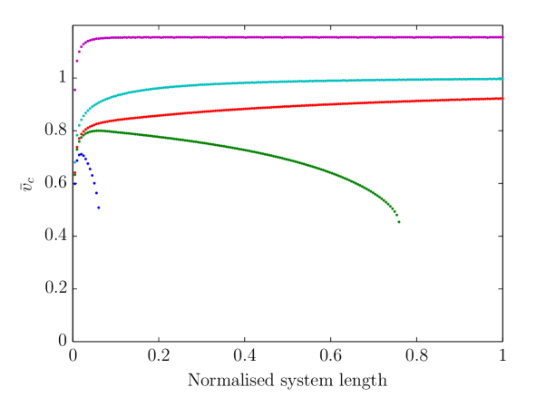
(a) Simulated front velocity as a function of position along the interface for several different values of $\bar{\tau}=\bar{f}^{+}$ obtained with $N=200$. From bottom to top, $\bar{\tau}=-0.1,\,-0.01,\,0.01,\,0.1,\,0.5$. Velocities are seen to approach a steady-state velocity for $\bar{\tau}>0$, while for $\bar{\tau}<0$ the fronts slow down and eventually arrest.

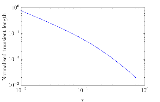
(b) Transient length, defined as the block number where the front velocity reaches $97\text{\,}\mathrm{\char 37\relax}\text{/}$ of the steady-state value, normalised by system size as a function of $\bar{\tau}$ obtained with $N=1000$.

Figure 2: Colour online. Rupture velocity as a function of position along the interface (a) and front velocity transient lengths (b) for various initial shear stress.

The straightforward way to compute the steady-state rupture velocity as a function of $\bar{\tau}$ is to solve Eqs. 23, 27, 31, 32, 33 and 39 explicitly in time for a given value of $\bar{\tau}$. Fronts go through a transient, as seen in Fig. 2a, before reaching the steady-state velocity. As shown in Fig. 2b, the transient length is strongly dependent on the pre-stress, $\bar{\tau}$, and extrapolation is necessary to estimate the final steady-state rupture velocity. We extrapolate the rupture velocity by fitting a first order polynomial to the curve $\bar{v}_{c}(1/n)$ for the last few ($\sim 50$) blocks towards the leading edge. These extrapolated steady-state velocities are plotted as a function of $\bar{\tau}$ in Fig. 3 as red circles.

Alternatively, equations for the steady-state front velocity can be derived from Eqs. 23, 27, 31, 32, 33 and 39. We provide this derivation in Section A.1, with Eqs. 74, 79, 76 and 77 the final set of equations. The numerical scheme used to solve these equations is detailed in Section B.2. We show in Fig. 3 the steady-state front velocity $\bar{v}_{c}$ as a function of $\bar{\tau}$ obtained by solving these equations numerically as blue crosses. This solution is seen to match the extrapolated front velocities obtained previously.

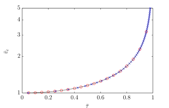
Figure 3: Colour online. Steady-state front velocity $\bar{v}_{c}$ as a function of initial stress, $\bar{\tau}$. $\bar{v}_{c}$ approaches $1$ as $\bar{\tau}\to 0$ and infinity as $\bar{\tau}\to 1$. Red circles are the extrapolated steady-state front velocities from simulations (as in Fig. 2a), blue crosses are the numerical solution of the steady-state equations (Section A.1), and the solid black line is the analytical solution given by Eq. 48.

It is also possible to solve the equations for the steady-state rupture velocity, Eqs. 74, 79, 76 and 77, analytically using an iterative approach. The solution technique is identical to the one used by Muratov (1999), and we present the detailed calculation in Section B.1. The result is a series expansion of $\bar{\tau}$ as a function of $z=1/\bar{v}_{c}$, given in Eq. 92. In the present case with $\bar{\eta}=0$, we get

$$\bar{\tau}=1-\frac{z^{2}}{2}-\frac{z^{4}}{8}-\frac{z^{6}}{16}-\frac{5z^{8}}{128}-\frac{7z^{10}}{256}+\mathcal{O}\left(z^{12}\right),$$ (46)

which we recognise as the series expansion of

$$\sqrt{1-z^{2}}=1-\frac{z^{2}}{2}-\frac{z^{4}}{8}-\frac{z^{6}}{16}-\frac{5z^{8}}{128}-\frac{7z^{10}}{256}+\mathcal{O}\left(z^{12}\right).$$ (47)

Consequently, we have a closed-form expression for the front velocity as a function of the initial shear stress:

$$\bar{\tau}=\sqrt{1-\bar{v}_{c}^{-2}}\quad\text{or}\quad\bar{v}_{c}=\frac{1}{\sqrt{1-\bar{\tau}^{2}}}.$$ (48)

This solution is plotted as the black solid line in Fig. 3, which matches the numerical results perfectly.

To summarise, the steady-state front velocity $\bar{v}_{c}$ in the model with AC friction and $\bar{\eta}=0$ only depends on the dimensionless initial shear stress, $\bar{\tau}$, and is given by Eq. 48, plotted in Fig. 3. The front velocity increases with increasing $\bar{\tau}$, as expected. All steady-state front velocities are supersonic, with values approaching the sound velocity as $\bar{\tau}\to 0$ and infinity as $\bar{\tau}\to 1$. The latter is easily explained: as $\bar{\tau}\to 1$, every block will be infinitely close to the static friction threshold, and infinitesimally small movement of the neighbouring blocks is enough to set them into motion. The time between the triggering of neighbouring blocks will therefore approach $0$, causing the front velocity to approach infinity, see Eq. 40. This is a known feature of spring-block models Knopoff (1997). We discuss these results in more detail in Section IV.

This model and the above results serve as our reference for investigating now the effect of a bulk viscosity and a tangential stiffness of the interface on the steady-state front velocity.

III.1.2 The effect of a bulk viscosity

In this section we study the effect of the relative viscosity $\bar{\eta}$, identical to the one used in Amundsen et al. (2012) to smooth grid-scale oscillations during front propagation Myers and Langer (1993); Shaw (1994). Physically it is a simple way of introducing energy dissipation that will occur during deformation. As in Section III.1.1 we have found that steady-state ruptures may occur if

$$0\leq\bar{\tau}<1,$$ (49)

independent of the value of the viscosity, $\bar{\eta}$. Similarly we have also found that blocks exclusively move in the positive direction as the front propagates along the interface. Consequently, we have two parameters controlling front velocity in this system, $\bar{\tau}$ and $\bar{\eta}$.

The steady-state equations are solved numerically as in Section III.1.1 for several different values of $\bar{\eta}$, and we plot $\bar{v}_{c}(\bar{\tau})$ in Fig. 4. As in the model with $\bar{\eta}=0$, the steady-state equations can be solved analytically, and the result is a series expansion of $\bar{\tau}$ in terms of $z=1/\bar{v}_{c}$ and $\bar{\eta}$. For brevity we do not reproduce this expansion here, it is given in Eq. 92.

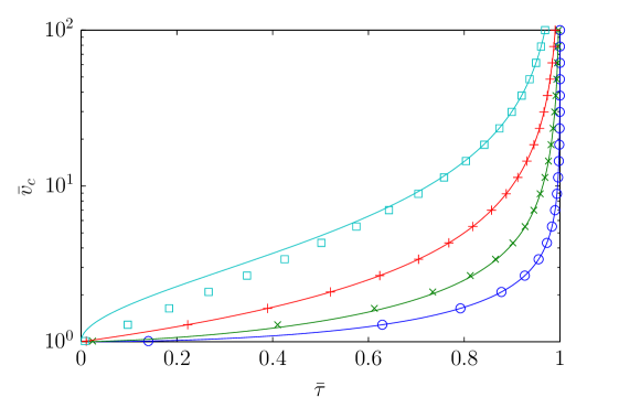
Figure 4: Colour online. Steady-state front velocity $\bar{v}_{c}$ as a function of initial shear stress, $\bar{\tau}$, for several different values of the relative viscosity $\bar{\eta}$. From bottom to top, $\bar{\eta}=0$ (blue, circles), $\sqrt{0.1}$ (green, crosses), $1$ (red, pluses) and $\sqrt{10}$ (cyan, squares). The point markers are the numerical solutions of the steady-state equations, and the solid lines are the semi-empirical closed-form expression in Eq. 54.

Unfortunately we have been unable to find a closed-form expression for the front velocity as a function of $\bar{\tau}$ and $\bar{\eta}$ from Eq. 92. The special case $\bar{\eta}=1$, however, yields

$$\bar{\tau}=1-z+\mathcal{O}\left(z^{12}\right),$$ (50)

i.e.

$$\bar{\tau}=1-\frac{1}{\bar{v}_{c}}\quad\text{or}\quad\bar{v}_{c}=\frac{1}{1-\bar{\tau}}.$$ (51)

We use this to derive a semi-empirical expression for $\bar{\tau}(\bar{v}_{c})$. From Eqs. 48 and 51, we can write

$$\bar{\tau}(\bar{v}_{c},\bar{\eta}=1)=\bar{\tau}(\bar{v}_{c},\bar{\eta}=0)\left(\frac{1-\bar{v}_{c}^{-1}}{1+\bar{v}_{c}^{-1}}\right)^{1/2}.$$ (52)

The factor $\left[(1-z)/(1+z)\right]^{1/2}$ can be thought of as a more general scaling factor including the $\bar{\eta}$ dependence, but taken at $\bar{\eta}=1$. We have found that we can estimate the $\bar{\eta}$ dependence with an exponent of $\bar{\eta}/2$, which fits the numerical solution fairly well. We therefore propose the following approximation

$$\bar{\tau}(\bar{v}_{c},\bar{\eta}) \approx\bar{\tau}(\bar{v}_{c},\bar{\eta}=0)\left(\frac{1-\bar{v}_{c}^{-1}}{1+\bar{v}_{c}^{-1}}\right)^{\bar{\eta}/2}$$ (53)

$$=\sqrt{1-\bar{v}_{c}^{-2}}\left(\frac{1-\bar{v}_{c}^{-1}}{1+\bar{v}_{c}^{-1}}\right)^{\bar{\eta}/2}.$$ (54)

We plot Eq. 54 in Fig. 4, and it is seen to match the numerical solution perfectly for $\bar{\eta}=0$ and $\bar{\eta}=1$ as expected, and to yield acceptable accuracy for $0\leq\bar{\eta}\leq 1$. The value of $\bar{\eta}=\sqrt{0.1}$ adopted by Amundsen et al. (2012) is within this range. The accuracy of the semi-empirical expression deteriorates for $\bar{\eta}>1$, which corresponds to a regime where all waves are overdamped Amundsen et al. (2012).

In Fig. 4 the relative viscosity is seen to not alter the limiting behaviour as $\bar{\tau}\to 0$ and $\bar{\tau}\to 1$, for which the front velocity still approaches $\bar{v}_{c}=1$ and $\bar{v}_{c}\to\infty$, respectively. An overall increase of front velocities compared to the $\bar{\eta}=0$ case, discussed in Section III.1.1, is, however, seen.

The reason for this particular behaviour is that the relative viscosity serves to dampen out (reduce) relative motion between blocks. At the front tip, the rightmost moving block is increasing the load on the leftmost stuck block through the material spring connecting them and through the relative viscous force. This viscous force acts in the direction of movement of the moving block. This causes the static friction threshold to be reached sooner, and the stuck block starts moving earlier than it would have with a smaller value of $\bar{\eta}$. Note that the stuck block will act with an equal and opposite force on the moving block, slowing it down. This effect remains small, however, due to the large momentum of the blocks behind the front tip. Overall, $\Delta\bar{t}_{n}$, the time between the rupture of block $n$ and $n+1$, is reduced.

III.2 Elasto-plastic like friction law

As discussed in Amundsen et al. (2012), in the model with AC friction, only the first block will experience the tangential loading force. This causes an unphysical resolution dependence in the model, which was improved considerably by introducing a finite tangential stiffness of the interface. In addition, the interface between the slider and the base is indeed elastic (see e.g. Prevost et al. (2013)), a feature which is often accounted for in models using an ensemble of interface springs to model the micro-contacts binding the slider and base together Braun and Peyrard (2008); Braun et al. (2009); Trømborg et al. (2014); Thøgersen et al. (2014); Trømborg et al. (2015).

We introduce a tangential stiffness of the interface as in Amundsen et al. (2012) by modifying the static Amontons–Coulomb friction law to include springs between the blocks and the track. Each block bears one interface spring having a breaking strength equal to the static friction threshold $\mu_{\text{s}}p$. When a spring breaks, dynamic friction $\mu_{\text{k}}p$ applies until the spring reattaches when the block velocity becomes zero. The spring is reattached such that at the time of reattachment the total force on the block is zero.

In this section we study front velocity as a function of $\bar{\tau}$ and the stiffness of the interface springs, $k_{\text{t}}$. For attached blocks the friction force is given by

$$f_{n} =-k_{\text{t}}\left(u_{n}(t)-u_{n}^{\text{stick}}(t)\right)$$

$$=-k_{\text{t}}\left(u_{n}^{\prime}(t)-{u_{n}^{\text{stick}}}^{\prime}(t)\right)-k_{\text{t}}\left(u_{n}(0)-u_{n}^{\text{stick}}(0)\right),$$ (55)

where $u_{n}^{\text{stick}}(t)$ is the position of the attachment point of the spring. At $t=0$ the total force on all blocks is zero, i.e. $f_{n}(t=0)=\tau_{n}$, and we get

$$f_{n}=-k_{\text{t}}\left(u_{n}^{\prime}(t)-{u_{n}^{\text{stick}}}^{\prime}(t)\right)-\tau_{n}.$$ (56)

Using Eq. 32 we obtain an expression for the dimensionless friction force,

$$\bar{f}_{n} =\frac{\tau_{n}-k_{\text{t}}\left(u_{n}^{\prime}(t)-{u_{n}^{\text{stick}}}^{\prime}(t)\right)-\tau_{n}}{\mu_{\text{s}}p_{n}-\mu_{\text{k}}p_{n}}$$ (57)

$$=-\frac{-k_{\text{t}}\left(u_{n}^{\prime}(t)-{u_{n}^{\text{stick}}}^{\prime}(t)\right)}{\mu_{\text{s}}p_{n}-\mu_{\text{k}}p_{n}}$$ (58)

$$=-\bar{k}\left(\bar{u}_{n}(t)-\bar{u}_{n}^{\text{stick}}(t)\right),$$ (59)

where $\bar{k}\equiv k_{\text{t}}/k$.

The rupture criterion is modified as it is a condition on the strength of the interface springs. It is given by

$$k_{\text{t}}\left(u_{n}(t)-u_{n}^{\text{stick}}(t)\right)=\mu_{\text{s}}p,$$ (60)

which in dimensionless variables becomes

$$\bar{k}\left(\bar{u}_{n}(t)-\bar{u}_{n}^{\text{stick}}(t)\right)+\bar{\tau}_{n}=1.$$ (61)

As discussed above, interface springs reconnect when the block velocity becomes zero and reconnect at zero total force:

$$0 =\bar{F}_{n}+\bar{F}_{n}^{\bar{\eta}}+\bar{f}_{n}$$ (62)

$$=\bar{F}_{n}+\bar{F}_{n}^{\bar{\eta}}-\bar{k}\left(\bar{u}_{n}(t)-{\bar{u}}_{n}^{\text{stick}}(t)\right),$$ (63)

which yields

$$\bar{u}_{n}^{\text{stick}}(t^{\text{stick}})=\bar{u}_{n}(t^{\text{stick}})-\frac{\bar{F}_{n}(t^{\text{stick}})+\bar{F}_{n}^{\bar{\eta}}(t^{\text{stick}})}{\bar{k}},$$ (64)

where the only new parameter introduced is the dimensionless interface stiffness $\bar{k}=k_{\text{t}}/k$, and $t^{\text{stick}}$ is the time at which the block velocity becomes zero. $\bar{u}_{n}^{\text{stick}}(t)$ stays constant for $t>t^{\text{stick}}$ until the block reattaches after another detachment event.

For simplicity we investigate the behaviour of this model without the relative viscosity here, $\bar{\eta}=0$, but this assumption is relaxed in Section III.3. As in Section III.1.1 we have investigated when steady-state ruptures occur and found that it is again restricted to

$$0\leq\bar{\tau}<1,$$ (65)

independent of the value of the interface stiffness, $\bar{k}$. Similarly we have also found that blocks exclusively move in the positive direction as the front propagates along the interface. Consequently, we have two parameters controlling the rupture velocity in this system, $\bar{\tau}$ and $\bar{k}$.

We solve the steady-state equations (derived in Section A.2) and show in Fig. 5 the front velocity as a function of the dimensionless initial shear force $\bar{\tau}$ for various values of the interface stiffness $\bar{k}$. In the limit $\bar{k}\to\infty$ the interface is infinitely stiff and the static friction law approaches AC’s friction law. As $\bar{k}$ decreases the front velocity also decreases and $\bar{v}_{c}\to 1$ in the $\bar{k}\to 0$ limit where the interface is infinitely soft.

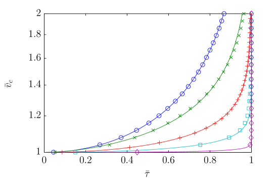
Figure 5: Colour online. Steady-state front velocity $\bar{v}_{c}$ as a function of initial shear stress, $\bar{\tau}$, for several different values of the interface stiffness $\bar{k}$. From top to bottom, $\bar{k}=${10}^{3}$,\,${10}^{1}$,\,$1$,\,${10}^{-1}$,\,${10}^{-3}$$. The crosses are the numerical solution, and the solid lines are the empirical closed-form expression in Eq. 66.

The rupture criterion, Eq. 61, is essentially a criterion for the displacement of a block relative to its attachment point. For a given pre-stress $\bar{\tau}$, as the interface stiffness $\bar{k}$ is reduced, blocks move a larger distance before detaching. In the limit $\bar{k}\to 0$ the rupture front will essentially become a displacement wave which moves with a velocity equal to the velocity of sound. This explains the behaviour of the model seen in the $\bar{k}\to 0$ limit.

Unfortunately we have not been able to obtain an analytical solution for the front velocity in the model with a tangential stiffness of the interface. Instead we have found the empirical expression

$$\bar{\tau}(\bar{v}_{c},\bar{k})=(1-\bar{v}_{c}^{-n_{1}})^{1/n_{2}},$$ (66)

where the coefficients $n_{1}$ and $n_{2}$ are functions of $\bar{k}$, to yield satisfactory agreement with the numerical solutions. Best fit values of the coefficients $n_{1}$ and $n_{2}$, for the values of $\bar{k}$ in Fig. 5, are given in Table 1. These were obtained by solving the steady-state equations (Section A.2) numerically as described in Section B.2 and fitting with Eq. 66 using a least squares method. The predictions made by Eq. 66 are shown as solid lines in Fig. 5.

$\bar{k}$	$n_{1}$	$n_{2}$
$10^{3}$	$2$	$2$
$10^{1}$	$3.75$	$1.7$
$10^{0}$	$7.86$	$1.97$
$10^{-1}$	$20.8$	$2.01$
$10^{-3}$	$106$	$2.87$

Table 1: Best fit coefficients to be used in the empirical expression for the front velocity given in Eq. 66. Note that the empirical approximation for $\bar{k}=${10}^{3}$$ is identical to Eq. 48.

III.3 Behaviour of the complete model

Figure 6 shows the evolution of front velocity as a function of pre-stress in the complete model, i.e. where both a relative viscosity and a tangential stiffness of the interface are included. Several values of $\bar{\eta}$ and $\bar{k}$ are used, demonstrating that the complete model behaves in a way qualitatively consistent with the results of Section III.1.2 and Section III.2. In particular, front speed increases both with increasing $\bar{\eta}$ and with increasing $\bar{k}$.

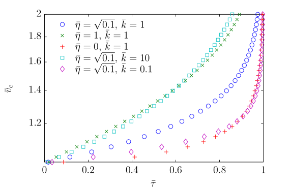
Figure 6: Colour online. Steady-state front velocity $\bar{v}_{c}$ as a function of initial shear stress, $\bar{\tau}$, for several different values of relative viscosity $\bar{\eta}$ and interface stiffness $\bar{k}$.

IV Discussion

We have found that, in general, the rupture front velocity increases with increasing pre-stress in our 1D spring-block-like models of extended frictional interfaces, as seen in Figs. 3, 4, 5 and 6. This is in agreement with observations on poly(methyl methacrylate) interfaces by Ben-David et al. (2010). We have also found the governing pre-stress parameter to be

$$\bar{\tau}\equiv\frac{\tau/p-\mu_{\text{k}}}{\mu_{\text{s}}-\mu_{\text{k}}}.$$ (67)

That is, in addition to the pre-stress $\tau$ itself, the steady-state rupture velocity also depends on the local friction parameters $\mu_{\text{s}}$ and $\mu_{\text{k}}$, and on the applied normal load through $p$. The same parameter $\bar{\tau}$ has successfully been applied to 2D spring-block models to scale non-steady-state front velocities obtained with different model parameters (see Fig. 4b in Trømborg et al. (2011), or Trømborg et al. (2015)). It is also equivalent to the $S$ ratio used in the geophysical literature Scholz (2002), defined as

$$S=\frac{\sigma_{\text{y}}-\sigma_{1}}{\sigma_{1}-\sigma_{\text{f}}},$$ (68)

where $\sigma_{\text{y}}$, $\sigma_{1}$ and $\sigma_{\text{f}}$ are the yield stress, initial stress and sliding frictional stress, respectively. In terms of the parameters in the model discussed here, $\sigma_{\text{y}}=\mu_{\text{s}}p$, $\sigma_{1}=\tau$, $\sigma_{\text{f}}=\mu_{\text{k}}p$, and we can express $S$ in terms of $\bar{\tau}$:

$$S=\frac{\mu_{\text{s}}-\tau/p}{\tau/p-\mu_{\text{k}}}=\frac{1}{\bar{\tau}}-1.$$ (69)

The parameter $\bar{\tau}$ is therefore much more general than the derivation from the present model alone would indicate.

The second parameter of importance to steady-state ruptures is the relative viscosity parameter $\bar{\eta}$ discussed in Section III.1.2. It provides a simple way of introducing energy dissipation that will occur during deformation of the slider and also removes resolution-dependent oscillations in Burridge–Knopoff-like models (Amundsen et al., 2012; Knopoff and Ni, 2001), with the recommended value $\bar{\eta}=\sqrt{0.1}$. Note that the viscosity $\eta$ considered here is a bulk viscosity affecting the relative motion of blocks. It is thus qualitatively different from an interfacial viscosity that would affect the absolute motion of a single block on the track, as was sometimes introduced at the micro-junction level in multi-junction models (see e.g. Braun et al. (2009)) or directly at mesoscales as a velocity strengthening branch of the friction law at large slip velocities (see e.g. Bar-Sinai et al. (2015)). In our case, the friction force on a block in the sliding state is $\mu_{\text{k}}p$, independent of slip speed. At a given $\bar{\tau}$, increasing $\bar{\eta}$ increases the steady-state front velocity, see Fig. 4. As discussed in Section III.1.2 this is due to the added shear force arising from the damping of relative motion between blocks. The particular choice $\bar{\eta}=\sqrt{0.1}$ (used in Amundsen et al. (2012); Trømborg et al. (2011)) is in Fig. 4 seen to only modestly increase the front velocity compared to $\bar{\eta}=0$.

The third and last parameter studied here is $\bar{k}=k_{\text{t}}/k$, the interface to bulk stiffness ratio, discussed in Section III.2. In Fig. 5 the limit $\bar{k}\to\infty$ is seen to yield Amontons–Coulomb-like behaviour, while decreasing $\bar{k}$ yields decreasing front velocities. In fact, as $\bar{k}\to 0$ the front velocity approaches the speed of sound as discussed earlier due to the front becoming a sound wave. These results should be relevant to various similar 1D and 2D models in which blocks are elastically connected to the base by springs Braun et al. (2009); Trømborg et al. (2011); Amundsen et al. (2012); Capozza and Urbakh (2012); Trømborg et al. (2014, 2015).

Recent simulations, in a 2D spring-block model with a friction law at the block scale emerging as the collective behaviour of many micro-junctions in parallel, have identified two different slip regimes for individual blocks Trømborg et al. (2014). A fast (inertial) slip regime is followed by a slow slip regime, controlled by the healing dynamics of the interface after rupture. Fronts driven by fast slip are fast inertial fronts, whereas fronts propagating when a significant portion of the slipping blocks are in the slow regime are slow Trømborg et al. (2015). In this context, all fronts observed in the present 1D models are of the fast type.

Although as seen in Fig. 2a the transient front velocity is often sub-sonic, in our model, all steady-state fronts are supersonic, i.e. $\bar{v}_{c}>1$. The fronts can propagate at arbitrarily large speeds as long as the pre-stress $\bar{\tau}$ is large enough. This has been discussed previously by Knopoff (1997). The velocity of sound in a 1D model is the longitudinal wave speed, while shear and Rayleigh waves do not exist. Nevertheless, we think it useful to point out that super-shear fronts have recently been observed in model experiments Ben-David et al. (2010), and that in the geophysical community, such fronts have been both predicted theoretically Freund (1979); Day (1982) and confirmed experimentally Rosakis et al. (1999); Bouchon and Vallée (2003); Xia et al. (2004); Schubnel et al. (2011).

As seen in Fig. 2b, and previously found in Trømborg et al. (2015), the initial transient in front speed before steady state is reached can be very long when $\bar{\tau}$ is close to zero. Because the dimensionless equations of motion do not change with the model resolution, it is clear that in this model, the length of the transients is given by a fixed number of blocks rather than a physical length, so we have overcome the problem of getting close to the steady state by performing simulations with a large number of blocks. In the other limit of $\bar{\tau}\to 1$, the transient length vanishes. We provide a demonstration of this result in Appendix C.

To investigate the transient length’s dependence on $\bar{\tau}$ for small values of $\bar{\tau}$ we initialise the system with a constant pre-stress as in Fig. 3 and let the rupture propagate until its velocity has reached $97\text{\,}\mathrm{\char 37\relax}\text{/}$ of the steady-state value. We define the point at which this happens as the transient length and plot in Fig. 2b the transient length as a function of $\bar{\tau}$. For small values of $\bar{\tau}$ the transient length is very large.

The above considerations emphasise the fact that in spring-block models like the one studied here it is important to choose the resolution carefully: this choice will indeed select the physical length of transients in front dynamics. The size of each block should be equal to the screening length Caroli and Nozières (1998), which in a purely elastic model is given by $\lambda_{d}\approx d^{2}/a$, where $d$ is the distance between micro-contacts and $a$ is the size of micro-contacts. For micrometer-ranged roughnesses, we expect $a\sim$1\text{\,}\mathrm{\SIUnitSymbolMicro m}\text{/}$$ and $d\sim\text{$10\text{\,}\mathrm{\SIUnitSymbolMicro m}\text{/}100\text{\,}\mathrm{\SIUnitSymbolMicro m}\text{/}$}$, yielding $\lambda\sim\text{$0.1\text{\,}\mathrm{mm}\text{/}10\text{\,}\mathrm{mm}\text{/}$}$, i.e. in the millimeter range. The typical horizontal length scale for extended lab-scale interfaces is $L\sim$100\text{\,}\mathrm{mm}\text{/}$$, which yields $N\sim 100$, which is consistent with the number of blocks used here or in our previous studies Trømborg et al. (2011); Amundsen et al. (2012); Trømborg et al. (2014, 2015).

Let us now compare our results to those of previous studies of steady state rupture velocities. In the Amontons–Coulomb case, our solution $v_{c}(\bar{\tau})$ takes the exact same form as the one found in Muratov (1999) for the Burridge–Knopoff model with Amontons–Coulomb friction (compare Eq. 92 and Eq. (A14) in Muratov (1999)). As in Muratov (1999), we find a well-defined continuum limit where rupture velocities do not depend on the chosen resolution. Compared to the studies in Langer and Tang (1991); Myers and Langer (1993) of the Burridge–Knopoff model with velocity weakening friction, our results are qualitatively, although not quantitatively, similar. In particular, we also find that the rupture velocity increases with increasing shear prestress of the interface and with increasing values of the viscous coefficient. Note that Langer and Tang (1991); Myers and Langer (1993); Muratov (1999) did not discuss the effect of an interfacial stiffness on rupture speed.

Trømborg et al. (2014, 2015) showed that, in their 2D model, the rupture and slip velocities are proportional. In 1D it is possible to derive a similar, exact relationship between the average slip speed and rupture velocity in the case of Amontons–Coulomb friction and no viscosity. This derivation is provided in Appendix D, where it is found that the local rupture velocity $\bar{v}_{c,i}$ at block $i$ in a simulation is related to the local average slip velocity $\dot{\bar{u}}_{i,\text{avg}}$ by

$$\bar{v}_{c,i}=\frac{\dot{\bar{u}}_{i,\text{avg}}}{1-\bar{\tau}}.$$ (70)

This relationship is demonstrated in Fig. 8, where we have plotted the local rupture velocity as a function of the local average slip velocity for various values of $\bar{\tau}$ as measured in simulations similar to those seen in Fig. 2a. Rescaling the average slip velocity by $1/(1-\bar{\tau})$, a straight line of unit slope is obtained. For comparison with the rescaling formula found by Trømborg et al. (2014, 2015), it is instructive to write Eq. 70 using dimensional quantities. Equations 40, 36 and 22 yield

$$v_{c,i}=\frac{\dot{u}_{i,\text{avg}}ak}{\mu_{\text{s}}p-\tau}=\frac{\dot{u}_{i,\text{avg}}ES}{\mu_{\text{s}}p-\tau},$$ (71)

where we have used $a=L/(N-1)$ and $k=(N-1)ES/L$ as in Amundsen et al. (2012), where $L$ is the length of the slider, $E$ is Young’s modulus and $S$ is the cross-sectional area of the slider. This strongly resembles the rescaling formula in Trømborg et al. (2014, 2015) which has the same denominator, while the characteristic force in the numerator is different due to the different interfacial laws applied.

An important question is whether the results obtained in the present 1D model can be extended to 2D models. To answer this question, we perform a series of simulations using the 2D model described in Trømborg et al. (2014, 2015), with model parameters suitable for the study of steady state front propagation. In particular, the slider’s length is twenty times larger than in Trømborg et al. (2014), so that front propagation has a chance to converge towards a steady state (the length of transients ranges from less than 40 blocks for $\bar{\tau}=0.95$ to longer than the system length for $\bar{\tau}=0.2$). We first choose a reference set of parameters, in which parameters are the same as in Table S1 of (Trømborg et al., 2014), except $L=$2.8\text{\,}\mathrm{m}\text{/}$$, $N_{x}=1140$, $M=$1.5\text{\,}\mathrm{kg}\text{/}$$, $F_{N}=$3840\text{\,}\mathrm{N}\text{/}$$, $\bar{\tau}_{\mathrm{trigger}}=0.95$, and $\alpha=\eta/160$. The rest of the settings are as follows: The width of the initial junction force distribution is zero, so the interface springs effectively act as a single spring per block. We checked that the mean junction slipping time $\bar{t}_{R}$, while important for slow fronts, does not affect these fast front results. Steady-state front velocity is estimated as in Section III.1.1, by fitting a straight line to $\bar{v}_{c}(1/n)$ for the last ($\sim N_{x}/2$) blocks towards the leading edge (excluding the last $\sim 40$, which have $\bar{v}_{c}$ increasing due to an edge effect).

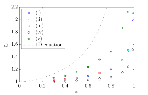
Figure 7: Colour online. Steady-state front velocity, $\bar{v}_{c}$, as a function of initial shear stress, $\bar{\tau}$, for simulations using the full 2D model of (Trømborg et al., 2014), for several different values of mass, damping coefficient, bulk stiffness and interface stiffness. Five sets of parameters were used: (i) Reference set; (ii) mass doubled and damping coefficient increased by a factor of $\sqrt{2}$, leaving $\bar{\eta}$ unchanged; (iii) bulk and interface stiffnesses halved, leaving $\bar{k}$ unchanged, (iv) damping coefficient and $\bar{\eta}$ reduced by a factor of $4$; and (v) interface stiffness and $\bar{k}$ increased by a factor of $10$. The dashed line plots Eq. 54 for the reference value of $\bar{\eta}$. Front speeds are normalized against the longitudinal bulk wave speed.

We first run simulations of the reference model for various values of $\bar{\tau}$ and plot the normalized steady state front speed $\bar{v}_{c}$ as a function of $\bar{\tau}$ in Fig. 7 (blue crosses). We observe that the results are qualitatively fully consistent with the behaviour in 1D, i.e. Fig. 6. In particular, the steady state front speed is always supersonic, tends towards the longitudinal bulk wave speed for small prestress and diverges for large prestress.

We then show that the two control parameters identified in 1D, $\bar{\eta}$ and $\bar{k}$, are also controlling the 2D front speed. To do this, we change model parameters (slider’s mass, damping coefficient, bulk and interfacial stiffnesses) in such a way that the rescaled parameters $\bar{\eta}$ and $\bar{k}$ are kept unchanged. Figure 7 clearly shows (see cyan dots and red squares) that these changes do not affect the values of $\bar{v}_{c}$.

Finally, we show that changes to the values of either $\bar{\eta}$ or $\bar{k}$ induce variations in the $\bar{v}_{c}(\bar{\tau})$ curve which are fully consistent with those observed in 1D (Fig. 6): decreasing $\bar{\eta}$ decreases the front speed (see black diamonds) whereas increasing $\bar{k}$ increases the front speed (green stars). All these results indicate that our main findings from the 1D model are not specific to 1D, but also hold in 2D, with the same non-dimensional control parameters and all the same qualitative characteristics.

V Conclusions

We have systematically studied the quantitative dependence of the steady-state rupture front velocity on pre-stress, damping and stiffness of the interface in a 1D spring-block model. We find that front velocity changes significantly by changing any of these parameters, the result of which can be seen in Figs. 3, 4, 5 and 6.

Increasing pre-stress leads to increasing rupture velocities, in agreement with both experiments Ben-David et al. (2010) and 2D models (see discussion and  Trømborg et al. (2011); Kammer et al. (2012); Trømborg et al. (2015)). Specifically, for the model with no viscosity and no finite stiffness of the interface, we derive a closed-form expression for the front velocity, given by Eq. 48. The dimensionless pre-stress parameter found to be controlling front velocities, $\bar{\tau}=(\tau/p-\mu_{\text{k}})/(\mu_{\text{s}}-\mu_{\text{k}})$, also depends on the strength of the interface through the frictional parameters $\mu_{\text{s}}$ and $\mu_{\text{k}}$. It is essentially a version of the $S$ ratio often used by the geophysical community Scholz (2002) and shown to also apply in 2D models Trømborg et al. (2011, 2015).

Material damping affects the front velocity through the parameter $\bar{\eta}=\eta/\sqrt{km}$. Increasing values of $\bar{\eta}$ are seen to yield increasing front velocities caused by the additional shear force. A semi-empirical expression for the dependence of the front velocity on $\bar{\eta}$ and $\bar{\tau}$ is given in Eq. 54.

Front velocities are seen to decrease with decreasing tangential stiffness of the interface through the parameter $\bar{k}=k_{\text{t}}/k$, i.e. the ratio between the shear stiffness of the interface and the material stiffness of the slider. An empirical expression for this dependence is given in Eq. 66. In fact, in the limit of a very soft interface compared to the material stiffness, steady-state rupture velocities are seen to approach the velocity of sound. The qualitative behaviour of all these parameters are seen to carry over to a model with both a finite stiffness of the interface and relative viscosity.

From Fig. 2b it is clear that transients can become very long, especially for low pre-stresses. This, coupled with a heterogeneous interface where $\bar{\tau}$ can be negative, suggests that experimentally observed rupture fronts like those in e.g. Rubinstein et al. (2004); Ben-David et al. (2010) may be dominated by transients. Direct comparison between these rupture fronts and the ones studied here may therefore not be possible, but the qualitative behaviour on parameters such as the internal damping and interface stiffness should remain valid.

Also note that viscoelastic materials have been shown in finite element simulations to exhibit memory effects. Stress concentrations left at the arrest location of one precursory slip event are not erased by the following rupture Radiguet et al. (2013). This causes non-homogeneous initial stresses for subsequent events. An interesting direction for future work would be to investigate the transient speeds resulting from such complicated stress states.

Despite the limitations of the model discussed above, it can provide valuable insight into rupture dynamics of frictional interfaces. We have shown here that the 1D results can be extended to a 2D model with the same interfacial law and bulk damping. Experimentally, it would be interesting to investigate the dependence of front velocities on the interface stiffness and bulk viscosity as they have been shown here to affect the rupture velocity significantly. Also, investigating the dependence of the front velocity on the system length would shed light on the influence of transients on observed ruptures.

Appendix A Deriving the equations for the steady-state rupture velocity

Here we derive the equations for steady-state rupture in the models discussed in this paper. We assume $\dot{u}_{n}(\bar{t})>0$ for all detached blocks, in agreement with the numerical solution of the equations for all cases where $\bar{f}^{+}>0$, as discussed in Section III. The system is considered to be infinitely long and the tangential driving velocity much smaller than the front velocity, we can therefore ignore the system boundaries.

A.1 Amontons–Coulomb friction

Here we derive the equations for the steady-state front velocity for the model with AC friction. As our starting point we use the dimensionless equations of motion, Eqs. 23, 27, 31, 39 and 43. Consequently, the controlling parameters in the equations of motion are $\bar{\tau}=\bar{f}^{+}$ and $\bar{\eta}$.

The equations of motion for moving blocks are given by

$$\ddot{\bar{u}}_{n} =\bar{u}_{n+1}-2\bar{u}_{n}+\bar{u}_{n-1}$$ (72)

$$\quad+\bar{\eta}(\dot{\bar{u}}_{n+1}-2\dot{\bar{u}}_{n}+\dot{\bar{u}}_{n-1})+\bar{\tau}.$$

To eliminate the dependence on $\bar{\tau}$ we introduce $\tilde{u}_{n}$ defined by

$$\bar{u}_{n}=\bar{\tau}\left(\tilde{u}_{n}+\bar{t}^{2}/2\right),$$ (73)

where the acceleration of blocks due to the force $\bar{\tau}$ is taken into account explicitly by the term $\bar{\tau}\bar{t}^{2}/2$ in Eq. 73. Equation 72 simplifies to

$$\ddot{\tilde{u}}_{n} =\tilde{u}_{n+1}-2\tilde{u}_{n}+\tilde{u}_{n-1}$$ (74)

$$\quad+\bar{\eta}(\dot{\tilde{u}}_{n+1}-2\dot{\tilde{u}}_{n}+\dot{\tilde{u}}_{n-1}),$$

which is our final equation of motion for moving blocks.

If the front is propagating at a constant velocity,

$$\bar{u}_{n}(\bar{t})=\bar{u}_{n+1}(\bar{t}+\Delta\bar{t}),\quad\dot{\bar{u}}_{n}(\bar{t})=\dot{\bar{u}}_{n+1}(\bar{t}+\Delta\bar{t}),$$ (75)

must hold, where $\Delta\bar{t}$ is the time between the triggering of two neighbouring blocks. It is therefore sufficient to consider the system in a time interval of length $\Delta\bar{t}$. We choose $\bar{t}\in\left[\bar{t}_{i},\bar{t}_{i}+\Delta\bar{t}\right]$, where block $i$ begins to move at $\bar{t}=\bar{t}_{i}$. For convenience, and without loss of generality, we choose $\bar{t}_{i}=0$. Using Eq. 73 this yields

$$\tilde{u}_{i}(0)=0,\quad\dot{\tilde{u}}_{i}(0)=0,$$ (76)

which is the initial condition for block $i$. For convenience we choose $i=0$.

The initial condition for Eq. 74 can be obtained by evaluating Eq. 75 at $\bar{t}=0$ and using Eq. 73. This yields

$$\tilde{u}_{n}(0) =\tilde{u}_{n+1}\left(\bar{v}_{c}^{-1}\right)+\frac{1}{2\bar{v}_{c}^{2}},$$ (77)

$$\dot{\tilde{u}}_{n}(0) =\dot{\tilde{u}}_{n+1}\left(\bar{v}_{c}^{-1}\right)+\frac{1}{\bar{v}_{c}},$$

since

$$\Delta\bar{t}=\frac{a/X}{\bar{v}_{c}}=\bar{v}_{c}^{-1}$$ (78)

from the definition of $X$, Eq. 22.

The equation of motion for all moving blocks is given by Eq. 74, but the equation of motion for block $i$ can be rewritten taking into account that block $i+1$ is stationary. Inserting $\bar{u}_{i+1}=0$ into Eq. 73 yields $\tilde{u}_{i+1}=-\bar{t}^{2}/2$, and using Eq. 74 with $n=i$ we have

$$\ddot{\tilde{u}}_{i} =\tilde{u}_{i-1}-2\tilde{u}_{i}-\bar{t}^{2}/2$$ (79)

$$\quad+\bar{\eta}(\dot{\tilde{u}}_{i-1}-2\dot{\tilde{u}}_{i}-\bar{t}),$$

Solving Eqs. 74, 79, 76 and 77 result in $\tilde{u}_{n}(\bar{t})$ for a given rupture velocity $\bar{v}_{c}$. This velocity is related to the parameter $\bar{\tau}$ through the rupture criterion, Eq. 42, at time $\bar{t}=0$ for block $i=0$. At $\bar{t}=0$ we have $\bar{u}_{0}(0)=\bar{u}_{1}(0)=\dot{\bar{u}}_{0}(0)=\dot{\bar{u}}_{1}(0)=0$, and using Eqs. 42, 27, 31 and 73 in addition to $\bar{\tau}=\bar{f}^{+}$ we get

$$\tilde{u}_{-1}(0)+\bar{\eta}\dot{\tilde{u}}_{-1}(0)=\frac{1-\bar{\tau}}{\bar{\tau}},$$ (80)

or equivalently

$$\bar{\tau}=\frac{1}{\tilde{u}_{-1}(0)+\bar{\eta}\dot{\tilde{u}}_{-1}(0)+1}$$ (81)

which relates the solution of Eqs. 74, 79, 76 and 77 for a given $\bar{v}_{c}$ to the corresponding $\bar{\tau}$. Note that these equations, in the case of $\bar{\eta}=0$, reduce to the equations determining the front velocity in the Burridge–Knopoff model using AC friction and the approximations of slow and soft tangential loading as derived by Muratov (1999).

A.2 Including a finite tangential stiffness of the interface

Here we derive the steady-state equations for the model including a tangential stiffness of the interface discussed in Section III.2. The equations of motion for sliding blocks are given by Eq. 74 as their equation of motion is identical to the AC case. For stuck blocks we combine Eqs. 23, 27, 31, 59 and 73 and get

$$\ddot{\tilde{u}}_{n} =\tilde{u}_{n+1}+\tilde{u}_{n-1}-2\tilde{u}_{n}$$ (82)

$$\quad+\bar{\eta}(\dot{\tilde{u}}_{n+1}-2\dot{\tilde{u}}_{n}+\dot{\tilde{u}}_{n-1})$$

$$\quad-\bar{k}(\tilde{u}_{n}+\bar{t}^{2}/2)-1,$$

where, without loss of generality, we have set $u_{n}^{\text{stick}}=0$. For convenience we again let block $i=0$ detach at $\bar{t}=0$, and by the same argument as above these equations need only to be solved for $\bar{t}\in[0,\Delta\bar{t}]$. The initial conditions are the same as for the AC case, Eq. 77, with the exception that only blocks far away from the rupture front keep a constant position. The initial conditions are therefore given by

$$\tilde{u}_{n-1}(0) =\tilde{u}_{n}(\bar{v}_{c}^{-1})+\frac{1}{2\bar{v}_{c}},$$ (83)

$$\dot{\tilde{u}}_{n-1}(0) =\dot{\tilde{u}}_{n}(\bar{v}_{c}^{-1})+\frac{1}{\bar{v}_{c}},$$

$$\tilde{u}_{n\to\infty} =\dot{\tilde{u}}_{n\to\infty}=0.$$

Using Eqs. 61 and 73 at $\bar{t}=0$ with $\bar{u}_{n}^{\text{stick}}=0$ we get

$$\bar{k}\tilde{u}_{n}(0)=\frac{1-\bar{\tau}}{\bar{\tau}},$$ (84)

which relates the solution of Eqs. 74, 82 and 83 for a given $\bar{v}_{\text{c}}$ to $\bar{\tau}$.

Appendix B Solving the equations for the steady-state rupture velocity

Here we solve for the steady-state velocity analytically using the equation set derived in Section A.1 for the model with AC friction. In addition we describe a numerical solution procedure that we use to solve the steady-state equations for the models with either AC or elasto-plastic friction laws.

B.1 Analytical solution of the Amontons–Coulomb steady-state rupture velocity equations

We solve Eqs. 74, 79, 76 and 77 using the iterative approach employed by Muratov (1999) where the solution is a power expansion in

$$z\equiv\bar{v}_{c}^{-1}.$$ (85)

If the front velocity is large, i.e. in the limit $z=\bar{v}_{c}^{-1}\to 0$, the distance required for block $0$ to move in order to initiate movement of block $1$ is negligible. Therefore, block $0$ is stationary in this limit. Also, when the rupture velocity is infinitely high, interactions between the blocks become less prominent because the time interval $\Delta\bar{t}$ becomes negligibly small.

To zeroth order in $z$, we therefore ignore the interaction terms in Eqs. 74 and 79, which yields $\ddot{\tilde{u}}_{n}^{(0)}=0$, i.e.

$$\tilde{u}_{n}^{(0)}=a_{n}^{(0)}\bar{t}+b_{n}^{(0)},$$ (86)

where $a_{n}^{(0)}$ and $b_{n}^{(0)}$ are constants to be determined from the initial condition. Using Eq. 77 we get the two coupled difference equations

$$a_{n}^{(0)} =a_{n+1}^{(0)}+z,$$ (87)

$$b_{n}^{(0)} =a_{n+1}^{(0)}z+b_{n+1}^{(0)}+\frac{1}{2}z^{2},$$ (88)

where $a_{0}^{(0)}=b_{0}^{(0)}=0$ from Eq. 76. The solution is

$$a_{n}^{(0)} =-nz,$$ (89)

$$b_{n}^{(0)} =\frac{n^{2}}{2}z^{2},$$ (90)

and we therefore have

$$\tilde{u}_{n}^{(0)}=-nz\bar{t}+\frac{n^{2}}{2}z^{2},\quad n\leq 0.$$ (91)

This is the first iteration, giving the zeroth order solution to Eqs. 74, 79, 76 and 77. The zeroth order relationship between $\bar{v}_{c}$ and $\bar{\tau}$ is obtained by using Eqs. 91 and 81.

The first order solution is obtained by substituting $\tilde{u}_{n}$ and $\dot{\tilde{u}}_{n}$ using Eq. 91 into Eqs. 74 and 79, integrating twice with respect to $\bar{t}$ and then using Eqs. 77 and 76 to eliminate the integration constants. This approach rapidly becomes cumbersome, so we have used Mathematica to go to higher orders. Here we simply give the solution:

$$\bar{\tau} =1\,-$$ (92)

$$\quad\,\,\frac{z}{1!}\bar{\eta}\,+$$

$$\quad\,\,\frac{z^{2}}{2!}(\bar{\eta}-1)(\bar{\eta}+1)\,+$$

$$\quad\,\,\frac{z^{3}}{3!}\bar{\eta}(\bar{\eta}-1)(\bar{\eta}+1)\,-$$

$$\quad\,\,\frac{z^{4}}{4!}(\bar{\eta}-1)(\bar{\eta}+1)(7\bar{\eta}^{2}-3)\,-$$

$$\quad\,\,\frac{z^{5}}{5!}\bar{\eta}(\bar{\eta}-1)(\bar{\eta}+1)(19\bar{\eta}^{2}-11)\,+$$

$$\quad\,\,\frac{z^{6}}{6!}(\bar{\eta}-1)(\bar{\eta}+1)(229\bar{\eta}^{4}-226\bar{\eta}^{2}+45)\,+$$

$$\quad\,\,\frac{z^{7}}{7!}\bar{\eta}(\bar{\eta}-1)(\bar{\eta}+1)(995\bar{\eta}^{4}-1154\bar{\eta}^{2}+295)\,-$$

$$\quad\,\,\frac{z^{8}}{8!}(\bar{\eta}-1)(\bar{\eta}+1)(17151\bar{\eta}^{6}-26837\bar{\eta}^{4}+12349\bar{\eta}^{2}-1575)\,-$$

$$\quad\,\,\frac{z^{9}}{9!}\bar{\eta}(\bar{\eta}-1)(\bar{\eta}+1)(102083\bar{\eta}^{6}-178177\bar{\eta}^{4}+95033\bar{\eta}^{2}-14971)\,+$$

$$\quad\,\,\frac{z^{10}}{10!}(\bar{\eta}-1)(\bar{\eta}+1)(2294141\bar{\eta}^{8}-4930384\bar{\eta}^{6}+3640514\bar{\eta}^{4}-1063816\bar{\eta}^{2}+99225)\,+$$

$$\quad\,\,O\left(z^{11}\right).$$

We conclude this section with a brief discussion of the validity of the solution in Eq. 92. It is valid only for $\bar{\tau}<1$ due to the form of the rupture criterion. It is not valid for $\bar{\tau}=0$ because of the transformation in Eq. 73. If $\bar{\tau}<0$, then $\bar{u}_{n}$ becomes negative (combine Eqs. 73 and 91). As a result, the velocity must be negative, but it was assumed to be positive. Equation 92 is consequently not valid for $\bar{\tau}\leq 0$, i.e., we get the constraints

$$0<\bar{\tau}<1,$$ (93)

which is consistent with the numerical results in Section III.

B.2 Numerical solution procedure

To solve the steady-state equations derived in Appendix A numerically, we used the following iterative scheme:

1. Select the desired $z=\bar{v}_{c}^{-1}$ for which the value of $\bar{\tau}$ is to be found. An initial guess for the position and velocity of all blocks must be made at $\bar{t}=0$, we used $\tilde{u}_{n}(0)=\dot{\tilde{u}}_{n}(0)=0$ as the initial guess for all results presented here.

2. Solve Equations 74 and 79 or Eqs. 74 and 82 using a numerical scheme for solving differential equations, e.g. the fourth order Runge–Kutta method.

3. Calculate a new estimate for the initial conditions using Eqs. 76 and 77 or Eq. 83 and the chosen front velocity. In the model with a tangential stiffness of the interface we have $\tilde{u}_{n\to\infty}=\dot{\tilde{u}}_{n\to\infty}=0$, which is implemented as $\tilde{u}_{N}=\dot{\tilde{u}}_{N}=0$ where $N$ is the number of blocks in the calculation. We find that $N=100$ yields satisfactory results. Calculate $\bar{\tau}$ using Eq. 81 or Eq. 84.

4. Repeat steps 2. and 3. until $\bar{\tau}$ has converged. The solution has converged when the difference in $\bar{\tau}$ between two iterations is less than some tolerance $\epsilon$. We use $\epsilon=${10}^{-6}$$.

The functions $\bar{v}_{c}(\bar{\tau})$ or equivalently $\bar{\tau}(\bar{v}_{c})$ can be calculated by repeating the above steps for several values of $\bar{v}_{c}$.

Appendix C Deriving the $\bar{\tau}\to 1$ limit of transient length

Here we show that in the limit of $\bar{\tau}\to 1$ the transient length vanishes by considering the motion of the trailing edge block as it begins to move.

Using Eqs. 23, 27, 31, 32 and 33 with AC friction [Eq. 44] the equation of motion for the trailing edge block becomes

$$\ddot{\bar{u}}_{\text{TE}}=-\bar{u}_{\text{TE}}+\bar{\tau}+\bar{F}_{\text{T}}$$ (94)

where we have set $\bar{\eta}=0$ for simplicity. As before we assume that $\bar{F}_{\text{T}}$ is independent of time. The initial condition for the trailing edge block is $\bar{u}_{\text{TE}}(\bar{t}=0)=\dot{\bar{u}}_{\text{TE}}(\bar{t}=0)=0$ and rupture initiates when $\bar{\tau}+\bar{F}_{\text{T}}=1$. This yields

$$\bar{u}_{\text{TE}}(\bar{t})=1-\cos\bar{t}.$$ (95)

The rupture criterion, Eq. 42, applied to the second block from the trailing edge yields

$$\bar{u}_{\text{TE}}(\bar{t}_{1})=1-\cos\bar{t}_{1}=1-\bar{\tau},$$ (96)

where $\bar{t}_{1}$ is the time at which the motion of the second block from the trailing edge is triggered. Noting that $z_{1}=\bar{t}_{1}=1/\bar{v}_{c,1}$, we have

$$\bar{\tau}=\cos z=1-\frac{z^{2}}{2}+\frac{z^{4}}{24}+\mathcal{O}(z^{6}).$$ (97)

Comparing with Eq. 46, the series of the steady-state rupture velocity, the first two terms are identical, i.e. as $\bar{\tau}\to 1$ ($z\to 0$), the rupture will instantly reach the steady-state velocity and the transient length approaches $0$. For smaller values of $\bar{\tau}$ (larger values of $z$), the transient length increases due to the deviations in the higher order terms.

Appendix D Slip speed vs rupture speed

Here we derive the relationship between the rupture and slip velocity in the model with Amontons–Coulomb friction and no viscosity. Consider block $i$, which started to move at time $\bar{t}=\bar{t}_{i}$, causing an increased shear force on block $i+1$. We only consider blocks moving in the positive direction, i.e. only $f_{i}^{+}=\bar{\tau}$ is required. The local rupture velocity is given by Eq. 78,

$$\bar{v}_{c,i}=\frac{1}{\Delta\bar{t}_{i}},$$ (98)

where $\bar{t}_{i}=\bar{t}_{i+1}-\bar{t}_{i}$ is the time between the triggering of block $i$ and $i+1$. The position of block $i$ at $\bar{t}_{i}$ is $\bar{u}_{i}=0$. The increase in shear force required for block $i+1$ to start moving is given by the rupture criterion, Eq. 42, and the position of block $i$ at $\bar{t}_{i+1}$ is therefore given by

$$\bar{u}_{i}(\bar{t}_{i+1})=1-\bar{\tau}.$$ (99)

The average slip velocity is consequently

$$\dot{\bar{u}}_{i,\text{avg}}=\frac{\bar{u}_{i}(\bar{t}_{i+1})-\bar{u}_{i}(\bar{t}_{i})}{\Delta\bar{t}_{i}}=\frac{1-\bar{\tau}}{\Delta\bar{t}_{i}},$$ (100)

and the rupture and slip velocities are related by

$$\bar{v}_{c,i}=\frac{\dot{\bar{u}}_{i,\text{avg}}}{1-\bar{\tau}}.$$ (70)

This relationship is demonstrated in Fig. 8, where we have plotted the local rupture velocity as a function of the local average slip velocity for various values of $\bar{\tau}$ as measured in simulations (similar to the simulations shown in Fig. 2a). Rescaling the average slip velocity by $1/(1-\bar{\tau})$, a straight line with unit slope is obtained.

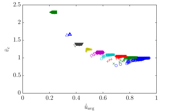
(a) Local rupture velocity $\bar{v}_{c}$ as a function of local slip velocity $\dot{\bar{u}}_{\text{avg}}$.

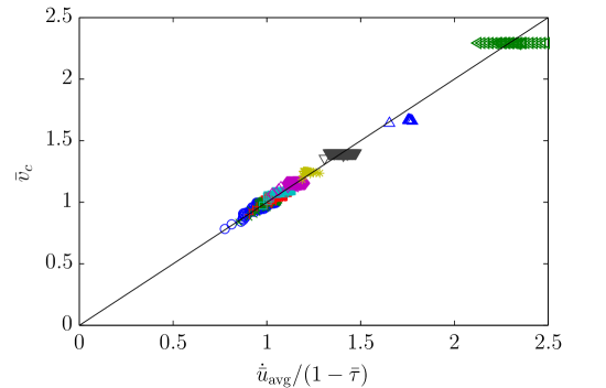
(b) Local rupture velocity $\bar{v}_{c}$ as a function of the rescaled local slip velocity $\dot{\bar{u}}_{\text{avg}}/(1-\bar{\tau})$. The black line is a straight line through the origin with a slope of unity as predicted by Eq. 70.

Figure 8: Colour online. Rupture velocity and slip velocity are closely related. These results have been obtained using simulations as in Fig. 2a for $\bar{\tau}=0.1,0.2,\dotsc,0.9$.

References

- Xia et al. (2004) K. Xia, A. J. Rosakis, and H. Kanamori, Science 303, 1859 (2004).
- Prevost et al. (2013) A. Prevost, J. Scheibert, and G. Debrégeas, Eur. Phys. J. E 36, 17 (2013).
- Romero et al. (2014) V. Romero, E. Wandersman, G. Debrégeas, and A. Prevost, Phys. Rev. Lett. 112, 094301 (2014).
- Rubinstein et al. (2004) S. M. Rubinstein, G. Cohen, and J. Fineberg, Nature 430, 1005 (2004).
- Ben-David et al. (2010) O. Ben-David, G. Cohen, and J. Fineberg, Science 330, 211 (2010).
- Schubnel et al. (2011) A. Schubnel, S. Nielsen, J. Taddeucci, S. Vinciguerra, and S. Rao, Earth Planet. Sci. Lett. 308, 424 (2011).
- Lu et al. (2007) X. Lu, N. Lapusta, and A. J. Rosakis, Proc. Natl. Acad. Sci. U. S. A. 104, 18931 (2007).
- Nielsen et al. (2010) S. Nielsen, J. Taddeucci, and S. Vinciguerra, Geophys. J. Int. 180, 697 (2010).
- Trømborg et al. (2011) J. Trømborg, J. Scheibert, D. S. Amundsen, K. Thøgersen, and A. Malthe-Sørenssen, Phys. Rev. Lett. 107, 074301 (2011).
- Kammer et al. (2012) D. S. Kammer, V. A. Yastrebov, P. Spijker, and J.-F. Molinari, Tribol. Lett. 48, 27 (2012).
- Trømborg et al. (2014) J. K. Trømborg, H. A. Sveinsson, J. Scheibert, K. Thøgersen, D. S. Amundsen, and A. Malthe-Sørenssen, Proc. Natl. Acad. Sci. U. S. A. 111, 8764 (2014).
- Amundsen et al. (2012) D. S. Amundsen, J. Scheibert, K. Thøgersen, J. Trømborg, and A. Malthe-Sørenssen, Tribol. Lett. 45, 357 (2012).
- Trømborg et al. (2015) J. K. Trømborg, H. A. Sveinsson, K. Thøgersen, J. Scheibert, and A. Malthe-Sørenssen, Phys. Rev. E 92, 012408 (2015).
- Ohnaka and Yamashita (1989) M. Ohnaka and T. Yamashita, J. Geophys. Res.: Solid Earth 94, 4089 (1989).
- Bar Sinai et al. (2012) Y. Bar Sinai, E. A. Brener, and E. Bouchbinder, Geophys. Res. Lett. 39, L03308 (2012).
- Rubinstein et al. (2007) S. M. Rubinstein, G. Cohen, and J. Fineberg, Phys. Rev. Lett. 98, 226103 (2007).
- Maegawa et al. (2010) S. Maegawa, A. Suzuki, and K. Nakano, Tribol. Lett. 38, 313 (2010).
- Scheibert and Dysthe (2010) J. Scheibert and D. K. Dysthe, Europhys. Lett. 96, 54001 (2010).
- Braun and Scheibert (2014) O. M. Braun and J. Scheibert, Tribol. Lett. 56, 553 (2014).
- Kammer et al. (2015) D. S. Kammer, M. Radiguet, J.-P. Ampuero, and J.-F. Molinari, Tribol. Lett. 57, 23 (2015).
- Braun et al. (2009) O. M. Braun, I. Barel, and M. Urbakh, Phys. Rev. Lett. 103, 194301 (2009).
- Capozza and Urbakh (2012) R. Capozza and M. Urbakh, Phys. Rev. B 86, 085430 (2012).
- Burridge and Knopoff (1967) R. Burridge and L. Knopoff, Bull. Seismol. Soc. Am. 57, 341 (1967).
- Carlson et al. (1994) J. M. Carlson, J. S. Langer, and B. E. Shaw, Rev. Mod. Phys. 66, 657 (1994).
- Kawamura et al. (2012) H. Kawamura, T. Hatano, N. Kato, S. Biswas, and B. K. Chakrabarti, Rev. Mod. Phys. 84, 839 (2012).
- de Sousa Vieira (1992) M. de Sousa Vieira, Phys. Rev. A 46, 6288 (1992).
- Milchev and Binder (1996) A. Milchev and K. Binder, Macromolecules 29, 343 (1996).
- Aumaître et al. (2001) S. Aumaître, S. Fauve, S. McNamara, and P. Poggi, Eur. Phys. J. B 19, 449 (2001).
- Blanc et al. (2014) B. Blanc, J.-C. Géminard, and L. Pugnaloni, Eur. Phys. J. E 37, 112 (2014).
- Langer and Tang (1991) J. S. Langer and C. Tang, Phys. Rev. Lett. 67, 1043 (1991).
- Myers and Langer (1993) C. R. Myers and J. S. Langer, Phys. Rev. E 47, 3048 (1993).
- Muratov (1999) C. B. Muratov, Phys. Rev. E 59, 3847 (1999).
- Kittel (2005) C. Kittel, Introduction to Solid State Physics, eighth ed. (John Wiley & Sons, Inc, Hoboken, 2005).
- Knopoff (1997) L. Knopoff, Annals of Geophysics 40, 1287 (1997).
- Shaw (1994) B. E. Shaw, Geophys. Res. Lett. 21, 1983 (1994).
- Braun and Peyrard (2008) O. M. Braun and M. Peyrard, Phys. Rev. Lett. 100, 125501 (2008).
- Thøgersen et al. (2014) K. Thøgersen, J. K. Trømborg, H. A. Sveinsson, A. Malthe-Sørenssen, and J. Scheibert, Phys. Rev. E 89, 052401 (2014).
- Scholz (2002) C. Scholz, The Mechanics of Earthquakes and Faulting (Cambridge University Press, 2002).
- Knopoff and Ni (2001) L. Knopoff and X. X. Ni, Geophys. J. Int. 147, 1 (2001).
- Bar-Sinai et al. (2015) Y. Bar-Sinai, R. Spatschek, E. A. Brener, and E. Bouchbinder, Sci. Rep. 5, 7841 (2015).
- Freund (1979) L. B. Freund, J. Geophys. Res.: Solid Earth 84, 2199 (1979).
- Day (1982) S. M. Day, Bull. Seismol. Soc. Am. 72, 1881 (1982).
- Rosakis et al. (1999) A. J. Rosakis, O. Samudrala, and D. Coker, Science 284, 1337 (1999).
- Bouchon and Vallée (2003) M. Bouchon and M. Vallée, Science 301, 824 (2003).
- Caroli and Nozières (1998) C. Caroli and P. Nozières, Eur. Phys. J. B 4, 233 (1998).
- Radiguet et al. (2013) M. Radiguet, D. S. Kammer, P. Gillet, and J.-F. Molinari, Phys. Rev. Lett. 111, 164302 (2013).