On Combining Estimation Problems Under Quadratic Loss: A Generalization

Abstract

The main theorem in Judge and Mittelhammer [Judge, G. G., and Mittelhammer, R. (2004), A Semiparametric Basis for Combining Estimation Problems under Quadratic Loss; JASA, 99, 466, 479–487] stipulates that, in the context of nonzero correlation, a sufficient condition for the Stein rule (SR)-type estimator to dominate the base estimator is that the dimension $k$ should be at least 5. Thanks to some refined inequalities, this dominance result is proved in its full generality; for a class of estimators which includes the SR estimator as a special case. Namely, we prove that, for any member of the derived class, $k\geqslant 3$ is a sufficient condition regardless of the correlation factor. We also relax the Gaussian condition of the distribution of the base estimator, as we consider the family of elliptically contoured variates. Finally, we waive the condition on the invertibility of the variance-covariance matrix of the base and the competing estimators. Our theoretical findings are corroborated by some simulation studies, and the proposed method is applied to the Cigarette dataset.

Keywords: Elliptically contoured variate; Least-squares estimators; Quadratic loss; Restricted estimator; Semiparametric inference; Shrinkage estimators; Stein-type estimator.

1 Introduction and statistical model

1.1 Introduction

The multiple regression model is a common statistical tool for investigating the relationship between a response variable and several explanatory variables. One of the main issues in regression analysis consists in estimating the regression coefficients. In particular, in the context of a linear regression model, it is common to use the ordinary least squares estimator (OLSE). Indeed, under the normality of the errors term, OLSE is known to be the maximum likelihood estimator as well as the minimum variance unbiased estimator. However, in case some prior information (from outside the sample) is available, OLSE may not be optimal. For instance, this prior information may be due to past statistical investigations, when these investigations could have concluded that some regression coefficients are not statistically significant. Another source of prior information may be the expertise in a certain field, which establishes an association between the regressor variables. Such a situation arises in economic theory where, for example, it is common to consider that the sum of the exponents in a Cobb-Douglas production (see Douglas and Cobb, 1928) is equal to one.

From the statistical inference point of view, it is important to incorporate the available prior information in the estimation method in order to improve upon the OLSE. For instance, if such prior information can be expressed in the form of exact linear restrictions binding the regression coefficients, instead of using the OLSE, one can resort to a competing estimator which is also known as the restricted least squares estimator (RLSE); it is known that the RLSE dominates the OLSE in such cases. In the sequel, the OLSE will be referred to as the base estimator while the RLSE will be referred to as the restricted estimator or the competing estimator. Thus, in the case where some exact prior information is available, the practitioners should use the restricted estimator in order to estimate the target parameter while if only the sample information is available, the base estimator is to be preferred.

Nevertheless, in some circumstances, the prior information is nearly correct and thus, we want to incorporate an additional information but we are not completely sure about it. Such uncertainty about the additional information may be induced by a change in the phenomenon underlying the regression model. Another context is the one where the prior information comes from experts in a field, the uncertainty reflects the imprecision in the experts’ information or judgements. In the case where the prior information is that, from the past statistical investigations, some regression coefficients are not statistically significant, the uncertainty may reflect the fact that a field specialist believes that the nonsignificant explanatory variables are important.

In these cases, we have to choose how to incorporate uncertain prior information into the inference procedure. Technically, in order to use both the sample and the uncertain prior, we can combine the base estimator and the restricted estimator and thus it is important to find an optimal combination. In the context of the linear regression model, Judge and Mittelhammer (2004) proposed a Stein-type estimator and derived a sufficient condition for the risk dominance of Stein-type estimator relative to a certain base estimator. However, the main result, in Judge and Mittelhammer (2004)[JM], has some limitations. First, the error term is supposed to be normally distributed. Second, the variance-covariance matrix of the joint distribution of the base estimator and the competing estimator is supposed to be invertible. This last assumption excludes, for example, a case where the prior information is about the non-significance of some regression coefficients. Third, the derived sufficient condition is too restrictive in the sense that it excludes the case of a multiple regression model with less than five regressors. Thus, the condition in JM (2004) is not applicable to the cases of quadratic or cubic regression models. However, in many applications (see Ashton et al., 2008, Fernandez-Juricic et al., 2003, among others), if a linear fit is not appropriate, a quadratic or cubic regression proves to be a simple and an adequate model. The last example is the Cigarette dataset produced by the USA Federal Trade Commission which can be found in Mendenhall and Sincich (1992). For this data set, the method in JM (2004) is not applicable since we have only three explanatory variables. In Section 4, we analyse this dataset and we show that our method performs very well.

In this paper, we generalize in four ways the main result in JM (2004) which gives a sufficient condition for the risk dominance of Stein-type estimator relative to a certain base estimator. First, we present a class of estimators which includes as a special case the Stein rule-type estimator given in JM (2004). Second, we relax the condition on the dimension of the parameter space. Third, we waive the condition on the invertibility of the variance-covariance matrix of the base estimator and the competing estimator. Thus, the proposed methodology works also in the case where the practitioners suspect some linear restrictions binding the regression coefficients. Fourth, we extend the main result to the case of a family of elliptically contoured distributions. To this end, recall that the normal distribution is a member of the elliptically contoured distributions, and, as explained in Provost and Cheong (2000), many test statistics and optimality properties underlying Gaussian random samples remain unchanged for elliptically contoured random samples. For further discussions and advantages of elliptically contoured distributions, we refer for example to Abdous et al. (2004), Liu et al. (2009) and references therein. Finally, the main key for establishing our results consists in deriving some inequalities and bounds which are more refined than that used in JM (2004).

The remaining of this paper is organized as follows. Section 1.2 presents the statistical model which is given in JM (2004) as well as the highlights of our contributions. In Section 2, we present a class of Stein rule-type of estimators and their risk function. Section 3 gives the main results of this paper in the Gaussian case and, more generally, in the elliptically contoured random case. We also show, in Section 3, that the proposed method works in the context where the variance-covariance of the base estimator and the competing estimator is singular. In Section 4, we present some simulation results for small sample sizes as well as an analysis of a real data set. Section 5 gives some concluding remarks. For the convenience of the reader, technical proofs are given in the Appendix.

1.2 Statistical model and main contributions

In this section, we recall the statistical model and the assumptions as well as some preliminary results which are given in JM (2004). Thus, this section presents only the model for which the error term is normally distributed. As mentioned in the Introduction, this is a preliminary step as we show later that the result established under the normality assumption holds also in the cases of elliptically contoured variables.

Following JM (2004), we consider the estimation problem of a $k$-dimensional location parameter vector when one observes an $n$-dimensional sample vector $y$ such that $y=\bm{X}\beta+\epsilon$, where $\bm{X}$ is an $n\times k$ design matrix of rank $k$ and $\epsilon$ is an $n$-dimensional random vector such that $\textrm{E}(\epsilon)=0$ and $\textrm{cov}(\epsilon)=\sigma^{2}\bm{I}_{n}$. Further, as in the quoted paper, we consider the scenario where there exists some uncertainty concerning the above statistical model, which leads to uncertainty concerning the appropriate inference method. For more details about these issues, we refer, for example, to JM (2004), Saleh (2006), Hossain et al. (2009), Morris and Lysy (2012) among others.

In the case where the above statistical model is appropriate, it is natural to estimate the target parameter $\beta$ by using the least-squares estimator (LS) $\hat{\delta}^{LS}=(\bm{X}^{\prime}\bm{X})^{-1}\bm{X}^{\prime}y$. Further, in the context of an alternative statistical model, one can consider the competing estimator $\tilde{\beta}$, which is such that $\textrm{E}(\tilde{\beta})=\beta+\gamma$, $\textrm{cov}(\tilde{\beta})=\bm{\Phi}$, $\textrm{cov}(\hat{\beta},\tilde{\beta})=\bm{\Sigma}$. Thus, as in JM (2004), the two estimators $\hat{\beta}$ and $\tilde{\beta}$ are assumed to be correlated, and $\tilde{\beta}$ may be biased with bias $\gamma$. In the context of uncertainty about which one of the two statistical models is more appropriate, it is common to consider an estimator which combines the two estimators in an optimal way. Originally, this type of method was introduced by James and Stein (1961). Over the last 50 years, numerous papers have been written around the topic so that it would be impossible to summarize all of them. To give some closely related references, we mention Bock (1975), Judge and Bock (1978), JM (2004), Saleh (2006), Nkurunziza and Ahmed (2010), Nkurunziza (2011), and Tan (2015) and references therein.

In our paper, we extend the following: JM (2004) stipulate that (see their main theorem), in the case of nonzero correlation between the base estimator $\hat{\beta}$ and the alternative estimator $\tilde{\beta}$, a sufficient condition for the Stein rule (SR)-type estimator to dominate the base estimator is $k\geqslant 5$.

In this paper, we extend this result in four ways. First, we construct a class of estimators which includes as a special case the SR estimator given in JM (2004). Second, we prove that, regardless of the presence of correlation, the condition $k\geqslant 3$ remains sufficient for any estimator of the proposed class of SR estimators to dominate in mean squared error the base estimator. The impact of this finding consists in the fact that, unlike the result in JM (2004), the established method can be applied to the case where the number of regressors is less than five as, for example, the case of a quadratic or a cubic regression model. Third, we also generalize the method in JM (2004) to the case where the joint distribution of the base estimator and the restricted estimator may be singular. This last result can be very useful in the case where the statistician suspects some linear restrictions binding the regression coefficients. This includes, for example, the case where the prior information from past statistical investigations is that some regression coefficients are not statistically significant, while the expert in the field of application believes that the corresponding explanatory variables should be in the model. Fourth, we prove that the established results hold if the normality assumption is replaced with that of elliptically contoured variates. Technically, in order to derive our findings, we establish some inequalities which are more refined than that in JM (2004). Finally, let us note that the simulation results are in agreement with the above theoretical findings. More specifically, the simulations show that the risk dominance of some SR estimators increases as the correlation increases.

2 A class of Stein rule estimators and the risk function

2.1 A class of Stein rule-type estimators

In this subsection, we present a class of Stein rule (SR)-type estimators which includes as a special case the SR estimator in JM (2004). First, recall that the results given in this paper hold under a very general statistical model than that in JM (2004). More precisely, the established results hold whenever the estimators $\hat{\beta}$ and $\tilde{\beta}$ follow jointly an elliptically contoured distribution. First, suppose that the estimators $\hat{\beta}$ and $\tilde{\beta}$ are jointly Gaussian. Thus, let

$$\left(\begin{array}[]{c}\hat{\beta}-\beta\\ \tilde{\beta}-\beta\\ \end{array}\right)\sim\mathcal{N}_{2k}\left((\bm{0},\bm{\gamma}^{\prime})^{\prime},\left(\begin{array}[]{cc}\bm{A}&\bm{\Sigma}\\ \bm{\Sigma}^{\prime}&\bm{\Phi}\\ \end{array}\right)\right),$$ (2.5)

where, as in JM (2004), the matrices $\bm{A}$, $\bm{\Phi}$, $\bm{\Xi}=\bm{A}-\bm{\Sigma}-\bm{\Sigma}^{\prime}+\bm{\Phi}$ are assumed to be positive definite. This assumption will be waived in Subsection 3.2 to study the case where the matrices $\bm{\Xi}$ and $\bm{\Phi}$ may be singular. Further, let $c$ be real number and let $h$ be real-valued measurable and square-integrable (with respect to the Gaussian measure). We consider the following class of SR estimators

$$\hat{\beta}^{S}(h,c)=\hat{\beta}+c\,\,h\left(\hat{\beta},\tilde{\beta}\right)\left(\hat{\beta}-\tilde{\beta}\right).$$ (2.6)

Example 2.1.

1. For a given $m$-column vector $e$,let $\|e\|^{2}=e^{\prime}e=\textrm{\em trace}(ee^{\prime})$. If $h\left(\hat{\beta},\tilde{\beta}\right)=1/\|\hat{\beta}-\tilde{\beta}\|^{2}$, for a known real number $c$, from (2.6), we get the estimator

   $$\hat{\delta}\left(\hat{\beta},\tilde{\beta};c\right)=\hat{\beta}-\displaystyle{\frac{c}{\|\hat{\beta}-\tilde{\beta}\|^{2}}}\left(\hat{\beta}-\tilde{\beta}\right),$$ (2.7)

   that is the Stein rule (SR)-type estimator given in JM (2004).

2. Let $\hat{a}=S^{2}\textrm{\em trace}((\bm{X}^{\prime}\bm{X})^{-1})-\textrm{\em trace}(\hat{\bm{\Sigma}})$, $S^{2}=(n-k)^{-1}\|y-\bm{X}\hat{\beta}\|^{2}$, $\hat{\bm{\Sigma}}$ is an unbiased and/or a consistent estimator for $\bm{\Sigma}$. If $c=-\hat{a}$, $h\left(\hat{\beta},\tilde{\beta}\right)=1/\|\hat{\beta}-\tilde{\beta}\|^{2}$, the estimator in (2.6) becomes the Semiparametric Stein-Like (SPSL) estimator given in JM (2004). Namely, we have

   $$\hat{\beta}^{S}=\hat{\beta}-\displaystyle{\frac{\hat{a}}{\|\hat{\beta}-\tilde{\beta}\|^{2}}}(\hat{\beta}-\tilde{\beta}).$$ (2.8)

3. If $h\left(\hat{\beta},\tilde{\beta}\right)=0$, the estimator in (2.6) yields the base estimator $\hat{\beta}$.

4. If $c=-1$, $h\left(\hat{\beta},\tilde{\beta}\right)=1$, we have $\hat{\beta}^{S}(-1,1)=\tilde{\beta}$.

As an important point, in this paper, the random quantity $h\left(\hat{\beta},\tilde{\beta}\right)$ is a statistic in the sense that it can be computed whenever we have the observations. As for the real value $c$ which is assumed to be known in (2.6), this is similar to that used in SR-estimator in JM (2004). The impact of replacing $c$ by its corresponding consistent estimator should be similar to that in JM (2004). In practice, the value of $c$ can be obtained by using a re-sampling technique as the bootstrap.

2.2 Risk function

The performance of the proposed class of estimators is studied under the quadratic loss function. Thus, the quadratic risk function, so-called the mean squared error (MSE), of the class of the estimators in (2.6) is

$$\textrm{MSE}\left(\hat{\beta}^{S}(h,c)\right)=\textrm{E}\left[\left(\hat{\beta}^{S}(h,c)-\beta\right)^{\prime}\left(\hat{\beta}^{S}(h,c)-\beta\right)\right].$$

then, by using (3.5) and (3.6), we have

$$\textrm{MSE}\left(\hat{\beta}^{S}(h,c)\right)=\textrm{trace}(\bm{A})-2c\eta(h)+c^{2}\omega(h),$$ (2.9)

where

$$\eta(h)=\textrm{E}\left[h\left(\hat{\beta},\tilde{\beta}\right)\left(\hat{\beta}-\beta\right)^{\prime}\left(\hat{\beta}-\tilde{\beta}\right)\right],\quad{}\omega(h)=\textrm{E}\left[h^{2}\left(\hat{\beta},\tilde{\beta}\right)\left\|\hat{\beta}-\tilde{\beta}\right\|^{2}\right],$$ (2.10)

assuming that these expectations are defined. Thus, from (2.9), it is obvious that, for all $c\in\left(\min\{0,2\eta(h)/\omega(h)\},\,\max\{0,2\eta(h)/\omega(h)\}\right)$, we have

$$\textrm{MSE}\left(\hat{\beta}^{S}(h,c)\right)<\textrm{MSE}(\hat{\beta}),$$

provided that $\eta(h)$ and $\omega(h)$ exist. Further, from (2.9), one concludes that the optimal choice of $c$ is $c_{*}=\eta(h)/\omega(h)$ and thus,

$$\textrm{MSE}\left(\hat{\beta}^{S}(h,c^{*})\right)=\textrm{trace}(\bm{A})-(\eta^{2}(h)/\omega(h)).$$ (2.11)

Remark 2.1.

Assuming that $\eta(h)$ and $\omega(h)$ are defined, (2.11) implies that, for a fixed value of $\omega(h)$, the MSE of the SR estimator decreases as $\eta(h)$ increases. Further, for a fixed value of $\eta(h)$, the MSE of the SR estimator decreases as $\omega(h)$ decreases. The simulation results given in Section 4.1 are in agreement with this analysis. To make this idea more precise, we first note that, for a given $h$, the values of $\omega(h)$ and $\eta(h)$ depend both on $\gamma$, the bias of the estimator $\tilde{\beta}$, and on the covariance between the estimator $\tilde{\beta}$ and $\hat{\beta}$. In particular, the simulation results show that the risk dominance of the SPSL increases as the correlation increases. Also, the simulation results show that the risk dominance of the SPSL decreases as the norm of the bias increases.

As mentioned above, the derivation of the MSE in (2.9) and (2.11) assumes the existence of $\omega(h)$ and $\eta(h)$. Thus, it is important to derive the conditions under which these expectations are defined. To this end, we require that the function $h$ satisfies the following assumption.

Assumption $(\mathcal{H}_{1})$: The function $h$ is such that $\|x-y\|^{2}|h(x,y)|$ is bounded i. e.

$$|h(x,y)|=O\left(\|x-y\|^{-2}\right).$$

Remark 2.2.

It should be noticed that the function $h$ which gives the SR estimator satisfies the above assumption. Indeed, in this case, we have $\|x-y\|^{2}|h(x,y)|=1$. Also, the function $h\equiv 0$ which gives the base estimator satisfies the above assumption. As another example of a function $h$ which satisfies the Assumption $(\mathcal{H}_{1})$, one can take $h(x,y)=\displaystyle{\frac{1}{1+\|x-y\|^{p}}}$ for some $p\geqslant 2$.

Below, we prove that, under the above assumption, regardless of the presence of correlation, the condition $k\geqslant 3$ remains sufficient for any estimator of the class in (2.6) to dominate in mean square error the base estimator. In particular, since the SR estimator is a member of the class of the estimators in (2.6), the established result proves that, regardless of the presence of correlation, the condition $k\geqslant 3$ remains sufficient for the SR estimator to dominate in mean square error the base estimator. We also prove that this conclusion holds if the normality assumption is replaced by that of elliptically contoured variates.

3 Main results

In this section, we present the main results of this paper. As an intermediate step, we derive below three propositions and a theorem which play a central role in deriving the main result. In summary, these results are useful in deriving a more refined inequality than that used in JM (2004). In order to simplify the presentation of the main results, we define some notations which will be used for the remaining of the paper. Let $U=(U^{\prime}_{1},U^{\prime}_{2})^{\prime}$ where $U_{1}=\hat{\beta}-\beta$ and $U_{2}=\tilde{\beta}-\beta$. From (2.5), we have

$$U=\left(\begin{array}[]{c}U_{1}\\ U_{2}\\ \end{array}\right)\sim\mathcal{N}_{2k}\left((\bm{0},\bm{\gamma}^{\prime})^{\prime},\left(\begin{array}[]{cc}\bm{A}&\bm{\Sigma}\\ \bm{\Sigma}^{\prime}&\bm{\Phi}\\ \end{array}\right)\right).$$ (3.5)

From the Cholesky decomposition, let $\bm{P}$ be a nonsingular matrix such that $\bm{\Xi}=\bm{P}\bm{P}^{\prime}$, and let

$$Z=\bm{P}^{-1}(U_{1}-U_{2})\quad{}\mbox{ and }\quad{}\bm{R}=\bm{P}^{\prime}\bm{P}.$$ (3.6)

Further, let

$$W=\left(\begin{array}[]{c}U_{1}\\ Z\\ \end{array}\right),\quad{}\bm{F}=\left(\begin{array}[]{cc}\bm{0}&\bm{0}\\ \bm{P}&\bm{0}\\ \end{array}\right),\quad{}\bm{B}=\left(\begin{array}[]{cc}\bm{0}&\bm{P}^{\prime}\\ \bm{P}&\bm{0}\\ \end{array}\right),$$ (3.13)

$$\eta=\textrm{E}\left[U^{\prime}_{1}\bm{P}Z\,/Z^{\prime}\bm{R}Z\right],\quad{}\eta^{{\ddagger}}=\textrm{E}\left[|U^{\prime}_{1}\bm{P}Z|\,/Z^{\prime}\bm{R}Z\right],\quad{}\omega=\textrm{E}\left[1\,/Z^{\prime}\bm{R}Z\right].$$ (3.14)

Proposition 3.1.

Suppose that Assumption $(\mathcal{H}_{1})$ holds, then there exists $q_{\scriptscriptstyle 0}>0$ such that

1. $|\eta(h)|\leqslant q_{\scriptscriptstyle 0}\eta^{{\ddagger}}$ where $\eta^{{\ddagger}}$ is defined in (3.14);

2. $|\omega(h)|\leqslant q^{2}_{\scriptscriptstyle 0}\omega$ where $\omega$ is defined in (3.14).

The proof of this proposition is given in the Appendix. From Proposition 3.1, it is clear that, in order to prove that $\eta(h)$ and $\omega(h)$ are defined, it is sufficient to prove that $\eta^{{\ddagger}}<\infty$ and $\omega<\infty$. Below, we establish a theorem which proves that, provided that $k\geqslant 3$, $\omega<\infty$, and this implies that $\eta^{{\ddagger}}<\infty$. To introduce some notations, let $\mathbb{I}_{G}$ denote the indicator function of the event $G$, let $H$ be $k\times k$-symmetric matrix, let $\lambda(\bm{H})$ denote the eigenvalue of $\bm{H}$, and let $\lambda_{1}(\bm{H})$, $\lambda_{2}(\bm{H})$, $\dots$, $\lambda_{k}(\bm{H})$ be respectively the first, the second, $\dots$, the $\mbox{k}^{th}$ the eigenvalue of $\bm{H}$.

Proposition 3.2.

Let $\alpha>0$, let $\psi_{1}=\max\{|\lambda_{1}(\bm{B})|,|\lambda_{2}(\bm{B})|,\dots,|\lambda_{2k}(\bm{B})|\}$, where $\bm{B}$ is defined in (3.13), and let $W$ be the random vector in (3.13). We have

$$\textrm{\em E}\left\{\left(|U_{1}^{\prime}\bm{P}Z|\,\big{/}Z^{\prime}\bm{R}Z\right)\,\mathbb{I}_{\left\{\|W\|\leqslant\alpha\right\}}\right\}\leqslant\alpha^{2}\,\psi_{1}\,\omega\,/2.$$ (3.15)

The proof of this proposition is given in the Appendix.

Proposition 3.3.

Let $\alpha>0$, and let $\psi_{0}=\min\{\lambda_{1}(\bm{R}),\lambda_{2}(\bm{R}),\dots,\lambda_{k}(\bm{R})\}$. We have

$$\textrm{\em E}\left\{\left(|W^{\prime}\bm{F}W|\,\big{/}\,Z^{\prime}\bm{R}Z\right)\mathbb{I}_{\left\{\|W\|>\alpha\right\}}\right\}\leqslant\psi_{1}\,\left[\textrm{\em trace}(\bm{A})+k+\mu^{\prime}\mu\right]\,\big{/}(\alpha^{2}\,\psi_{0}).$$ (3.16)

The proof of this proposition is given in the Appendix. By combining Propositions 3.2 and 3.3, we establish the following theorem which plays a central role in proving that $\eta$ exists whenever $0<\omega<+\infty$.

Theorem 3.4.

Let $\alpha>0$, then there exists $M(\alpha)>0$ such that

$$|\eta|\leqslant\eta^{{\ddagger}}<M(\alpha)\omega+\,\psi_{1}\,\left(\textrm{\em tr}\left(\bm{A}\right)+k+\mu^{\prime}\mu\right)\,\big{/}(\alpha^{2}\psi_{0}),$$ (3.17)

where $\psi_{1}$ and $\psi_{0}$ are given in Propositions 3.2 and 3.3 respectively.

Proof.

Since $\bm{R}$ is a positive definite matrix, we have

$$|\eta|\leqslant\textrm{E}\left[|U^{\prime}_{1}\bm{P}Z|\,\big{/}(Z^{\prime}\bm{R}Z)\right]=\textrm{E}\left[|\left(Z^{\prime},U^{\prime}_{1}\right)\bm{F}\left(Z^{\prime},U^{\prime}_{1}\right)^{\prime}|\,\big{/}(Z^{\prime}\bm{R}Z)\right],$$ (3.18)

where $\bm{F}$ is given in equation (3.13). Further, set $W=\left(Z^{\prime},U^{\prime}_{1}\right)^{\prime}$. We have,

$$\textrm{E}\left[\frac{|W^{\prime}\bm{F}W|}{Z^{\prime}\bm{R}Z}\right]=\textrm{E}\left\{\frac{|W^{\prime}\bm{F}W|}{Z^{\prime}\bm{R}Z}\mathbb{I}_{\left\{\|W\|>\alpha\right\}}\right\}+\textrm{E}\left\{\frac{|W^{\prime}\bm{F}W|}{Z^{\prime}\bm{R}Z}\mathbb{I}_{\left\{\|W\|\leqslant\alpha\right\}}\right\}.$$ (3.19)

Then, by combining Propositions 3.2 and 3.3 and by taking $M(\alpha)=\alpha^{2}\psi_{1}/2$, we get the stated result. ∎

By using Theorem 3.4, we establish the following corollary which shows that $\eta^{{\ddagger}}$ (and so $|\eta|$) is bounded by a positive real number which is finite provided that $0<\omega<+\infty$.

Corollary 3.5.

Suppose that the conditions of Theorem 3.4 hold. Then,

$$|\eta|\leqslant\eta^{{\ddagger}}<\omega+\,\psi_{1}^{2}\,\left(\textrm{\em trace }\left(\bm{A}\right)+k+\mu^{\prime}\mu\right)\,\big{/}(2\psi_{0}),$$

where $\psi_{1}$ and $\psi_{0}$ are given in Propositions 3.2 and 3.3 respectively.

Proof.

For $\alpha=\sqrt{2/\psi_{1}}$, we have $M(\alpha)=\alpha^{2}\psi_{1}/2=1$. Then, by using Theorem 3.4, we get the statement of the corollary. ∎

Remark 3.1.

It should be noticed that Propositions 3.2-3.3, Theorem 3.4, and Corollary 3.5 hold even in the case where $W$ is not Gaussian, provided that the mean and the variance-covariance matrix of $U$ are the same as the one given in (3.5).

Remark 3.2.

From Corollary 3.5, it should be noticed that, if $0<\omega<\infty$, then $|\eta|\leqslant\eta^{{\ddagger}}<\infty$. This is an interesting finding which shows that the nonzero correlation does not affect the condition for the risk dominance of the SR estimator relative to the base estimator. Thus, under normality, in order to guarantee the existence of the MSE in (2.9) and (2.11), it is sufficient to let $k\geqslant 3$.

Corollary 3.6.

Under normality, $k\geqslant 3$ implies $0<\omega<+\infty$ and $|\eta|\leqslant\eta^{{\ddagger}}<+\infty$.

Proof.

If $k\geqslant 3$, from the proof in JM (2004), $0<\omega<+\infty$. Then, by using Theorem 3.4, we get $|\eta|\leqslant\eta^{{\ddagger}}<+\infty$. ∎

Corollary 3.7.

Suppose that Assumption $(\mathcal{H}_{1})$ holds. Under normality, $k\geqslant 3$ implies $0<\omega(h)<+\infty$ and $|\eta(h)|<+\infty$.

The proof follows from Proposition 3.1 and Corollary 3.6.

Note that Corollary 3.6 generalizes the main theorem in JM (2004). Further, Corollary 3.7 extends the result of Corollary 3.6 to a class of SR-type estimators which includes the SR-type estimator in JM (2004) as a special case.

3.1 Extension to elliptically contoured random samples

In this subsection, we show that the result given in Corollary 3.6 remains valid in the context of some elliptically contoured random samples. The importance of such a family of distributions is the primary source of our motivation. Indeed, as discussed in the literature, elliptically contoured distributions have been particularly useful in several areas of applications such as actuarial science (see Furman and Landsman, 2006, Landsman and Valdez,  2003), or economics and finance (see Bingham and Kiesel, 2001).

Recall that a class of elliptically contoured distributions includes for example the multivariate Gaussian, t, Pearson type II and VII, as well as Kotz distributions. To simplify the notation, let $X\sim\mathcal{E}_{q}\left(\mu,\,\bm{\Sigma};g\right)$ stand for a $q$-column random vector distributed as an elliptically contoured vector with mean $\mu$ and scale parameter matrix $\bm{\Sigma}$, where $\bm{\Sigma}$ is a positive definite matrix, and $g$ is the probability density function (p.d.f) generator. For the sake of simplicity, we consider the case where the p.d.f of $X\sim\mathcal{E}_{q}\left(\mu,\,\bm{\Sigma};g\right)$ is assumed to be written as

$$f_{X}(x)=\displaystyle{\int_{0}^{\infty}}f_{\mathcal{N}\left(\mu,\,z^{-1}\bm{\Sigma}\right)}(x)\kappa(z)dz,$$ (3.20)

where $f_{\mathcal{N}\left(\mu,\,\bm{\Sigma}\right)}$ denotes the p.d.f of a random vector which follows a normal distribution with mean $\mu$ and variance-covariance $\bm{\Sigma}$, and $\kappa(.)$ is a weighting function that satisfies $\displaystyle{\int_{0}^{\infty}}\displaystyle{\frac{1}{t}}\left|\kappa(t)\right|\,dt<\infty$. Note that the weighting function $\kappa(.)$ does not need to be nonnegative. In the case where the function $\kappa(.)$ is nonnegative, then $\kappa(.)$ is a p.d.f, and the subclass of elliptically contoured distributions is known as a mixture of multivariate normal distributions. For more details, we refer to Chmielewski (1981), Gupta and Verga (1995), Nkurunziza and Chen (2013) among others. In particular, Gupta and Verga (1995) give the conditions on the p.d.f generator $g$ for the pdf of $X\sim\mathcal{E}_{q}\left(\mu,\,\bm{\Sigma};g\right)$ to be rewritten as in (3.20). From now on, we suppose that $\left((\hat{\beta}-\beta)^{\prime},\,(\tilde{\beta}-\beta)^{\prime}\right)^{\prime}$ has a p.d.f which can be rewritten as in  (3.20), and in a similar way to Section 2, let

$$U=\left(\begin{array}[]{c}U_{1}\\ U_{2}\\ \end{array}\right)=\left(\begin{array}[]{c}\hat{\beta}-\beta\\ \tilde{\beta}-\beta\\ \end{array}\right)\sim\mathcal{E}_{2k}\left((0,\gamma^{\prime})^{\prime},\left(\begin{array}[]{cc}\bm{A}&\bm{\Sigma}\\ \bm{\Sigma}^{\prime}&\bm{\Phi}\\ \end{array}\right);g\right),$$ (3.27)

where $\gamma$, $\bm{A}$, $\bm{\Sigma}$, $\bm{\Phi}$ are as defined in Section 2.

Theorem 3.8.

Suppose that $\left((\hat{\beta}-\beta)^{\prime},\,(\tilde{\beta}-\beta)^{\prime}\right)^{\prime}$ is distributed as in (3.27) and suppose that the weighting function $\kappa(.)$ satisfies   $0<\displaystyle{\int_{0}^{\infty}}t\left|\kappa(t)\right|\,dt<\infty$. Then, $k\geqslant 3$ implies $0<\omega<+\infty$ and $|\eta|\leqslant\eta^{{\ddagger}}<+\infty$.

Proof.

First, recall that the family of elliptically contoured distribution is closed under linear transformations. Then, if $\left((\hat{\beta}-\beta)^{\prime},\,(\tilde{\beta}-\beta)^{\prime}\right)^{\prime}$ is distributed as in (3.27), (2.9) and (2.11) hold, and then (3.14) holds with $Z\sim\mathcal{E}_{k}\left(\mu,\bm{I}_{k};g\right)$. Therefore, by using Remark 3.1, we conclude that Corollary (3.5) holds. Further, as in JM (2004), we get

$$\displaystyle{\frac{1}{\max\left(\lambda_{1}(\bm{R}),\lambda_{2}(\bm{R}),\dots,\lambda_{k}(\bm{R})\right)}}\textrm{E}\left(\frac{1}{Z^{\prime}Z}\right)<\omega<\displaystyle{\frac{1}{\min\left(\lambda_{1}(\bm{R}),\lambda_{2}(\bm{R}),\dots,\lambda_{k}(\bm{R})\right)}}\textrm{E}\left(\frac{1}{Z^{\prime}Z}\right).$$

Then, it suffices to prove that $\textrm{E}\left(1\,\Big{/}Z^{\prime}Z\right)<\infty$ for all $k\geqslant 3$.

From (3.20) and Fubini’s Theorem, we have

$$\textrm{E}\left(1\,\Big{/}Z^{\prime}Z\right)=\int_{0}^{\infty}\kappa(t)\textrm{E}_{t,\mu}\left(1\,\Big{/}U_{0}^{\prime}U_{0}\right)dt,$$

where $U_{0}\sim\mathcal{N}_{k}\left(\mu,\,t^{-1}\bm{I}_{k}\right)$. Note that,

$$\textrm{E}_{t,\mu}\left(\frac{1}{U_{0}^{\prime}U_{0}}\right)=t\textrm{E}_{t,\mu}\left(\frac{1}{(\sqrt{t}U_{0})^{\prime}(\sqrt{t}U_{0})}\right)=t\textrm{E}\left(\frac{1}{\chi^{2}_{k}(t\mu^{\prime}\mu)}\right),$$

and then,

$$0<\textrm{E}\left(1\,\Big{/}Z^{\prime}Z\right)=\int_{0}^{\infty}t\kappa(t)\textrm{E}\left(\chi^{-2}_{k}(t\mu^{\prime}\mu)\right)dt<\frac{1}{k-2}\int_{0}^{\infty}t\left|\kappa(t)\right|dt<+\infty,\,$$

for all $k\geqslant 3$. This completes the proof. ∎

Corollary 3.9.

Suppose that Assumption $(\mathcal{H}_{1})$ holds. Also, suppose that $\left((\hat{\beta}-\beta)^{\prime},\,(\tilde{\beta}-\beta)^{\prime}\right)^{\prime}$ is distributed as in (3.27) and suppose that the weighting function $\kappa(.)$ satisfies  
$0<\displaystyle{\int_{0}^{\infty}}t\left|\kappa(t)\right|\,dt<\infty$. Then, $k\geqslant 3$ implies $0<\omega(h)<+\infty$ and $|\eta(h)|<+\infty$.

The proof follows by combining Proposition 3.1 and Theorem 3.8.

Remark 3.3.

Note that in the Gaussian case, the weighting function $\kappa(t)$ is the Dirac delta function at $t-1$ (see Gupta and Varga, 1975). Thus, the conditions of Theorem 3.8 hold since $\displaystyle{\int_{0}^{\infty}}t\left|\kappa(t)\right|dt=1$. This shows that Corollary 3.6 and Corollary 3.7 are special cases of Theorem 3.8 and Corollary 3.9 respectively.

3.2 Further extensions and statistical practice

3.2.1 Singular distributions case

In the previous sections, we derived the results under the assumption that the joint distribution of $\hat{\beta}$ and $\tilde{\beta}$ is not singular (see the relation (2.5)). This is a limitation which excludes, for example, the case where the imprecise prior information is in the form of a linear restriction between the parameters. Nevertheless, this is particulary the case where there is a restriction binding some regression coefficients. Indeed, such a situation is common in economic theory where for example, as introduced by Douglas and Cobb (1928), the sum of the exponents in a Cobb-Douglas production is known to be one. Thus, in this subsection, we consider that $\left((\hat{\beta}-\beta)^{\prime},\,(\tilde{\beta}-\beta)^{\prime}\right)$ has the same distribution as in (2.5) where the matrices $\bm{\Xi}$ and $\bm{\Phi}$ are (possibly) singular. For this kind of problem, the joint distribution of $\hat{\beta}$ and $\tilde{\beta}$ is (possibly) singular and thus, it is important to show how the proposed methodology works in this case. To this end, let $q$ be the rank of $\bm{\Xi}$ with $q\leqslant k$. Briefly, we show that, under some conditions, the established results hold by replacing $k$ by $q$. Namely, a sufficient condition for the risk dominance of any member of the class of SR-type estimators relative to the base estimator is to let $q\geqslant 3$. Of course, this condition implies that $k\geqslant 3$ since $k\geqslant q$. Namely, we suppose that the following conditions hold.

Assumption $(\mathcal{H}_{2})$: The function $h\left(\hat{\beta},\tilde{\beta}\right)$ is a measurable function of $\hat{\beta}-\tilde{\beta}$ only.

Remark 3.4.

Note that the function $h$ which gives the SR estimator satisfies Assumption $(\mathcal{H}_{2})$. Namely, for the SR estimator, we have $h\left(\hat{\beta},\tilde{\beta}\right)=\left\|\hat{\beta}-\tilde{\beta}\right\|^{-2}$.

Assumption $(\mathcal{H}_{3})$: There exists a symmetric and positive definite matrix $\bm{\Lambda}$ such that $\bm{\Lambda}^{1/2}\bm{\Xi}\bm{\Lambda}^{1/2}$ is idempotent and $\bm{\Lambda}\bm{\Xi}\bm{\Lambda}\gamma=\bm{\Lambda}\gamma$.

Remark 3.5.

It should be noted that in the case where $\bm{\Xi}$ is invertible, it suffices to take $\bm{\Lambda}=\bm{\Xi}^{-1}$. Below we give another, more specific, example of a matrix $\bm{\Lambda}$ in the case where the prior information is a linear restriction on the regression coefficients.

Theorem 3.10.

Suppose that Assumptions $(\mathcal{H}_{1})$-$(\mathcal{H}_{3})$ hold. Under normality,
$k\geqslant q\geqslant 3$ implies $0<\omega(h)<\infty$ and $|\eta(h)|<+\infty$.

The proof of this theorem is given in the Appendix.

3.2.2 Special singular case: Linear restriction

In this subsection, we show that the proposed methodology works in a very special case where the uncertain prior information refers to a certain linear restriction. In particular, we consider the case where the restriction is of the form

$$\bm{R}\beta=r,$$ (3.28)

where $\bm{R}$ is a known $q\times k$-full matrix with $q\leqslant k$; $r$ is a known $q$-column vector. With a suitable choice of the matrix $\bm{R}$ and the vector $r$, the constraint (3.28) yields the case where some regression coefficients are not statistically significant i. e. their corresponding explanatory variables should be excluded from the model.

Under the constraint in (3.28), the restricted estimator for $\beta$ is $\tilde{\beta}=\hat{\beta}+\bm{J}\left(\bm{R}\hat{\beta}-r\right)$, where $\bm{J}=(\bm{X}^{\prime}\bm{X})^{-1}\bm{R}^{\prime}\left[\bm{R}(\bm{X}^{\prime}\bm{X})^{-1}\bm{R}^{\prime}\right]^{-1}$. Then, if the restriction in (3.28) does not hold and if the error is normally distributed, it can be also verified that

$$\left(\begin{array}[]{c}\hat{\beta}-\beta\\ \tilde{\beta}-\beta\\ \end{array}\right)\sim\mathcal{N}_{2k}\left(\left(\bm{0},\gamma^{\prime}\right)^{\prime},\left(\begin{array}[]{cc}\bm{A}&\bm{A}-\bm{J}\bm{R}\bm{A}\\ \bm{A}-\bm{J}\bm{R}\bm{A}&\bm{A}-\bm{J}\bm{R}\bm{A}\\ \end{array}\right)\right),$$ (3.33)

where $\gamma=\bm{J}\left(\bm{R}\beta-r\right)$ and $\bm{A}=\sigma^{2}\left(\bm{X}^{\prime}\bm{X}\right)^{-1}$. Thus, here, the variance-covariance matrix of $(\hat{\beta}^{\prime},\tilde{\beta}^{\prime})$ is singular and so is the variance-covariance matrix of $\tilde{\beta}$. The following proposition shows that the Assumption $(\mathcal{H}_{3})$ holds by taking $\bm{\Lambda}=\bm{A}^{-1}$. Thus, the proposed methodology works in this practical case.

Proposition 3.11.

Suppose that the base and restricted estimators follow the distribution in (3.33) and let $\bm{\Lambda}=\bm{A}^{-1}$, then, Assumption $(\mathcal{H}_{2})$ holds.

Proof.

We have $\bm{\Xi}=\bm{J}\bm{R}\bm{A}$ and $\gamma=\bm{J}\left(\bm{R}\beta-r\right)$. Then, the proof follows after applying standard algebraic computations. ∎

Remark 3.6.

Actually, an even more general result could be proved. Indeed, by using the similar transformation as in Nkurunziza (2013), one can extend Theorem 3.10 to the case of singular elliptically contoured distribution.

4 A simulation study and data analysis

4.1 A Simulation Study

In this section, we carry out Monte Carlo simulation studies to examine the mean square error (MSE) performance of the SPSL over the base estimator. To this end, we follow the similar sampling experiments as in JM (2004). Namely, for $k=3$ and $k=4$, we consider the general linear model

$$Y_{i}=X[i,.]\beta+\epsilon_{i}=\sum_{j=1}^{k}\beta_{j}X[i,j]+\epsilon_{i},\quad{}\mbox{ for }i=1,2,\dots,n,$$

for small and large sample sizes. In order to save the space, we report only the results for $n=15$ and $n=25$. Although, not reported here, similar results hold for $n=50$ and $n=125$ (they are available from the author upon request). For the dimension of the parameter vector $\beta$, here, we focus only on the cases where $k=3$ and $k=4$, as the case $k=5$ has been studied in JM (2004). The $n\times k$-matrix $\bm{X}$ and the noise $\epsilon$ were generated by following the sampling design described in JM (2004). For the convenience of the reader, we outline below this sampling design.

Briefly, as in the quoted paper, for $k=3$ and $k=4$, the first column of the $n\times k$ matrix $\bm{X}$ is a column of unit values and the remaining columns of the $X[i,.]$’s are generated independently from a $(k-1)$-dimensional normal distribution with a mean vector of 1s, standard deviations all equal to 1, and various levels of pairwise correlations. Further, the observations of the $\epsilon_{i}$’s were generated independently based on various normal probability distributions, all defined to have zero means over a range of standard deviations. For every sample size, 5,000 replications were carried out in order to compute the empirical quadratic risk estimates.

As in JM (2004), we take $\tilde{\beta}=\left[\textrm{diag}\left(\bm{X}^{\prime}\bm{X}\right)\right]^{-1}\bm{X}^{\prime}y$, where $\textrm{diag}\left(\bm{X}^{\prime}\bm{X}\right)$ denotes a $k\times k$-diagonal matrix. Further, as in JM (2004), the comparison between the SPLS and LS estimators is based on the quantity called the relative mean square efficiency (RMSE) of the estimators with respect to LS, namely

$$\textrm{RMSE}\left(\mbox{proposed estimator}\right)=\mbox{risk}\left(\mbox{proposed estimator}\right)\Big{/}\mbox{risk}\left(LS\right).$$

Therefore, we have

$$\textrm{RMSE}\left(LS\right) = \mbox{risk}\left(LS\right)\Big{/}\mbox{risk}\left(LS\right)=1,\,\textrm{RMSE}\left(SPLS\right)=\mbox{risk}\left(SPLS\right)\Big{/}\mbox{risk}\left(LS\right).$$

Thus, a relative efficiency less than one indicates the degree of superiority of the new estimator over the LS estimator.

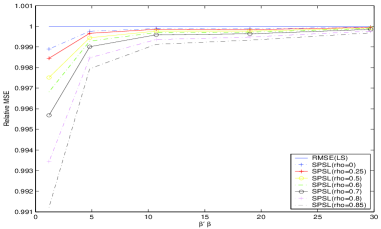
(a) $n=15$, $\sigma=0.1$, $k=3$

(b) $n=15$, $\sigma=0.25$, $k=3$

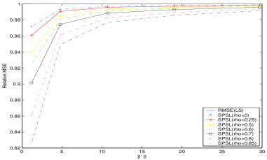
(c) $n=15$, $\sigma=0.5$, $k=3$

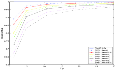
(d) $n=15$, $\sigma=1$, $k=3$

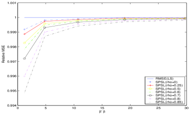
(e) $n=25$, $\sigma=0.1$, $k=3$

(f) $n=25$, $\sigma=0.25$, $k=3$

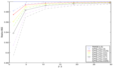
(g) $n=25$, $\sigma=0.5$, $k=3$

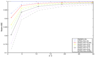
(h) $n=25$, $\sigma=1$, $k=3$

Figure 1: Relative efficiency versus $\beta^{\prime}\beta$

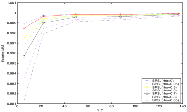
(a) $n=15$, $\sigma=0.1$, $k=3$

(b) $n=15$, $\sigma=0.25$, $k=3$

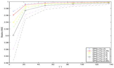
(c) $n=15$, $\sigma=0.5$, $k=3$

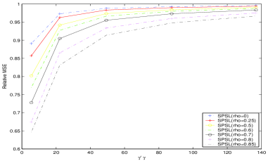
(d) $n=15$, $\sigma=1$, $k=3$

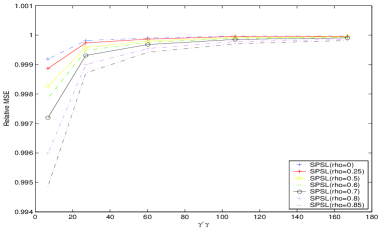
(e) $n=25$, $\sigma=0.1$, $k=3$

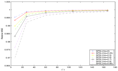
(f) $n=25$, $\sigma=0.25$, $k=3$

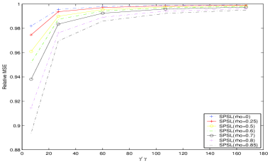
(g) $n=25$, $\sigma=0.5$, $k=3$

(h) $n=25$, $\sigma=1$, $k=3$

Figure 2: Relative efficiency versus $\gamma^{\prime}\gamma$

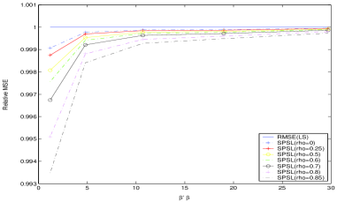
(a) $n=15$, $\sigma=0.1$, $k=4$

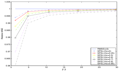
(b) $n=15$, $\sigma=0.25$, $k=4$

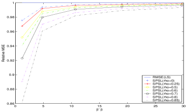
(c) $n=15$, $\sigma=0.5$, $k=4$

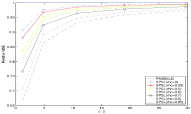
(d) $n=15$, $\sigma=1$, $k=4$

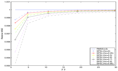
(e) $n=25$, $\sigma=0.1$, $k=4$

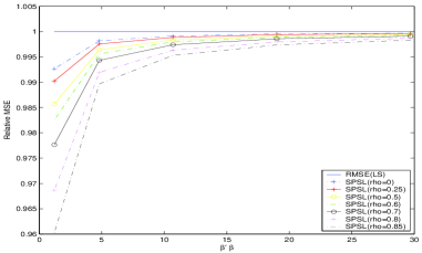
(f) $n=25$, $\sigma=0.25$, $k=4$

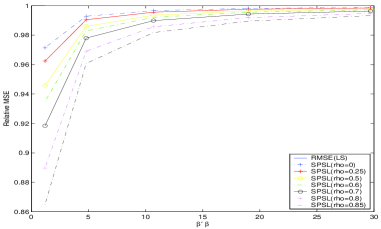
(g) $n=25$, $\sigma=0.5$, $k=4$

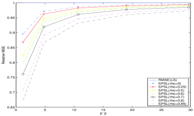
(h) $n=25$, $\sigma=1$, $k=4$

Figure 3: Relative efficiency versus $\beta^{\prime}\beta$

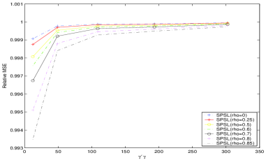
(a) $n=15$, $\sigma=0.1$, $k=4$

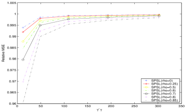
(b) $n=15$, $\sigma=0.25$, $k=4$

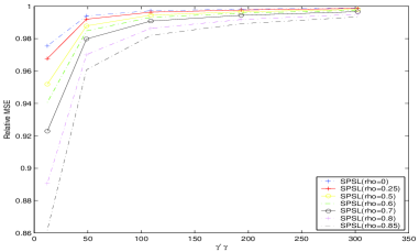
(c) $n=15$, $\sigma=0.5$, $k=4$

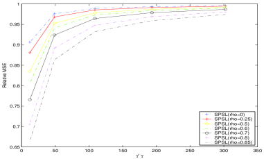
(d) $n=15$, $\sigma=1$, $k=4$

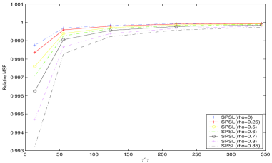
(e) $n=25$, $\sigma=0.1$, $k=4$

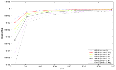
(f) $n=25$, $\sigma=0.25$, $k=4$

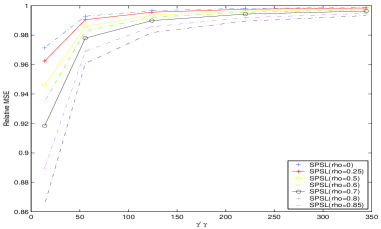
(g) $n=25$, $\sigma=0.5$, $k=4$

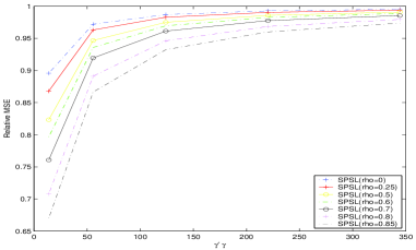
(h) $n=25$, $\sigma=1$, $k=4$

Figure 4: Relative efficiency versus $\gamma^{\prime}\gamma$

More precisely, in this paper, by following the results in Subsection 5.2 of JM (2004), we examine the relative performance of the SPLS estimator as a function of the parameter norms $\beta^{\prime}\beta$ and $\gamma^{\prime}\gamma$, where the parameter vector $\beta$ is chosen such that
$\beta^{\prime}\beta\in\left\{1.2,4.8,10.7,19.0,29.7\right\}$, which are the values used in JM (2004, Figure 3).

For the small sample sizes and $k=3$, the results are presented in Figures 1 and 2. These figures show that, as the norms $\beta^{\prime}\beta$ or $\gamma^{\prime}\gamma$ increase, the risk of the SPSL estimator increases and approaches the risk of the LS estimator. Further, Figures 3-4 show a similar pattern for the case where $k=4$ and/or for the cases of moderate and large sample sizes. This result is in agreement with that given in JM (2004) for the cases where $k\geqslant 5$. Also, these figures confirm the findings in JM (2004) in that the correlation among the $X$ variables increases the relative performance of the SPSL estimator over the LS estimator.

4.2 Data analysis

In this subsection, we illustrate the application of the proposed method to a real data set. The data set consists of a sample of 25 brands of cigarettes (see Mendenhall and Sincich, 1992). For each brand of cigarette, the measurements of weight as well as tar, nicotine, and carbon monoxide content are have been recorded.

The choice of this data set is justified by several health and environmental issues concerning the cigarettes as mentioned by some medical studies. Thus, as explained in Mendenhall and Sincich (1992), ”the United States Surgeon General considers each of these substances hazardous to a smoker’s health”. The authors also mention that ”past studies have shown that increases in the tar and nicotine content of a cigarette are accompanied by an increase in the carbon monoxide emitted from the cigarette smoke”.

Accordingly, in order to illustrate the application of the proposed method, the response variable is taken as the carbon monoxide content, while the three covariates are: $X_{1}$: weight; $X_{2}$: tar content, and $X_{3}$: nicotine content. So, including the intercept, we apply the proposed method to the regression model for which $n=25$ and $k=4$. It should be noticed that, for such a data set whose $k<5$, the result in JM (2004) cannot be used to justify the efficiency of the SPSL over the base estimator. In contrast, the result established in this paper justifies very well the relative efficiency of the SPSL estimator provided that the underlying distribution of the error terms is an elliptically contoured distribution. To give some numerical descriptive measures, the sample mean is 12.5280 for the response variable, and for the covariates, the sample means are 12.2160,   0.8764 and 0.9703 for the weight, tar and nicotine content, respectively. The correlation coefficients between the response and the covariates are shown in Table 1. This table indicates that the weight and the tar content are highly correlated to the response, while the correlation between the nicotine content and the response is modest. Nevertheless, the correlation coefficients are statistically significant at the 5 % level. Further, the covariates seem pairwise correlated at significance level 5 %.

Table 1: Correlation between covariates and response variables (p-value in parentheses)

	carbon monoxide	Weight	Tar content	Nicotine content
carbon monoxide	1	0.9575	0.9259	0.4640
	(-)	(0.0000)	(0.0000 )	(0.0195)
Weight	0.9575	1	0.9766	0.4908
	(0.0000)	(-)	(0.0000 )	(0.0127)
Tar content	0.9259	0.9766	1	0.5002
	(0.0000 )	(0.0000)	(-)	(0.0109)
Nicotine content	0.4640	0.4908	0.5002	1
	(0.0195)	(0.0127 )	( 0.0109 )	(-)

By applying the method, we obtain the point estimates based on the LS and SPSL estimators as reported in Table 2. To asses the performance of the estimators, we compute the mean squared error based on a bootstrap method with 5000 replications. The relative efficiency of the estimators is given in Table 3.

Table 2: Point Estimates

Parameter	LS	SPSL
Intercept	3.2022	3.9325
Weight	0.9626	0.9645
Tar	-2.6317	-1.3262
Nicotine	-0.1305	0.8983

Table 3: Relative efficiency (Bootstrap)

Estimator	LS	SPSL
Relative efficiency	1	0.7578

From Table 3, one can clearly see that the relative efficiency of the SPSL estimstor is less than 1, that is the relative efficiency of the base estimator. This illustrates that SPSL dominates the base estimator.

5 Conclusion

In order to conclude, let us first recall that the main result in JM (2004) gives a sufficient condition for the Stein rule (SR)-type estimator to dominate the base estimator. In this paper, we provided more refined inequalities and bounds which are used in establishing this result in its full generality. Namely, we generalized in four ways the result in JM (2004) which gives a sufficient condition for the Stein rule (SR)-type estimator to dominate the base estimator. To this end, we provided an alternative and a versatile approach for establishing the dominance result in its full generality. In particular, we proved theoretically that the nonzero correlation does not change the condition for the risk dominance of the SR estimator. The impact of this result is that, unlike the method in JM (2004), our method is also applicable to a wide range of regression models, including, for instance, the quadratic or cubic regressions, where the number of regressors is less than 5. In addition, we relax the condition of normality of the sampling distribution of the base estimator. We also generalize the method in JM (2004) to the case where the variance-covariance matrix of the base estimator and the restricted estimator may be singular. The significance of this finding is that our method is also efficient in the case where the past statistical investigations may have established that some regression coefficients are not statistically significant while a field specialist believes that the nonsignificant explanatory variables are important. From the practical point of view, we evaluate numerically the relative efficiency of a data-based semiparametric Stein-like (SPSL) estimator. The simulation studies corroborate this theoretical finding that the sufficient condition, for the SPSL to dominate the LS estimator ($k\geqslant 3$), holds also regardless of the correlation factor. Nevertheless, Figures 1-8 show that the correlation may amplify the risk dominance of the SPSL. Finally, the proposed method is applied to the Cigarette dataset, produced by USA Federal Trade Commission, for which $k=4$. An interesting result is that, by using a bootstrap method, we see that the SPSL dominates the base estimator. This finding is in agreement with the theoretical result proved in the present paper.

Appendix A Appendix

Proposition A.1.

Let $\bm{C}$ be a $m\times m$-symmetric matrix. Then,
$\left|x^{\prime}Cx\right|\leqslant\max\{|\lambda_{1}(\bm{C})|,|\lambda_{2}(\bm{C})|,\dots,|\lambda_{m}(\bm{C})|\}x^{\prime}x$, for all $m$-column vector $x$.

Proof.

Since the matrix $\bm{C}$ is symmetric, there exist orthogonal matrix $\bm{Q}$ such that

$\bm{Q}^{\prime}\bm{C}\bm{Q}=\bm{D}=\textrm{ diag}\left(\lambda_{1}(\bm{C}),\lambda_{2}(\bm{C}),\dots,\lambda_{m}(\bm{C})\right)$. Therefore,

$$x^{\prime}\bm{C}x=x^{\prime}\bm{Q}\bm{Q}^{\prime}\bm{C}\bm{Q}\bm{Q}^{\prime}x=y^{\prime}\bm{D}y=\sum_{i=1}^{m}\lambda_{i}(\bm{C})y_{i}^{2},\quad{}y=\bm{Q}^{\prime}x=\left(y_{1},y_{2},\dots,y_{m}\right)^{\prime}.$$

Therefore,

$$|x^{\prime}\bm{C}x|=|\sum_{i=1}^{m}\lambda_{i}(\bm{C})y_{i}^{2}|\leqslant\sum_{i=1}^{m}|\lambda_{i}(\bm{C})|y_{i}^{2}\leqslant\max\{|\lambda_{1}(\bm{C})|,|\lambda_{2}(\bm{C})|,\dots,|\lambda_{m}(\bm{C})|\}\sum_{i=1}^{m}y_{i}^{2}$$

$$\leqslant\max\{|\lambda_{1}(\bm{C})|,|\lambda_{2}(\bm{C})|,\dots,|\lambda_{m}(\bm{C})|\}y^{\prime}y=\max\{|\lambda_{1}(\bm{C})|,|\lambda_{2}(\bm{C})|,\dots,|\lambda_{m}(\bm{C})|\}x^{\prime}x,$$

this completes the proof. ∎

Corollary A.2.

Let $\bm{C}$ be a $m\times m$-matrix. Let $x$ and $y$ $m-$column vectors. Then, we have

$\left|x^{\prime}\bm{C}x\right|\leqslant\frac{1}{2}\,\max\{|\lambda_{1}(\bm{C}+\bm{C}^{\prime})|,|\lambda_{2}(\bm{C}+\bm{C}^{\prime})|,\dots,|\lambda_{m}(\bm{C}+\bm{C}^{\prime})|\}x^{\prime}x$, and

$\left|y^{\prime}\bm{C}x\right|\leqslant\frac{1}{2}\,\max\{|\lambda_{1}(\bm{B}_{0})|,|\lambda_{2}(\bm{B}_{0})|,\dots,|\lambda_{2m}(\bm{B}_{0})|\}(x^{\prime}x+y^{\prime}y)$, where $\bm{B}_{0}=\left(\begin{array}[]{cc}\bm{0}&\bm{C}^{\prime}\\ \bm{C}&\bm{0}\\ \end{array}\right).$

Proof.

Since $x^{\prime}\bm{C}x$ is a real number, we have $x^{\prime}\bm{C}x=\frac{1}{2}\,x^{\prime}(\bm{C}+\bm{C}^{\prime})x$. Therefore, since $\bm{C}+\bm{C}^{\prime}$ is a symmetric matrix, the first statement follows directly from Proposition A.1. To prove the second statement, note that $y^{\prime}\bm{C}x$ can be rewritten as

$$y^{\prime}\bm{C}x=(x^{\prime},y^{\prime})\left[(\bm{0},\,\bm{C}^{\prime})^{\prime}\quad{}\vdots\quad{}\bm{0}\right]\left(x^{\prime},\,y^{\prime}\right)^{\prime}.$$

The rest of the proof follows from the first statement. ∎

Proof of Proposition 3.1.

Under Assumption $(\mathcal{H})$, there exists $q_{\scriptscriptstyle 0}>0$ such that
$|h(\hat{\beta},\tilde{\beta})|\leqslant q_{\scriptscriptstyle 0}\Big{/}\|\hat{\beta}-\tilde{\beta}\|^{2}$. Then, we have

$$|\eta(h)|\leqslant\textrm{E}\left(|h(\hat{\beta},\tilde{\beta})||\hat{\beta}-\beta|\right)\leqslant q_{\scriptscriptstyle 0}\textrm{E}\left(|\hat{\beta}-\beta|\Big{/}\|\hat{\beta}-\tilde{\beta}\|^{2}\right),$$

and then, by using (2.5) and (3.5), we get

$$\textrm{E}\left(|\hat{\beta}-\beta|/\|\hat{\beta}-\tilde{\beta}\|^{2}\right)=\textrm{E}\left(|U^{\prime}_{1}PZ|\,\Big{/}Z^{\prime}RZ\right),$$

this proves the first statement of the proposition. Further, we have

$$|\omega(h)|=\textrm{E}\left(h^{2}(\hat{\beta},\tilde{\beta})\|\hat{\beta}-\tilde{\beta}\|^{2}\right)\leqslant q^{2}_{\scriptscriptstyle 0}\textrm{E}\left(1\,\Big{/}\|\hat{\beta}-\tilde{\beta}\|^{2}\right),$$

and then, by using (2.5) and (3.5), we get

$$\textrm{E}\left(1\,\Big{/}\|\hat{\beta}-\tilde{\beta}\|^{2}\right)=\textrm{E}\left(1\,/Z^{\prime}RZ\right)=\omega,$$

this completes the proof. ∎

Proof of Proposition 3.2.

Let $W=\left(Z^{\prime},U^{\prime}_{1}\right)^{\prime}$. We have

$$\textrm{E}\left\{\left(|U_{1}^{\prime}\bm{P}Z|\,\big{/}(Z^{\prime}\bm{R}Z)\right)\mathbb{I}_{\left\{\|W\|\leqslant\alpha\right\}}\right\}=\textrm{E}\left\{\left(|W^{\prime}\bm{F}W|\,\big{/}(Z^{\prime}\bm{R}Z)\right)\mathbb{I}_{\left\{\|W\|\leqslant\alpha\right\}}\right\},$$ (A.1)

where $F$ is defined in (3.13). By using Corollary A.2, we get

$$\textrm{E}\left\{\frac{|W^{\prime}\bm{F}W|}{Z^{\prime}\bm{R}Z}\mathbb{I}_{\left\{\|W\|\leqslant\alpha\right\}}\right\}\leqslant\frac{1}{2}\,\psi_{1}\,\textrm{E}\left\{\frac{1}{Z^{\prime}\bm{R}Z}\|W\|^{2}\mathbb{I}_{\left\{\|W\|\leqslant\alpha\right\}}\right\}\leqslant\frac{1}{2}\,\psi_{1}\,\textrm{E}\left\{\frac{\alpha^{2}}{Z^{\prime}\bm{R}Z}\mathbb{I}_{\left\{\|W\|\leqslant\alpha\right\}}\right\},$$

which gives

$$\textrm{E}\left\{\left(|W^{\prime}\bm{F}W|\,/(Z^{\prime}\bm{R}Z)\right)\,\mathbb{I}_{\left\{\|W\|\leqslant\alpha\right\}}\right\}\leqslant\alpha^{2}\,\psi_{1}\,\textrm{E}\left\{1/(Z^{\prime}\bm{R}Z)\right\}\,\big{/}2\leqslant\alpha^{2}\,\psi_{1}\,\omega\,\big{/}2,$$ (A.2)

and the proof is completed. ∎

Proof of Proposition 3.3.

We have,

$$\textrm{E}\left\{\frac{|W^{\prime}\bm{F}W|}{Z^{\prime}\bm{R}Z}\,\mathbb{I}_{\left\{\|W\|>\alpha\right\}}\right\}\leqslant\textrm{E}\left\{\left(|W^{\prime}\bm{F}W|\,\big{/}(Z^{\prime}\bm{R}Z)\right)\,\mathbb{I}_{\left\{\|Z\|^{2}>\frac{\alpha^{2}}{2}\right\}}\right\}\leqslant\frac{2}{\alpha^{2}}\textrm{E}\left\{|W^{\prime}\bm{F}W|\,\frac{\|Z\|^{2}}{Z^{\prime}\bm{R}Z}\right\}.$$

By Courant’s Theorem, we have the inequality

$$1/\max\{\lambda_{1}(\bm{R}),\lambda_{2}(\bm{R}),\dots,\lambda_{k}(\bm{R})\}\leqslant\|Z\|^{2}/(Z^{\prime}\bm{R}Z)\leqslant 1/\psi_{0},$$

which gives

$$\textrm{E}\left\{\left(|W^{\prime}\bm{F}W|\,\big{/}(Z^{\prime}\bm{R}Z)\right)\,\mathbb{I}_{\left\{\|Z\|^{2}>\alpha^{2}/2\right\}}\right\}\leqslant 2\,\textrm{E}\left\{|W^{\prime}\bm{F}W|\right\}\,\big{/}(\alpha^{2}\,\psi_{0}).$$ (A.3)

Further, by using Corollary A.2, we get

$$\textrm{E}\left\{|W^{\prime}\bm{F}W|\right\}\leqslant\max\{|\lambda_{1}(\bm{F}+\bm{F}^{\prime})|,|\lambda_{2}(\bm{F}+\bm{F}^{\prime})|,\dots,|\lambda_{2m}(\bm{F}+\bm{F}^{\prime})|\}\textrm{E}(W^{\prime}W)\,\big{/}2.$$ (A.4)

Note that $\bm{F}+\bm{F}^{\prime}=\bm{B}$ and $W\sim\mathcal{N}_{2k}\left(\left(\begin{array}[]{c}\mu\\ \bm{0}\\ \end{array}\right),\left(\begin{array}[]{cc}\bm{I}_{k}&(\bm{A}-\bm{\Sigma})(\bm{P}^{-1})^{\prime}\\ \bm{P}^{-1}(\bm{A}-\bm{\Sigma}^{\prime})&\bm{A}\\ \end{array}\right)\right)$. Then, $\textrm{E}(W^{\prime}W)=\textrm{trace}(\bm{A})+k+\mu^{\prime}\mu$, and then,

$$\textrm{E}\left\{|W^{\prime}\bm{F}W|\right\}\leqslant\,\psi_{1}\left[\textrm{trace}(\bm{A})+k+\mu^{\prime}\mu\right]\,\big{/}2.$$ (A.5)

By combining (A.3), (A.4) and (A.5), we get the statement of the proposition, which completes the proof. ∎

Proposition A.3.

Suppose that Assumptions $(\mathcal{H}_{1})$ and $(\mathcal{H}_{2})$ hold. Then, under normality, $\omega(h)<\infty$ provided that $q\geqslant 3$.

Proof.

We have $\omega(h)=\textrm{E}\left[h^{2}(\hat{\beta},\tilde{\beta})\left\|\hat{\beta}-\tilde{\beta}\right\|^{2}\right]$, and then, under Assumption $(\mathcal{H}_{1})$, there exist $q_{0}$ such that

$$\omega(h)\leqslant q_{0}\textrm{E}\left[1\Big{/}\left\|\hat{\beta}-\tilde{\beta}\right\|^{2}\right]\leqslant q_{0}\textrm{trace}(\bm{\Lambda}\bm{\Xi}\bm{\Lambda})\textrm{E}\left[1\Big{/}\left(\hat{\beta}-\tilde{\beta}\right)^{\prime}\bm{\Lambda}\bm{\Xi}\bm{\Lambda}\left(\hat{\beta}-\tilde{\beta}\right)\right].$$

Further, by using Theorem 5.1.3 in Mathai and Provost (1992, p. 199), we have
$\left(\hat{\beta}-\tilde{\beta}\right)^{\prime}\bm{\Lambda}\bm{\Xi}\bm{\Lambda}\left(\hat{\beta}-\tilde{\beta}\right)\sim\chi^{2}_{q}\left(\gamma^{\prime}\bm{\Lambda}\bm{\Xi}\bm{\Lambda}\gamma\right)$ and then,

$$\textrm{E}\left[1\Big{/}\left(\hat{\beta}-\tilde{\beta}\right)^{\prime}\bm{\Lambda}\bm{\Xi}\bm{\Lambda}\left(\hat{\beta}-\tilde{\beta}\right)\right]=\textrm{E}\left[\chi^{-2}_{q}\left(\gamma^{\prime}\bm{\Lambda}\bm{\Xi}\bm{\Lambda}\gamma\right)\right]<1/(q-2).$$

Hence, $\omega(h)<q_{0}\textrm{trace}(\bm{\Lambda}\bm{\Xi}\bm{\Lambda})/(q-2)<+\infty$ provided that $q\geqslant 3$, this completes the proof. ∎

Proof of Theorem 3.10.

We have

$$\eta(h)=\textrm{E}\left[h(\hat{\beta},\tilde{\beta})\left(\hat{\beta}-\beta\right)^{\prime}\left(\hat{\beta}-\tilde{\beta}\right)\right],$$

and this gives

$$\eta(h)=\textrm{E}\left[h(\hat{\beta},\tilde{\beta})\left\|\hat{\beta}-\tilde{\beta}\right\|^{2}\right]+\textrm{E}\left[h(\hat{\beta},\tilde{\beta})\left(\tilde{\beta}-\beta\right)^{\prime}\left(\hat{\beta}-\tilde{\beta}\right)\right].$$

Then, by the triangular inequality,

$$|\eta(h)|\leqslant\left|\textrm{E}\left[h(\hat{\beta},\tilde{\beta})\left\|\hat{\beta}-\tilde{\beta}\right\|^{2}\right]\right|+\left|\textrm{E}\left[h(\hat{\beta},\tilde{\beta})\left(\tilde{\beta}-\beta\right)^{\prime}\left(\hat{\beta}-\tilde{\beta}\right)\right]\right|.$$

Then, by using Jensen’s inequality and Assumption $(\mathcal{H}_{1})$, we get

$$|\eta(h)|\leqslant q_{0}+\left|\textrm{E}\left[h(\hat{\beta},\tilde{\beta})\left(\tilde{\beta}-\beta\right)^{\prime}\left(\hat{\beta}-\tilde{\beta}\right)\right]\right|.$$

Further, since $\left(\tilde{\beta}-\beta\right)$ and $\left(\hat{\beta}-\tilde{\beta}\right)$ are independent, and since, by Assumption $(\mathcal{H}_{2})$, $h(\hat{\beta},\tilde{\beta})$ is a measurable function of $\hat{\beta}-\tilde{\beta}$ only, we have

$$|\eta(h)|\leqslant q_{0}+\left|\gamma^{\prime}\textrm{E}\left[h(\hat{\beta},\tilde{\beta})\left(\hat{\beta}-\tilde{\beta}\right)\right]\right|.$$

Then, by Cauchy-Schwarz inequality,

$$|\eta(h)|\leqslant q_{0}+\left\|\gamma\right\|\left\{\textrm{E}\left[h^{2}(\hat{\beta},\tilde{\beta})\left\|\hat{\beta}-\tilde{\beta}\right\|^{2}\right]\right\}^{1/2}=q_{0}+\left\|\gamma\right\|\omega^{1/2}(h).$$

Therefore, the proof follows from Proposition A.3. ∎

References

- [1] Abdous, B., Genest, C., and R�millard, B. (2004). Dependence properties of meta-elliptical distributions. In: Duchesne, P. and R�millard, B. (Eds.), Statistical Modeling and Analysis for Complex Data Problems, Kluwer.
- [2] Ashton, K. G., Burke, R. L., and Layne, J. N. (2007). Geographic variation in body and clutch of gopher tortoises. Copeia, 2007, 355–363.
- [3] Bingham, N. H., and Kiesel, R. (2001). Semi-parametric modelling in finance: theoretical foundations. Quantitative Finance, 1, 1–10.
- [4] Bock, B. E. (1975). Minimax estimators of the mean of a multivariate normal distribution. Annals of Statistics, 3, 209–218.
- [5] Chmielewski, M. A. (1981). Elliptically Symmetric Distributions: A Review and Bibliography. International Statistical Review, 49, 1, 67–74.
- [6] Douglas, P., and Cobb, C. (1928). A theory of production. American Economic Review, 18.
- [7] Fernandez-Juricic, E., Sanz, R., and Rodriguez-Prieto, I. (2003). Testing the risk-disturbance hypothesis in fragmented landscape: non-linear responses of house sparrows to humans. Condor, 105, 316–326.
- [8] Furman, E., and Landsman, Z. (2006). Tail variance premium with applications for elliptical portfolio of risks. Astin Bulletin, 36, 2, 433–462.
- [9] Gupta, A. K., and Varga, T. (1995). Normal mixture representations of matrix variate elliptically contoured distributions,Sankhy, 57, 68–78.
- [10] Hossain, S., Doksum, K. A., and Ahmed, S. E. (2009). Positive shrinkage, improved pretest and absolute penalty estimators in partially linear models. Linear Algebra and its Applications, 430, 2749–2761.
- [11] James, W., Stein, C. (1961). Estimation with quadratic loss. Proc. Fourth Berkeley Symp. Math. Statist. Prob., 1, 361–379.
- [12] Judge, G. G., and Bock, M. E. (1978). The statistical implication of pre-test and Stein-rule estimators in econometrics. Amsterdam, North Holland.
- [13] Judge, G. G., and Mittelhammer, R. C. (2004). A Semiparametric Basis for Combining Estimation Problems under Quadratic Loss. Journal of the American Statistical Association (JASA), 99, 466, 479–487.
- [14] Landsman, Z. M., and Valdez, E. A. (2003). Tail conditional expectations for elliptical distributions. North American Actuarial Journal, 7, 4,55–123.
- [15] Liu, J. S., Cheung, W., and Wong, H. (2009). Predictive inference for singular multivariate elliptically contoured distributions. Journal of Multivariate Analysis, 100, 1440–1446.
- [16] Mathai, A.M. and Provost, S. B. (1992). Quadratic Forms in Random Variables (Statistics: A Series of Textbooks and Monographs). Marcel Dekker, Inc., New York.
- [17] Mendenhall, W., and Sincich, T. (1992). Statistics for Engineering and the Sciences ( ed.). New York: Dellen Publishing Co.
- [18] Morris, C. N., and Lysy, M. (2012). Shrinkage estimation in multilevel normal models. Statistical Science, 27, 115–134.
- [19] Nkurunziza, S., and Ahmed, S. E. (2010). Shrinkage Drift Parameter Estimation for Multi-factor Ornstein-Uhlenbeck Processes. Applied Stochastic Models in Business and Industry, 26, 2, 103–124.
- [20] Nkurunziza, S. (2011). Shrinkage Strategy In Stratified Random Sample Subject To Measurement Error. Statistics and Probability Letters, 81, 317–325.
- [21] Nkurunziza, S. (2013). The bias and risk functions of some Stein-rules in elliptically contoured distributions. Mathematical Methods of Statistics, 22, 1, 70–82.
- [22] Nkurunziza, S., and Chen, F. (2013). On extension of some identities for the bias and risk functions in elliptically contoured distributions. Journal of Multivariate Analysis, 122, 190–201.
- [23] Provost, S. B., and Cheong, Y. H. (2000). On the distribution of linear combinations of the components of a Dirichlet random vector. Can. J. Stat., 28, 2, 417–425.
- [24] Saleh, A. K. Md. (2006). Theory of Preliminary Test and Stein-Type Estimation with Applications. John Wiley & Sons, Inc., Hoboken, New Jersey.
- [25] Tan, Z. (2015). Improved Minimax Estimation of a Multivariate Normal Mean under Heteroscedasticity. Bernoulli Journal, 21, 1, 574–603.