Line and Continuum Variability in Active Galaxies

Y. E. Rashed,^1,2 A. Eckart,^1,3 M. Valencia-S.,¹ M. García-Marín,¹ G. Busch,¹ J. Zuther,¹ M. Horrobin,¹ and H. Zhou^4,5
¹I. Physikalisches Institut, Universität zu Köln, Zülpicher Straße 77, 50937 Köln, Germany
²Department of Astronomy, Faculty of Science, University of Baghdad, 10071 Baghdad - Aljadirya, Iraq
³Max-Planck-Institut für Radioastronomie, Auf dem Hügel 69, 53121 Bonn, Germany
⁴Key laboratory for Research in Galaxies and Cosmology, Department of Astronomy,
The University of Sciences and Technology of China, Chinese Academy of Sciences, Hefei, Anhui 230026, China
⁵Polar Research Institute of China, Jinqiao Rd. 451, Shanghai 200136, China; zhouhongyan@pric.gov.cn yasir@ph1.uni-koeln.de

(Accepted 2015 September 3. Received 2015 August 24; in original form 2015 July 3)

Abstract

We compared optical spectroscopic and photometric data for 18 AGN galaxies over 2 to 3 epochs, with time intervals of typically 5 to 10 years. We used the Multi-Object Double Spectrograph (MODS) at the Large Binocular Telescope (LBT) and compared the spectra to data taken from the SDSS database and the literature. We find variations in the forbidden oxygen lines as well as in the hydrogen recombination lines of these sources. For 4 of the sources we find that, within the calibration uncertainties, the variations in continuum and line spectra of the sources are very small. We argue that it is mainly the difference in black hole mass between the samples that is responsible for the different degree of continuum variability. In addition we find that for an otherwise constant accretion rate the total line variability (dominated by the narrow line contributions) reverberates the continuum variability with a dependency $\Delta L_{line}\propto(\Delta L_{cont.})^{\frac{3}{2}}$ . Since this dependency is prominently expressed in the narrow line emission it implies that the luminosity dominating part of the narrow line region must be very compact with a size of the order of at least 10 light years. A comparison to literature data shows that these findings describe the variability characteristics of a total of 61 broad and narrow line sources.

keywords:

Galaxies: Active – Variability.

^†^†pagerange: Line and Continuum Variability in Active Galaxies–18^†^†pubyear: 0000

1 Introduction

Seyfert galaxies and quasars are the main types of active galactic nuclei (AGNs) in which the nuclei are dominated by a very powerful electromagnetic emitter. Seyfert nuclei are 10 to 100 times brighter than the host galaxies they reside in. Thus, these nuclei are responsible for most activity that occurs within the central 10-100 pc of these hosts.

Seyfert galaxies can show a wide variety of forbidden and permitted emission lines, which can have widths up to $\sim 10\ 000\,\mathrm{km}\,\mathrm{s}^{-1}$ via Doppler broadening. Depending on the width of the emission lines, one distinguishes between two main categories, Seyfert-1 (S1) and Seyfert-2 (S2): S2 galaxies show only narrow lines ( $\lesssim 1000\,\mathrm{km}\,\mathrm{s}^{-1}$ ), while S1 show additional broad components ( $\lesssim 10\ 000\,\mathrm{km}\,\mathrm{s}^{-1}$ ) in the permitted lines. The emission lines are commonly believed to stem from the “broad line region” (BLR) and the “narrow line region” (NLR), which are gas clouds orbiting a central super-massive black hole (SMBH) at very high velocities. The gas clouds are excited by continuum radiation produced by an accretion disk of material infalling around the central SMBH. According to the unified model (e.g., Antonucci, 1993; Urry & Padovani, 1995), the existence of S1 galaxies which have broad and narrow lines, and S2 galaxies which only have narrow lines, can be attributed to inclination effects. One possible scenario is a dusty torus which surrounds the accretion disk and BLR, obscuring the emission from the BLR if the galaxy is observed with a viewing angle parallel to the torus plane.

Narrow-line Seyfert-1 (NLS1) galaxies are S1 galaxies that have broad components with comparably narrow widths ( $\lesssim 2000\,\mathrm{km}\,\mathrm{s}^{-1}$ ). From an observational point of view it appears that there are two main differences between S2 and NLS1 galaxies. The first one is that NLS1 objects have Fe ii in their spectra (which originate in the BLR), which is absent in the S2 spectra (Giannuzzo & Stirpe, 1996). The second is that some NLS1 sources show strong lines of highly ionized iron in their spectra e.g. [Fe vii] $\lambda 5721$ Å and [Fe x] $\lambda 6375$ Å (Osterbrock, 1985; Osterbrock & Pogge, 1985), these lines are rare and not typical for the S2 spectra.

AGNs are characterized by variability at almost all wavelengths (Peterson, 2001). Studying the variability on all time scales is a very useful approach to investigate and understand the physical properties of AGNs, there are many systematic studies on the variability of AGN using spectroscopic and photometric observations. Photometric measurements have been used to study the variability, despite the fact that bright line emission is located within the corresponding passband (Vanden Berk et al., 2004). Studying the spectral variability both in line and in continuum emission has become an important topic that may help to outline differences between different Seyfert source classes. Variability may indicate how the active galactic nuclei (AGN) affect the regions surrounding them (i.e. the BLR and NLR) and how these regions change as a function of time. Many interesting results have been obtained from AGN samples of various types and sizes. A noted one is the anti-correlation between the continuum luminosity and variability, which was first reported by Angione & Smith (1972). Later additional information on this effect was provided by Hook et al. (1994); Zuo et al. (2012, 2013). Additionally, other authors (Cid Fernandes & Sodre, 2000; Meusinger & Weiss, 2013) have clarified that this anti-correlation can qualitatively be described via the standard accretion disk model, proposing that the variability is caused via the variation of the accretion rate.

Since spectroscopic studies can be very time consuming, there are only a few detailed, spectroscopy-based comparative studies on the variability of AGNs. They either concentrate on reverberation mapping analysis of extensively observed sources (e.g., Kaspi et al., 2007) or depend on just a few epochs of spectroscopic observations (e.g., Wilhite et al., 2005). Multi epoch spectroscopy observations have advantages compared to photometric observations, as they allow us to study the continuum and line emission at the same time. Excepting regions of high emission line density, these observations also allow us to extract the underlying continuum spectrum over a broad wavelength range and to study the spectral shape of the lines and the line spectrum in general. The emission line spectra then allow us to study the BLR and NLR regions surrounding the compact variable continuum nuclei.

Examples of extensive investigations on the variability in Seyferts and quasars concentrating on the continuum and the fluxes of the emission lines are, e.g., Peterson et al. (1984); Peterson & Gaskell (1986); Peterson et al. (1998); Guo & Gu (2014). While the BLR lines are found to reverberate the continuum variability on time scales of days, there are also a few reports of long term line variability in the NLR region: Based on a time coverage of 8 years Clavel & Wamsteker (1987) find for 3C390.3 that the NLR is photoionized and reverberates the continuum flux. They set an upper limit of 10 light years for the size of the NLR. Based on a time coverage of 5 years Peterson et al. (2013) find for the S1 galaxy NGC 5548 that the [O III] $\lambda\lambda$ 4959, 5007 emission-line flux varies with time and give a size estimate of 1-3 pc (i.e. 3-9 light years). There is a clear connection between the continuum and line variability. For instance, Peterson et al. (1984) found that for $\sim$ 73% of the cases they studied, there is variability in the $\mathrm{H\beta}$ line flux corresponding to the changes in the continuum. On the other hand, in the same project, they found that this correlation is not true for the sources if the continuum changes by more than $\sim$ 70%. They suggest that for cases in which the $\mathrm{H\beta}$ flux does not correspond to the continuum, light travel time effects may have to be included. Furthermore, there is still no absolute conclusion on the correlation between the emission lines width and the line luminosity. An anti-correlation was found in a sample of 85 quasars by Brotherton et al. (1994), with single-epoch spectroscopic data. On the other hand Wilhite et al. (2005) found that there is a correlation between the emission lines width and the line luminosity. They conclude this from a spectroscopic sample of 315 quasars.

2 Paper outline and sample selection

In this paper we investigate the continuum and narrow line variability of a small sample of objects over a good fraction of a decade. The spectra cover a major fraction of the entire optical wavelength domain from the blue to the red, including several prominent lines, and also have an appreciable signal to noise ratio in the continuum emission. For such a study it is essential that the spectra are well calibrated such that they can be compared to each other. It is also important to correct for iron emission in order to extract proper values for the line luminosities of species other than iron. As the data has been taken with different instruments and different effective apertures on the sky it is furthermore essential to make sure that aperture effects, which may occur due to slit losses, or from extended and spatially resolved line or continuum emission from the host galaxies, do not contaminate the results of the variability assessment. In the literature one rarely finds appropriately calibrated or sufficiently described data sets that are suitable for long term variability studies. Hence we made the effort to collect and combine a representative data set. This comprises a total of 18 sources (see summary in Sec. 6.1). For 8 objects we obtained and/or performed the detailed analysis over the available optical wavelength range using data from the LBT and other observatories (see Sect. 3.1 and Tab. LABEL:all_sources1). These 8 sources were selected on the basis of their observability (given the allocated observing dates), their brightness (such that with the chosen integration times a decent signal to noise could be reached that allows comparison to public survey data), and the fact that a previous first epoch spectrum had been taken typically 5-10 years ago. Based on their [MgII] absorption, the 8 sources include 3 loBAL QSOs. However, given that their spectra also contain prominent broad emission lines, we decided to include them in the characterization of the BLQSOs/Sy1 variability. In order to reach our goal of studying the difference in the variability properties of BLQSOs/Sy1 and NLSy1/S2 galaxies, it was clear that literature data on additional sources had to be added to enlarge the statistical basis. Hence, all conclusions drawn in this paper are based on the resulting larger samples of sources.

For 5 sources (3 NLS1 and only 2 BLS1) we obtained spectroscopic information from the literature. For a further 5 sources (2 NLS1 and 3 BLS1) we found sparser but suitable line and continuum information in the literature. A detailed description of the observations and data reduction is given in Sect. 3, followed by a description of the methods used for our analysis in Sect. 4. In Sect. 5 we present the results for all galaxies that we used in our study.

The sample also comprises sources with a range of identifications. For the purpose of this investigation we combined sources that show very prominent broad emission lines, i.e. Broad Line Seyfert 1 and Quasi Stellar Objects (in the following BLS1 and QSO) in addition to the narrow lines on which our investigation focuses. We also put Seyfert 2 and Narrow Line Seyfert 1 (S2¹¹1One of our sample sources is a composite HII/S2 galaxy - but see discussion in Sect. 5.1 and NLS1) in one group as their spectra are dominated by narrow line emission. An additional justification for this combination is based on the fact that while the unified model of Seyfert galaxies suggests that there are hidden broad-line regions (HBLRs) in all Seyfert 2 galaxies, there is increasing evidence for the presence of a subclass of Seyfert 2 sources lacking these HBLRs (Zhang & Wang, 2006; Haas et al., 2007). In these cases one cannot exclude that we have a free sight to the nucleus despite of the fact that the source is classified as a S2 galaxy. We also refer here to the discussion in the review on NLS1 galaxies by Komossa (2008). Hence, if one classifies sources based on the presence of absence of pronounced broad line emission, then S2 and NLS1 may be more comparable to each other than e.g. BLS1 with NLS1 sources. In the discussion in Sect. 6 and 6.1 we analyze the observed degrees of continuum and narrow line variability. In retrospect we found that the above described combination of sources is indeed justified by their different variability characteristics.

Clearly, at some point such an investigation needs to be performed using larger samples. Since an appropriate baseline for variability studies is several years, such an effort needs time and can only be provided in the near future. However, to study first order effects, the number of sources needs to be only sufficiently large to separate the median or mean properties within the statistical uncertainties. As we outline in the paper, this can already be done with the current, representative sample presented here. In fact, the interpretation we present in Sect. 6.2 may also be taken as a prediction of the effect that the degree of the continuum variability is indeed reverberated by the degree of narrow line variability. This prediction was motivated by the results of the analysis of the small but representative sample we present in this paper. A conclusion is given in Sect. 7.

3 Observation and Data Reduction

In this section, we describe the telescopes and instruments we used for the spectroscopic observations and the procedures followed for the data reduction. We also use complementary data from the literature and public archives like the seventh data release of the SDSS (Abazajian et al., 2009).

3.1 Multi-Object Double Spectrograph (MODS)

For our observations we used the MODS spectrograph at the Large Binocular Telescope (LBT) (Pogge et al., 2010, 2012). The LBT is located on Mount Graham in the Pinaleno Mountains southeastern Arizona, USA. The MODS spectrograph consists of a pair of identical double beam blue & red optimized optical spectrographs (MODS1 & MODS2) which work as individual spectrographs. The instrument can be used for imaging, long-slit, and multi-object spectroscopy. The charge-coupled device (CCD) detector of MODS is an e2vCCD231-68 $8k\times 3k$ with a 15 $\mu$ m pixel pitch.

We use MODS in long-slit mode with a slit width of 0 $\aas@@fstack{\prime\prime}$ 8. The spectrograph operates between 3200-10500 Å with a spectral resolution of R= $\lambda/\delta\lambda\approx 2000$ (i.e., $\sim 150\ \mathrm{km}\ \mathrm{s}^{-1}$ ) where the full spectral range of the grating spectroscopy is split into a blue and red channel, which are 3200-6000 Å (blue) and 5000-10500 Å (red). All objects which we targeted with our LBT observing program are listed in Tab. LABEL:all_sources1.

3.2 The Sloan Digital Sky Survey

The Sloan Digital Sky Survey (SDSS) is a sensitive photometric and spectroscopic public survey which started science operation in May 2000 and covers $10^{4}$ square degrees of the celestial sphere in the northern sky (Stoughton et al., 2002). The survey uses a dedicated 2.5-m wide-angle optical telescope mounted at Apache Point Observatory in New Mexico, United States (Latitude 32°46′49 $\aas@@fstack{\prime\prime}$ 30 N, Longitude 105°49′13 $\aas@@fstack{\prime\prime}$ 50 W, Elevation 2788m). This instrument provides images and photometric parameters in five bands ( $u$ , $g$ , $r$ , $i$ , and $z$ ) with an average seeing of 1 $\aas@@fstack{\prime\prime}$ 5 and down to a limiting magnitude of $\sim 22.2$ in $r$ band. Spectroscopy of selected objects is done through 3″fibers with calibration uncertainties of the order of 2%. The spectral resolution R of the instrument is about $R\sim 2000$ , covering a wavelength range between 3800 and 9200 Å.

In this research we used the SDSS active galaxies (Seyfert & Quasar) Catalogs based on the seventh data release of the SDSS (Abazajian et al., 2009).

All our project targets (except J035409.48+024930.7 and J015328+260939 which are not covered by the SDSS survey) can be found in different SDSS catalogs releases (DR5, DR6, DR7, DR8, and DR9) (York et al., 2000; Stoughton et al., 2002; Gibson et al., 2009; Skrutskie et al., 2006; Adelman-McCarthy et al., 2008; Adelman-McCarthy & et al., 2009; Abazajian et al., 2009; Adelman-McCarthy & et al., 2011; Inada et al., 2012).

Typical magnitudes of SDSS sources e.g. in the g-band are in the range of 14.47 $\leqslant\mathrm{g}\leqslant$ 19.21, the FWHM of the combined bright narrow and broad lines typically range from about 300 to 3000 $\mathrm{km}\ \mathrm{s}^{-1}$ .

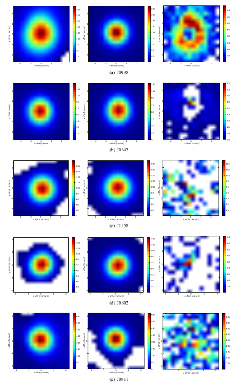
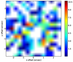
In this paper we analyze the optical spectra of eight galaxies, one is classified as composite HII/S2, 3 sources are classified as S1 (BLS1 & NLS1), and 4 sources are classified as QSOs. Further information about the analyzed objects is presented in Tab. LABEL:all_sources1. In Figs. 2 and 9, we show images of the sources and a nearby reference star extracted from the same image frame.

3.3 Data reduction, wavelength calibration, and flux calibration

Here we describe the data reduction of our spectroscopic observations, wavelength calibration, flux calibration, and the complementary data from public archives that has been used in our analysis.

For reducing the data of the sources listed in Tab. LABEL:all_sources1, we used the python software modsCCDRed, which is provided by the instrument team. This software package gives us the possibility to create bias correction, flat fielding, normalization, and other standard steps of data reduction.

First we create normalized spectral flat field frames for each channel (blue and red) through the following steps:

•

bias correction of the flat fields images;
•

median combination of the bias-corrected flats;
•

interpolation of the bad columns using the bad pixel lists for the detector;
•

elimination of the (wavelength dependant) color term to produce a normalized “pixel flat”.

More information on producing the normalized calibration frames can be obtained from the instrument manual ²²2http://www.astronomy.ohio-state.edu/MODS/Manuals/MODSCCDRed.pdf. After generating the flat, all bias-corrected science data were flat fielded. The science frames were then wavelength-calibrated using a wavelength-calibration map generated from lamp (argon, neon, xenon and krypton) data, as provided by the instrument. In this step, we used the reduction package Iraf to identify the lamp lines and then transformed the science frames accordingly. Furthermore, we tested the wavelength-calibration by using an OH-sky line atlas (Osterbrock et al., 1996; Osterbrock, Fulbright & Bida, 1997) and found that both calibration methods (skylines and lamp) are in good agreement with an uncertainty $\leqslant 3\AA$ .

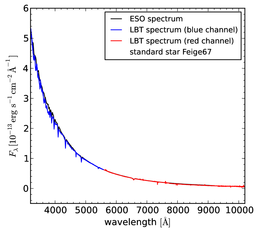
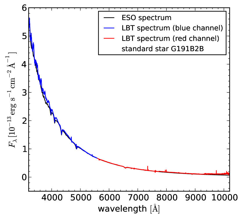
For the next step, we flux-calibrated the one-dimensional spectra making use of two standard stars: G191B2B and Feige67 for which data was taken under 1.3” seeing conditions. Both standard stars result in a consistent and independent calibration. For the final data product we used both stars for calibration. We used reduction routines on two different software platforms: IDL and IRAF. We extract the one-dimensional spectra from the two-dimensional science frames of the two calibration star using routines in the Iraf package. For test purposes we calibrated the two stars with each other and compared the results with published data. We also downloaded spectra of these two standard stars from the European Southern Observatory ³³3http://www.eso.org/sci/observing/tools/standards/spectra/ and compared them with our results (see Fig. 1). Calibrating the science objects with the two reference stars independently resulted in spectra that agreed very well with each other within an average uncertainty of 2% and 3% in the blue and red channel, respectively. We performed that calibration for each source for the red and blue channel and combine these spectra to a single spectrum per source using Iraf. In this process, we found that there are no significant continuum offsets in the overlap area between the red and blue side. While this confirms the consistency of our calibration, the uncertainties in comparing data between different telescopes and instruments is more of the order a few percent, (see e.g., Peterson et al., 2002) i.e. of the same order as reached for the SDSS data releases.

Refer to caption — Figure 1: The standard stars Feige67 and G191B2B.

In order to ensure a sufficient inter-calibration accuracy between telescopes and instruments we applied a correction for slit losses. We observed our target sources (including the two calibrated stars; see above) in typically 1.2 to 1.4 arcsec seeing through a 0.8 arcsec slit. For the two extreme cases we applied a seeing correction based on Fig. 10. For J0153 taken in 1.90” seeing we scaled the LBT fluxes up by a factor of 1.35. For J1203 taken in 0.82” seeing we scaled the LBT fluxes down by a factor of 0.70 SDSS.

In order to correct for a time variable slit loss contribution we proceeded in the following way: For each target we have 2 to 5 exposures such that we have a good statistical estimate on the flux loss due to the combination of variable seeing and misplacement of the slit. In Fig. 10 we show a number histogram of the intensity drop measured in the [OIII] $\lambda$ 5007, [OII] $\lambda$ 3727, H $\beta$ or H $\alpha$ line in the corresponding red and blue channel for the fainter exposures with respect to the brightest once. To first order we correct for this effect by adjusting all exposures to the flux level of the brightest exposure per source. Under the assumption that for the brightest exposure the slit was always centered on the source no additional correction for slit losses is necessary (i.e. a factor of unity; case $\alpha$ in Fig. 10). However, if we assume that no significant systematical misplacements happened and that the statistics for slit losses for the brightest exposures is similar to the statistics of the fainter exposures then an unfavorable and unlikely case will be that all brightest exposures were taken under conditions of a mean slit loss (case $\beta$ in Fig. 10). For a final second order correction for slit losses we assumed a case between case $\alpha$ and case $\beta$ and chose the mean between unity and the factor for mean losses of 1.17 $\pm$ 0.10, i.e. a second order correction factor of 1.08, after having applied the first order correction. Judging from Fig. 10 the uncertainty on this correction for the time variable slit losses is probably of the order of 5% for the 1.2” to 1.4” seeing cases. For J0153 with 1.9” this correction is probably overestimated by $<$ 5% For J1203 with 0.82” seeing our correction may be underestimated by 5-10% especially if one takes into account that for a better seeing slit positioning can also be done more reliably. Given the seeing and aperture combinations for the Beijing and Hiltner telescope measurements (see section 5.7 and 5.6) as well as the high SDSS calibration quality (see section 3.2) no seeing/slit loss corrections were applied to these data.

As we flux calibrate our observed spectra with the flux calibration stars following the procedure presented above and show that the galaxies are all very compact (see section 3.2 and Fig.1 and A.2 and and section 5.1 for the marginally extended source J0938) we assume the inter-calibration uncertainties to be less than 10%.

3.4 Magnitude measurements

In the SDSS survey magnitudes are derived using different methods (Model, Cmodel, Petrosian, and PSF). For our work we used magnitudes derived via the PSF method in which a Gaussian model of the PSF is fitted to the object (dominated by a compact PSF like source). The method also accounts for the variation of the PSF across the field and was hence considered as most suitable for our study.

We compared the flux density value of the photometric observations⁴⁴4We use the Gemini flux density/magnitude converter (http://www.gemini.edu/?q=node/11119) to convert the magnitudes derived from the photometric images in the $u$ , $g$ , $r$ , $i$ , and $z$ -bands into physical units (flux density $\mathrm{{F}_{\lambda}}$ in erg s^-1 cm^-2 Å^-1). with those obtained from spectroscopic observation for each source. In this way we can get an estimate on the degree of variability that is present in the nuclei of these objects.

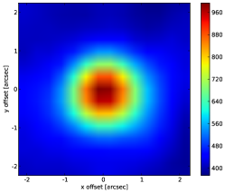
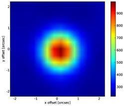
In our LBT observations we used a long slit with aperture of 0 $\aas@@fstack{\prime\prime}$ 8, while for the SDSS observations a spectroscopic fiber with radius $3\arcsec$ was used. To demonstrate that aperture effects between slit and fiber measurements are negligible, we show SDSS $z$ -band images of the galaxies together with images of nearby stars from the same frame (Figs. 2 and 9). We scale the stars to the flux level of the galaxy and subtract the frames from each other. In all eight cases, no emission is left. This shows that the sources are all dominated by emission from an unresolved combination of a stellar bulge and an AGN.

Table 1: Coordinates, redshifts, classification and observing parameters for all sources.

name	RA	Dec.	Redshift (z)	Classi.	Obs. date 1		Obs. date 2	Photo.	$D_{\mathrm{L}}$	Ref.
								obs. date
	(hh mm ss)	( $\degr$ $\arcmin$ $\arcsec$ )			Telesc.	Da.(M Y)	Da.(M Y)	Da.(M Y)	Mpc
SDSS J120300.19+162443.8	12 03 00.1	16 24 43.8	$0.16552\pm 0.00001$	NLS1	SDSS	04 2007	02 2012	06 2005	794.5	1
SDSS J093801.63+135317.0	09 38 01.6	13 53 17.0	$0.10056\pm 0.00001$	HII/S2	SDSS	12 2006	02 2012	01 2006	463.2	2
SDSS J034740.18+010514.0	03 47 40.1	01 05 14.0	$0.03149\pm 0.00003$	NLS1	OHP^a	09 2003	02 2012	11 2001	138.1	3,4
SDSS J115816.72+132624.1	11 58 16.7	13 26 24.1	$0.43966\pm 0.00035$	QSO	SDSS	05 2004	01 2012	03 2003	2429.5	5,6
SDSS J080248.18+551328.9	08 02 48.1	55 13 28.8	$0.66406\pm 0.00035$	QSO	SDSS	01 2005	01 2012	11 2003	3993.9	5,7
SDSS J091146.06+403501.0	09 11 46.0	40 35 01.0	$0.44121\pm 0.00099$	QSO	SDSS	01 2003	02 2012	12 2001	2439.7	5,6
2MASX J03540948+0249307^∗	03 54 09.4	02 49 30.7	$0.03600\pm 0.00008$	BLS1	Hiltner^b	10 2004	02 2012	—	158.4	3,8
GALEXASC J015328.23+260938.5^∗	01 53 28.2	26 09 39.1	$0.32640\pm 0.00127$	QSO	Beijing^c	02 2002	01 2012	—	1711.9	9,10

References for redshifts and positions: (1) Adelman-McCarthy & et al. (2011); (2) Sánchez Almeida et al. (2011); (3) Véron-Cetty & Véron (2006); (4) Hewitt & Burbidge (1991); (5) Hewett & Wild (2010); (6) Zhang et al. (2010); (7) Gibson et al. (2009); (8) Chanan, Downes & Margon (1981); (9) Darling & Giovanelli (2002); (10) Zhou et al. (2002).
Notes: The 3 QSOs (J1158, J0911, J0802) contained in the SDSS catalogue have been classified as low-ionization broad absorption-line (loBAL) due to a prominent [Mg ii] absorption in their spectra. The second spectroscopy observation have always taken by LBT. The photometric observations were always taken by SDSS. For the final two sources in the table no SDSS photometric observations are available.
^∗ Not covered by SDSS survey
^a Telescope of Observatoire de Haute-Provence (OHP)
^b Hiltner Telescope
^c Beijing Observatory

Table 2: Comparison of seeing conditions for the sources for which we analyzed the spectra.

Sources	LBT seeing	Comparing Spectro.		SDSS photometric
		Inst.	seeing	Median Seeing (r-band)
	″		″	″
J1203	0.82	SDSS	1.48	1.4
J0938	1.30	SDSS	1.69	1.4
J0347	1.40	OHP	2.5	1.4
J1158	1.40	SDSS	1.22	1.4
J0802	1.20	SDSS	1.49	1.4
J0911	1.20	SDSS	1.23	1.4
J0354	1.20	Hiltner	2.5	–
J0153	1.90	Beijing	2.5	–

Table 3: The observed continuum flux density variability between LBT and SDSS/OHP of J0938, J1203, J1158, J0911, J0802, and J0347 from the photometry and spectroscopy aspect. ^(a)For J0347 first epoch spectroscopy obtained by OHP.

Sources	Filt.	Wa.	photometry	Emission line	spectroscopy	spectroscopy
			SDSS	contribution in	SDSS^(a)	LBT
		Å	[ $10^{-16}\,\mathrm{erg}$	spectral filters	[ $10^{-16}\,\mathrm{erg}$	[ $10^{-16}\,\mathrm{erg}$
			$\mathrm{s}^{-1}\ \mathrm{cm}^{-2}\AA^{-1}$ ]	in % of continuum	$\mathrm{s}^{-1}\ \mathrm{cm}^{-2}\AA^{-1}$ ]	$\mathrm{s}^{-1}\ \mathrm{cm}^{-2}\AA^{-1}$ ]
J1203	(u)	3543	$1.26\pm 0.03$		—	$2.04\pm 0.99$
	(g)	4770	$1.06\pm 0.02$	9	$1.20\pm 0.19$	$1.54\pm 0.38$
	(r)	6231	$1.53\pm 0.01$	25	$1.02\pm 0.31$	$0.87\pm 0.13$
	(i)	7550	$1.09\pm 0.01$	33	$0.81\pm 0.21$	$0.61\pm 0.14$
	(z)	9134	$0.53\pm 0.03$		$0.65\pm 0.32$	$0.49\pm 0.13$
J0938	(u)	3543	$1.60\pm 0.03$		—	$1.87\pm 0.31$
	(g)	4600	$2.39\pm 0.02$	2	$3.41\pm 0.19$	$2.66\pm 0.27$
	(r)	6231	$2.01\pm 0.02$		$3.30\pm 0.15$	$2.48\pm 0.31$
	(i)	7625	$1.67\pm 0.02$	7	$3.05\pm 0.17$	$2.36\pm 0.41$
	(z)	9134	$1.50\pm 0.02$		$2.79\pm 0.27$	$2.12\pm 0.45$
J0347^(a)	(u)	3543	$68.81\pm 0.01$		—	$52.79\pm 0.09$
	(g)	4770	$53.90\pm 0.02$	6	$44.60\pm 0.21$	$60.38\pm 0.02$
	(r)	6231	$44.92\pm 0.01$	36	$31.12\pm 0.15$	$39.23\pm 0.01$
	(i)	7625	$40.91\pm 0.02$		$27.71\pm 0.11$	$33.81\pm 0.02$
	(z)	9134	$26.93\pm 0.01$		—	$26.39\pm 0.04$
J1158	(u)	3543	$5.98\pm 0.04$		—	$5.12\pm 0.63$
	(g)	4770	$4.29\pm 0.02$	5	$4.62\pm 0.23$	$3.91\pm 0.33$
	(r)	6400	$2.87\pm 0.02$		$2.81\pm 0.14$	$3.31\pm 0.16$
	(i)	7700	$2.21\pm 0.02$	6	$2.15\pm 0.16$	$2.65\pm 0.03$
	(z)	9134	$1.77\pm 0.03$		$1.48\pm 0.48$	$1.87\pm 0.07$
J0802	(u)	3543	$0.41\pm 0.06$		—	$0.88\pm 0.49$
	(g)	4770	$0.97\pm 0.01$		$1.02\pm 0.12$	$1.37\pm 0.11$
	(r)	6231	$1.17\pm 0.01$	2	$1.14\pm 0.11$	$1.49\pm 0.06$
	(i)	7625	$1.24\pm 0.02$	3	$1.16\pm 0.20$	$1.71\pm 0.10$
	(z)	9134	$1.04\pm 0.02$		$0.97\pm 0.25$	$1.23\pm 0.29$
J0911	(u)	3543	$0.89\pm 0.04$		—	$0.61\pm 0.27$
	(g)	4770	$0.86\pm 0.02$	5	$0.67\pm 0.04$	$0.92\pm 0.22$
	(r)	6200	$0.85\pm 0.01$		$0.90\pm 0.04$	$1.10\pm 0.15$
	(i)	7700	$0.68\pm 0.02$	7	$0.72\pm 0.03$	$0.96\pm 0.07$
	(z)	9134	$0.54\pm 0.03$		$0.56\pm 0.10$	$0.76\pm 0.19$

Table 4: Comparison of the apparent sizes of the sources and reference stars in the field.

source	Star		Star			Galaxy
	RA	Dec.	FWHM1	FWHM2	Angle	FWHM1	FWHM2	Angle
	(hh mm ss)	( $\degr$ $\arcmin$ $\arcsec$ )	″	″	″	″	″	″
J1203	12 02 59.4	16 24 20.5	$0.95\pm 0.03$	$1.03\pm 0.03$	$1.24\pm 0.56$	$1.26\pm 0.15$	$1.09\pm 0.09$	$10.97\pm 0.29$
J0938	09 38 22.3	13 49 54.4	$1.15\pm 0.01$	$1.04\pm 0.01$	$0.97\pm 0.13$	$1.31\pm 0.07$	$1.11\pm 0.08$	$1.88\pm 0.48$
J0347	03 47 35.8	01 04 08.6	$0.99\pm 0.01$	$1.31\pm 0.01$	$1.81\pm 0.15$	$1.09\pm 0.01$	$1.35\pm 0.01$	$0.87\pm 0.16$
J1158	11 58 14.2	13 25 57.0	$1.43\pm 0.02$	$3.76\pm 1.48$	$0.92\pm 0.30$	$1.44\pm 0.04$	$1.49\pm 0.04$	$0.64\pm 0.48$
J0802	08 01 38.2	55 11 44.2	$0.57\pm 0.01$	$0.60\pm 0.01$	$0.78\pm 0.17$	$0.67\pm 0.04$	$0.52\pm 0.03$	$49.44\pm 0.46$
J0911	09 11 47.7	40 34 38.9	$0.75\pm 0.04$	$0.81\pm 0.04$	$3.22\pm 0.82$	$0.87\pm 0.06$	$0.91\pm 0.06$	$0.79\pm 0.90$

Notes: For each galaxy, we give the coordinates of the star that we subtracted from the galaxy image as well as results of a Gaussian fit to galaxy and star. We used an elliptically shaped Gaussian function.

Furthermore, we fitted Gaussian functions to the images of the galaxies and the stars. The results are listed in Tab. LABEL:all_sources2, supporting the finding that the galaxy emission is dominated by the unresolved point source. In Tab. LABEL:seeing we list the seeing values for the different exposures.

4 Analysis

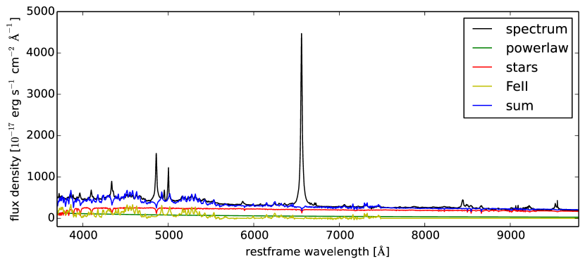
We developed a Python routine to manually fit the stellar continuum, the power-law contribution from the AGN, as well as the Fe ii emission and subtract all of them. In the residual spectrum we can then fit the non-Fe ii emission lines. In following we explain each step:

4.1 Stellar continuum subtraction

To obtain an accurate measurement of the nuclear emission line fluxes and the equivalent widths, we have to subtract the stellar component of the host or its bulge component. To remove the stellar component we fitted a stellar population synthesis model to the entire spectrum. The templates used are given by a sample spectrum built by a population synthesis routine in Bruzual & Charlot (2003). The template for the young stellar population spectrum is taken 290 Myr after a starburst with steady star formation rate over 0.1 Gyr and solar metalicity. For the intermediate-age population we used template of a 1.4 Gyr old simple stellar population with solar metalicity.

Table 5: Continuum fits.

name	instrument	$A_{V}$ (stars)	stars	powerlaw	Fe ii
J1203	LBT	0	60%	40%	0%
	SDSS	0	60%	40%	0%
J0938	LBT	1.5	90%	10%	0%
	SDSS	1.5	80%	20%	0%
J0347	LBT	1.2	57%	20%	23%
	OHP	0.8	72%	13%	15%
J1158	LBT	0	0%	85%	15%
	SDSS	0	0%	85%	15%
J0802	LBT	0	50%	30%	20%
	SDSS	0	52%	33%	15%
J0911	LBT	0	50%	40%	10%
	SDSS	0	45%	45%	10%
J0354	LBT	1.8	60%	30%	10%
J0153	LBT	0	62%	23%	15%

Notes: For each observation we give the flux contributions of the stellar component, the AGN/powerlaw component, and the Fe ii template, as well as the extinction $A_{V}$ of the stellar component in the wavelength interval $5100\,\mathrm{\AA}$ to $5600\,\mathrm{\AA}$ (restframe wavelength).

In Tab. LABEL:tab:contfit we show the flux contributions of the stellar component, the AGN/powerlaw component, and the Fe ii template, as well as the extinction $A_{V}$ of the stellar component. We measured the fraction of each component compared to the total flux in the (restframe) wavelength interval $5100\,\mathrm{\AA}$ to $5600\,\mathrm{\AA}$ . The main purpose of the subtraction was to remove the Fe ii emission lines from the spectrum, particularly those blended with other emission lines. Since in most galaxies there are no obvious stellar features, it is difficult to distinguish between different stellar populations. Therefore, we sum up the contributions of the intermediate-age and the young stellar population. Also the fit of the extinction $A_{V}$ is not reliable, but was only chosen to fit the continuum slope as accurate as possible. The data for the line variability as discussed in Sect. 6 includes all corrections derived from the fitting described here.

4.2 Fe ii subtraction

The optical emission-lines of Fe ii are typical features of Seyfert 1 galaxies and quasars. There is huge variety in the strength of these lines, from very clearly shaped and detectable lines in some AGN spectra, all the way to very weak and imperceptible lines in other sources. Boroson & Green (1992) (in the following BG92) reported a strong inverse correlation between the strength of Fe ii emission-lines and the width of the broad $\mathrm{H\beta}$ line as well as the strength of the [O iii] line. This result was confirmed by other groups (e.g., Corbin, 1997; Zhou et al., 2006; Kovačević, Popović & Dimitrijević, 2010; Dong et al., 2011). For our work we used the Fe ii template from BG92, fitted and scaled to our galaxy spectra as shown in Fig. 3. Tab. LABEL:tab:contfit shows that the contribution of Fe ii in the given wavelength range is up to 23% and a proper subtraction of Fe ii is required, so the fitted spectra were then subtracted from our spectra. Finally, we obtained a spectrum corrected for both the host continuum (as mentioned in Sect. 4.1) and Fe ii.

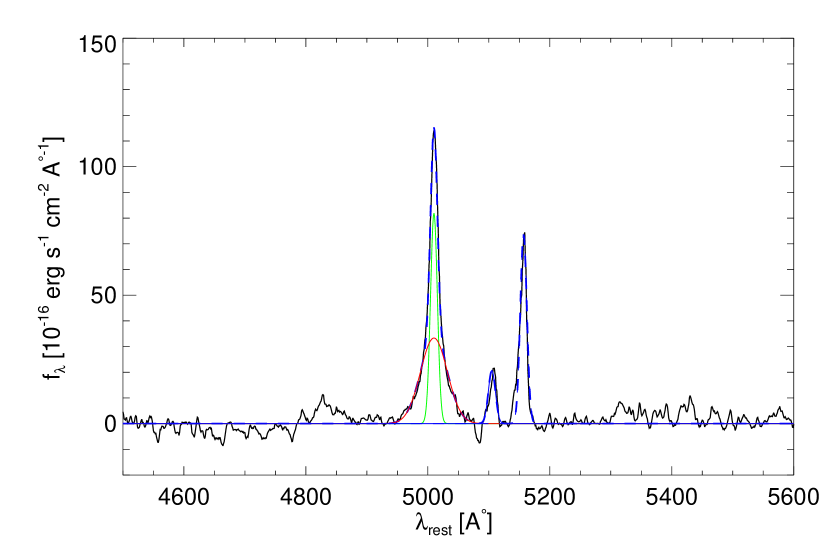
4.3 Emission-line fitting

To accurately measure the fluxes of emission lines, we used mpfitexpr (Markwardt, 2009). We fitted several Gaussians or a single Gaussian to the line profile, to fit narrow or broad components depending on the details of their shape or the presence of neighboring features. For example, to fit the H $\alpha$ +[N ii] complex, we used four Gaussians components, where the flux ratio of the [N ii] $\lambda$ 6583 Å, 6548Å doublet is fixed to the theoretical value of 2.96. In addition, their widths are supposed to be identical. Likewise, for the complexes of H $\beta$ +[O iii] $\lambda$ 5007 Å, we fitted three Gaussians components as shown in Fig. 4, and two Gaussian components if the H $\beta$ line is narrow. Additionally, for some broad lines we fitted a Lorentzian profile if the width of the lines cannot be represented by Gaussian line profiles. The results of the line fitting are listed in Tab. 9.

5 Results

Redshifts and luminosity distances $D_{\mathrm{L}}$ (Hogg, 1999) are listed in Tab. LABEL:all_sources1. The luminosity distances $D_{\mathrm{L}}$ were calculated using the redshift of the source combined with the cosmology constants assuming a Hubble constant $H_{0}=70\ \mathrm{km}\ \mathrm{s}^{-1}\ \mathrm{Mpc}^{-1}$ , and a standard cosmology with parameters $\Omega_{\mathrm{m}}=0.3$ , and $\Omega_{\Lambda}=0.7$ (Spergel et al., 2003, which we use throughout the paper).
The observed continuum flux density variability of the sources derived from LBT and SDSS data is summarized in Tab. LABEL:fig:variab.

The main body of comparative variability studies of extragalactic nuclei is carried out without a detailed differentiation of contributions of different spectral components to the overall emission. For the brighter QSOs this can be justified since the host contribution is small. Such a spectral analysis requires a very high signal to noise in order to determine the exact nature of the stellar host contribution which in return is dependant on the modeling details of the dominant contributing stellar populations. Given the inter-calibration quality for the newly presented 8 sources such a analysis shows that around 5500 Å (restframe wavelength) the stellar contribution to the integrated flux for the S2/NLS1 source is $\geq$ 50% and for the QSOs it is $\leq$ 50%. However, the quality of the data does not allow to study the variability of the power spectrum component alone, since the details of the stellar population analysis required a much higher data quality. Hence, the difference in the continuum variability properties between S2/NLS1 and QSO/BLS1 presented in this paper is influenced by the presence of a stronger stellar contribution for the S2/NLS1. Details are given in column 5 of Tab. LABEL:fig:variab. If no value is given in column 5 then the contamination is below 5%.

The variability of a larger sample (see section 6.1) is discussed with continuum and line variability extracted from spectra. In order to avoid contamination from the host and the Fe-lines, the line variability is measured from spectra corrected for these contributions (see subsections above). However, in order to be able to enlarge the sample with data from the literature, the continuum variability measurements do contain the stellar flux contribution. The effects of this are discussed in section 6.3.

The line fitting results are listed in Tab. 9. We plot all our spectra in the rest wavelength as shown in Fig. (5, 11, 17, etc.). We did that by applying $\lambda_{rest}=\lambda_{obs}/{1+\mathrm{z}}$ . Another correction was applied to the flux density (cosmological dilution), changing this value to the rest system via

F_{\lambda}\ rest=F_{\lambda}\ obs.\times(1+\mathrm{z})^{3}~{}~{}~{}.

(1)

All continuum flux densities and luminosities listed in the tables are derived as observed quantities (i.e. without corrections). The listed line fluxes and luminosities have been corrected for FeII and stellar continuum as described above.

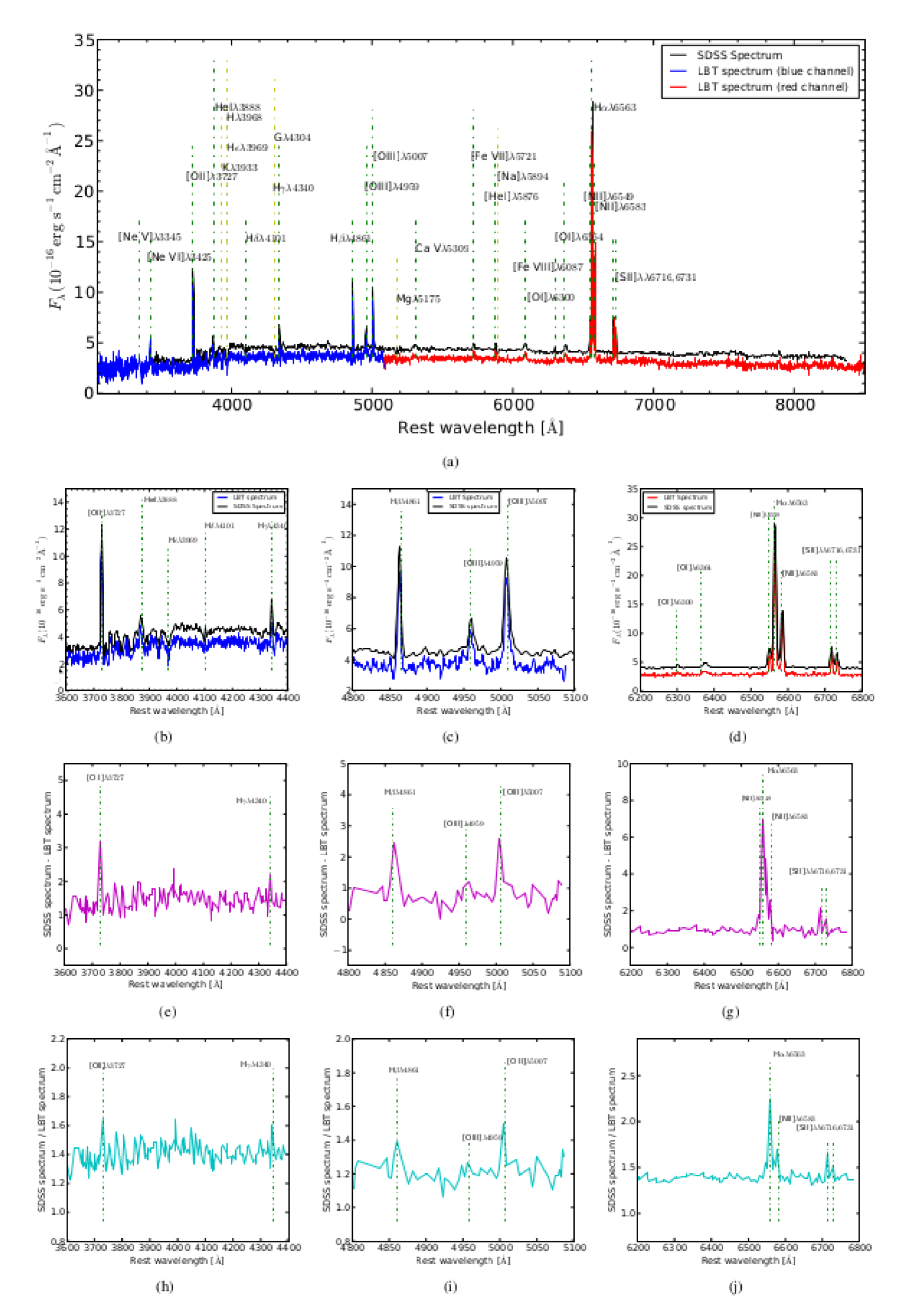
5.1 SDSS J093801.63+135317.0

SDSS J093801.63+135317.0 (hereafter J0938) is discussed in the discovery of a population of normal field galaxies that have luminous and strong FHIL (forbidden high by ionized lines) and HeII $\lambda$ 4686 emission (Stepanian & Afanas’ev, 2011). The authors used the ’Bolshoi Teleskop Alt-azimutalnyi BTA-6’ 6-m diameter telescope in Russia and obtained spectra with 0.86Å/px resolution. Stepanian & Afanas’ev (2011) report, in their Table 2, the value of FWHM and flux for emission lines in the optical spectrum of J0938 taken with two instruments with the same spectral resolution of $R\sim 2000$ at two different epochs. The first is from the SDSS telescope on 18.12.2006 and the second is from the BTA-6 on 16.04.2010.

Yang et al. (2013) present results of seven rare extreme coronal line emitting galaxies, and J0938 is also among these sources. These objects are reported by Wang et al. (2012), and four of these galaxies (J0938 and three others) have a large variability in coronal line flux, making them good candidates for tidal disruption events (TDEs). They detected a broad He II $\lambda$ 4686 emission line in the spectrum of J0938. Yang et al. (2013) find broad coronal and high-ionization lines that are superimposed on narrow low-ionization lines. They interpret this finding as indication that J0938 is a composite of a S2 nucleus and a star formation region. In the SIMBAD catalogue the object is listed as an H ii galaxy. However, according to the [O i] $\lambda$ 6300/H $\alpha$ versus [O iii] $\lambda$ 5007/H $\beta$ diagnostic diagram in Wang et al. (2012) and Yang et al. (2013) it’s appearance to be that the source J0938 is located in the region between H ii and S2 galaxies (here we adopt an HII/S2 composite nucleus classification) and belongs to a sample of sources with spectra that are dominated by the interaction of a super massive black hole with the nuclear environment (Stepanian & Afanas’ev, 2011; Wang et al., 2012; Yang et al., 2013).

The variability data for this source are consistent with the uncertain classification of the source as HII/S2 and support the presence of a variable nucleus. In Tab. LABEL:fig:variab we list the flux density measurements of J0938 for three epochs at different wavelengths as obtained through our LBT observations and via the spectroscopy and photometry results listed by SDSS. We note that flux values of the continuum of LBT spectroscopy are in good agreement with photometric data of SDSS at the same wavelengths, while both are different to what can be derived from SDSS spectroscopy. We notice that their are of order 30% variations in line and continuum flux between the different epochs we use for our investigation.

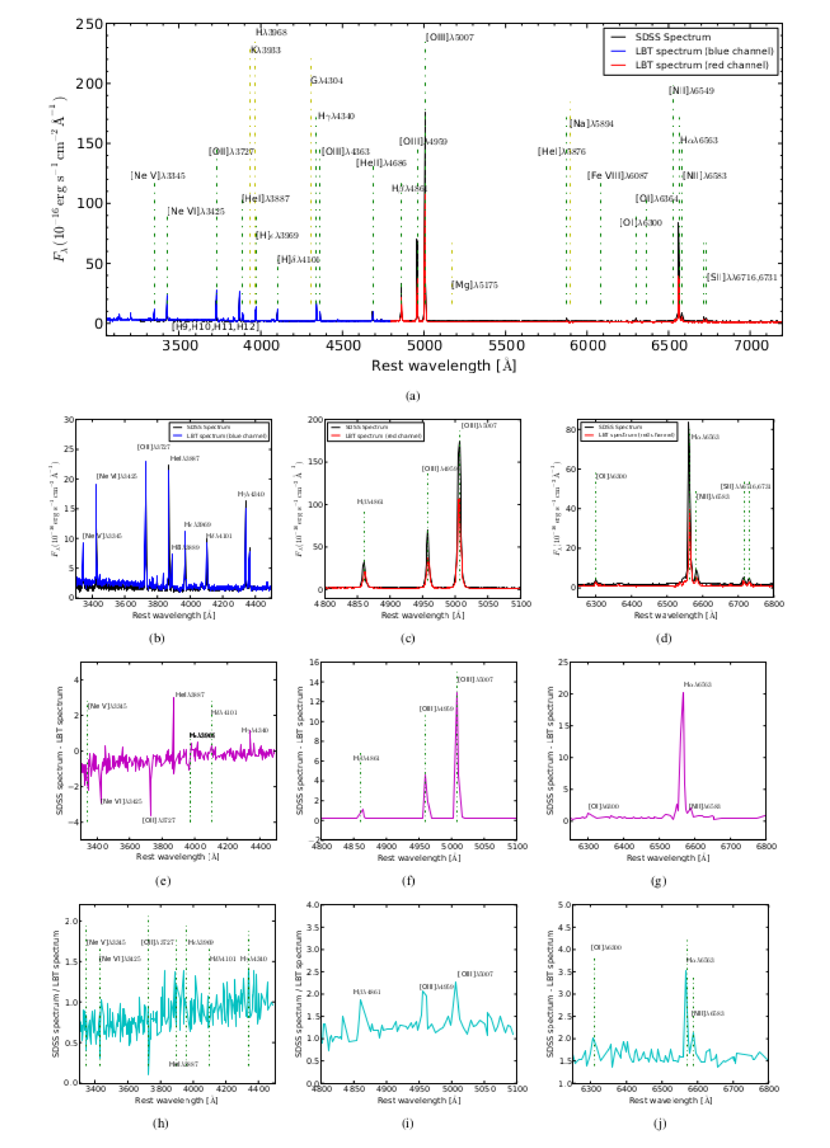
As we show in Fig. 9, and as is evident from the data in Tab. LABEL:all_sources2, the host of the source is extended. Comparison with stars in the field show that about 50% to 60% of the continuum flux in the LBT 0.8” slit is due to the unresolved nuclear component. The rest can be attributed to the a contribution of the extended host. Hence the estimated continuum variability is probably only an upper limit. However, for completeness we leave the variability estimates in Fig. 6 as upper limits. The median and median deviation derived from this plot are not effected by this. In Fig. 5 we over-plot the two optical spectra (LBT and SDSS) of J0938. The LBT spectrum was observed in 2012, and the SDSS spectrum was taken in 2006. Therefore, we can discuss the variability on a time scale of 6 years. We found that, for this object, there are two types of variability: first, there is variability in the continuum level between the two spectra, where the continuum level of the SDSS spectrum is higher by a factor of $\sim$ 1.3 than that of the LBT spectrum. This can be seen in Fig. 5 (a,b,c,and d) where we plot different sections of the J0938 spectrum. The second type of the variability is in the emission lines. To show this we subtract the two spectra from each other and plot the difference (Fig. 5 e, f, and g). Additionally, we show the variability of these lines by displaying the ratio of the two spectra (Fig. 5 h,i, and j). We found that the emissions lines that varied most in the spectrum of J0938 are [O ii], $\mathrm{H\beta}$ , [O iii] $\lambda$ 5007, and $\mathrm{H\alpha}$ . The $\mathrm{H\alpha}$ and [O iii] lines show a variation of the order 1.25. The measured line fluxes are listed in Tab. 9.

5.2 SDSS J120300.19+162443.8

SDSS J120300.19+162443.8 (henceforth J1203) has been mentioned in Shirazi & Brinchmann (2012) among 2865 galaxies to have a strong nebular He II $\lambda$ 4686 emission. A strong He II $\lambda$ 4686 line indicates that the nuclear radiation field of these objects is dominated by highly ionizing radiation. The ionization potential of $\mathrm{He^{+}}$ is 54.4 eV corresponding to a UV photon wavelength of $\lambda\approx 228\AA$ .

In Tab. LABEL:fig:variab we list the flux densities $\mathrm{{f}_{\lambda}}$ of J1203 at different wavelengths obtained from our LBT data and spectroscopy and photometry data as listed by SDSS. We note that the flux values of the continuum at different wavelength indicate variability. Moreover, the power law index of the continuum feature of both observations SDSS (photometric & spectroscopy) and LBT (spectroscopy) has also varied as we show in the optical spectrum of J1203 in Fig. 11.

The optical emission line spectrum of J1203 is dominated by a NLR (see Fig. 11). In Tab. 9 we see that all the emission lines are narrow with FWHM values of $\leqslant 8.3\AA$ (where $8.3\AA\ \approx 500$ $\mathrm{km}\ \mathrm{s}^{-1}$ ). J1203 has very low count rates at the continuum level. The H $\alpha$ complex gives indications of a possible faint broad component. Barth et al. (2014) find that all S2 candidates in their sample for which high spectral resolution deep exposures had been taken showed some broad line emission that was not visible in previous spectra. A comparison between the [OIII] $\lambda$ 5007 and H $\beta$ line shows a very similar line profile, within the uncertainties, hence we classify J1203 as a S2 galaxy.

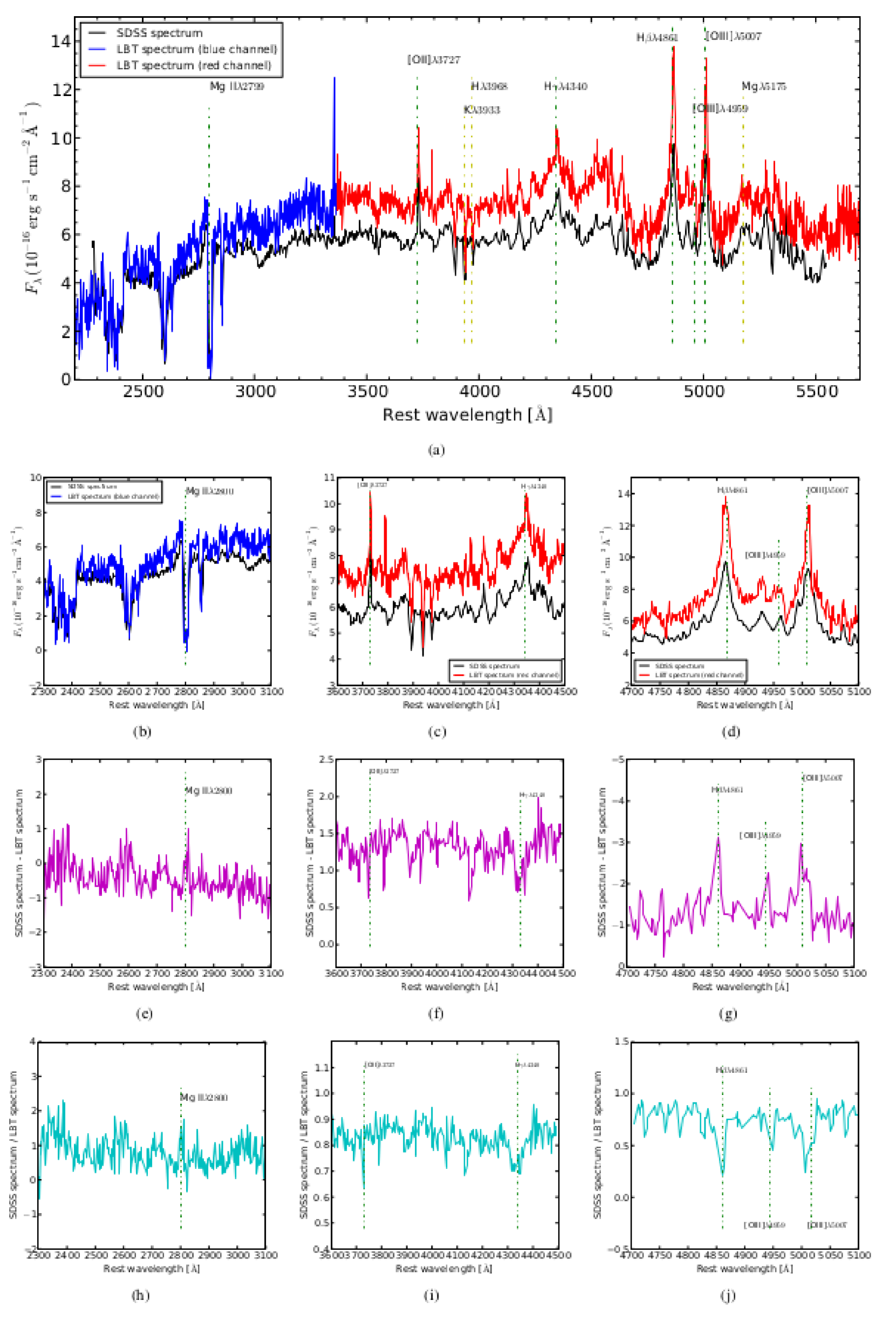
The over-plot of the two optical spectra (LBT and SDSS) for J1203 is presented in Fig. 11. The SDSS spectrum was observed in 2007, while the LBT spectrum was observed in 2012. Hence, for this galaxy we can discuss the variability that happened over 5 years. We find that the continuum variability here is rather limited to the blue channel region from $3300\AA$ to $3700\AA$ where effects of red wing of the ”Big Blue Bump BBB” may well be present (Gaskell, 2008; Starling & Puchnarewicz, 2001), as shown in Fig. 11 (d). The observed continuum of the LBT spectrum in this region is higher than the SDSS spectrum. But for the rest of the spectrum both spectra are at the same level till 6000 Å. The line emission varies by about 40% (see Tab. 9).

5.3 SDSS J115816.72+132624.1

The optical spectrum of SDSS J115816.72+132624.1 (hereafter J1158; observing dates see Tab. LABEL:all_sources1) is strongly dominated by Fe ii lines (as can be seen in Fig. 12 and as reported also in Kovačević, Popović & Dimitrijević, 2010; Dong et al., 2011). Tab. LABEL:fig:variab shows that the flux values of the photometric and spectroscopy observations obtained within the SDSS survey are in good agreement. However, both values show a difference with respect to the flux value extracted from the LBT spectrum, indicating variability. In Wang & Rowan-Robinson (2009) the authors refer to J1158 as a faint source and mention it in the Imperial IRAS-FSC Redshift Catalogue (IIFSCz) among 60303 galaxies. Verifying the consistency of source positions they improved the optical, near-infrared, radio identification. According to Zhang et al. (2010) J1158 is classified as a low-ionization broad absorption-line (loBAL) quasar, with [Mg ii] absorption-lines with a width of $\Delta\upsilon_{c}\geqslant 1600\ \mathrm{km}\ \mathrm{s}^{-1}$ . Additionally, the authors calculate the continuum luminosity at $5100\AA$ ( $\lambda L_{5100}$ ) as $7.7\times 10^{44}\mathrm{erg}\ \mathrm{s}^{-1}$ . From the LBT spectrum we obtain a luminosity at the same wavelength with a flux of $2.81\times 10^{45}\mathrm{erg}\ \mathrm{s}^{-1}$ . The SDSS spectrum results in a value of $2.25\times 10^{45}\mathrm{erg}\ \mathrm{s}^{-1}$ . Consistent with the fluxes listed in Tab. LABEL:fig:variab we can conclude that the continuum luminosity of this source has varied by a factor of 1.2 over the past 8 years.

In Fig. 12 we present the over-plot of the LBT and SDSS spectra for J1158. The LBT data have been obtained in January 2012, and the SDSS survey monitored this source in May 2006. Hence, for this object we are able to study and discuss the spectral variability on a time scale of 6 years. After over-plotting both spectra and measuring the flux densities of the emission lines (Tab. 9) for this galaxy, we found that the variability in the continuum level and the continuum spectral index (hereafter PLI) may well be coupled to each other as the red tail of the BBB may be the dominant contributor to the variability behavior. In addition we find strong variability in emission line intensity.

As shown in Fig. 12 (a,b,c, and d) the continuum level of the LBT spectrum is higher than that in the SDSS spectrum by a factor of about 1.25. This could be linked to power-law variability over the entire optical spectrum as expected from localized temperature fluctuations of a simple inhomogeneous disk (Ruan et al., 2014). We find the PLI for both spectra to vary from -0.21 $\mathrm{erg}\ \mathrm{s}^{-1}\ \mathrm{cm}^{-2}$ / Å for the SDSS spectrum to the PLI of LBT spectrum of -0.01 $\mathrm{erg}\ \mathrm{s}^{-1}\ \mathrm{cm}^{-2}$ / Å. Among them the H $\beta$ $\lambda 4861$ and [O iii] $\lambda 5007$ line show the strongest variation by a factor of about 3. In general, the emission lines in this source are more variable than in other objects of our sample.

5.4 SDSS J091146.06+403501.0

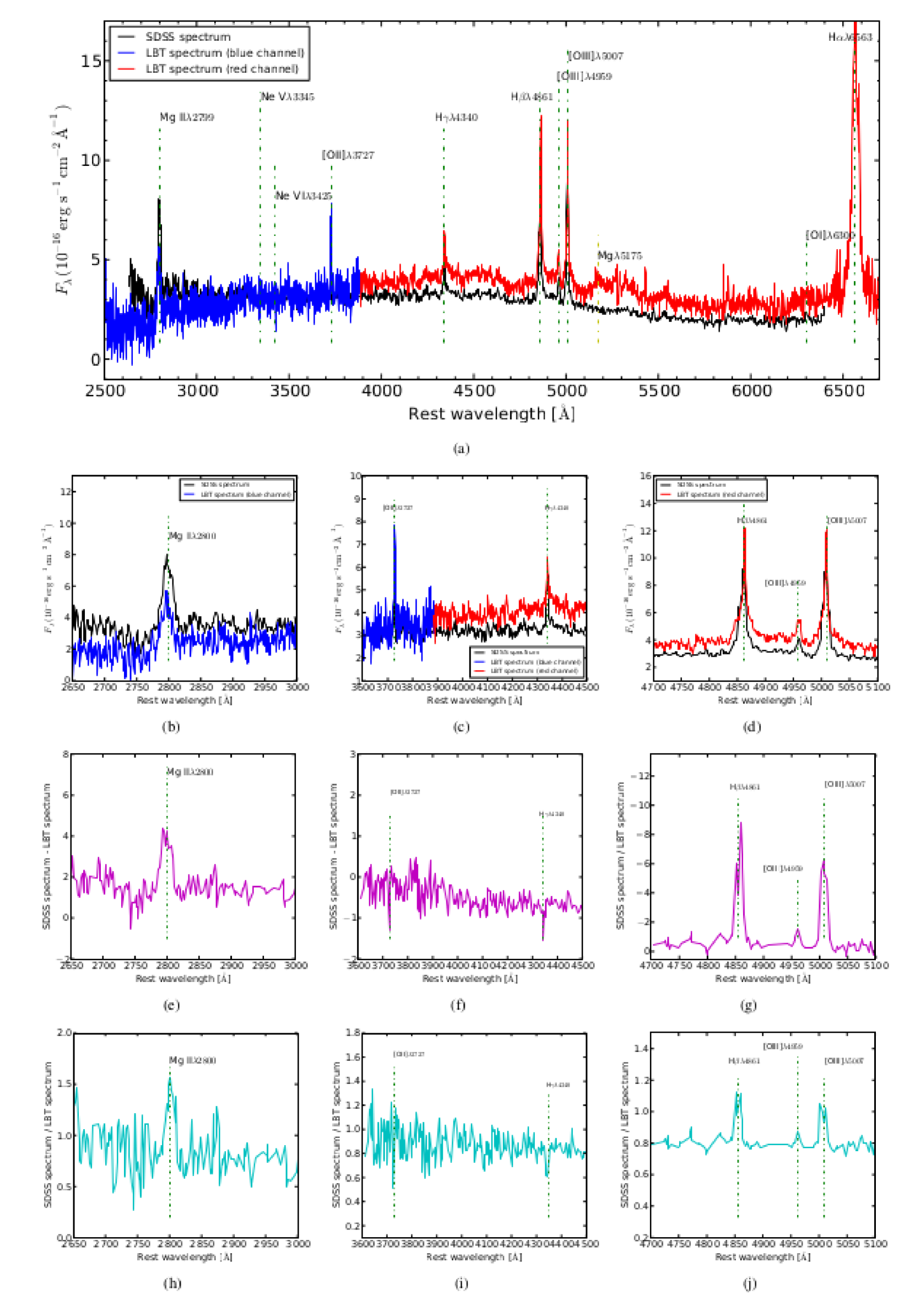
SDSS J091146.06+403501.0 (hereafter J0911) was first reported in McMahon et al. (2002) as a radio source. In the third data release of the SDSS survey (Schneider et al., 2005) it is classified as a quasar. Zhang et al. (2010) classify J0911 as a low-ionization broad absorption-line (loBAL) quasar, with [Mg ii] absorption-line in its spectrum with a line width of $\Delta\upsilon_{c}\geqslant 1600\ \mathrm{km}\ \mathrm{s}^{-1}$ . J0911 exhibits strong Fe ii lines as shown in Fig. 13. Based on the SDSS DR5 data Zhang et al. (2010) calculate the continuum luminosity of J0911 at $5100\AA$ ( $\lambda L_{5100}$ ) to be $2.9\times 10^{44}\mathrm{erg}\ \mathrm{s}^{-1}$ , while at the same wavelength we derive from our LBT spectroscopy data a luminosity value of $3.66\times 10^{44}\mathrm{erg}\ \mathrm{s}^{-1}$ , and for the SDSS spectrum we find $2.84\times 10^{44}\mathrm{erg}\ \mathrm{s}^{-1}$ . These three values, and the measurements in Tab. LABEL:fig:variab, show that there is significant variability in the continuum emission of this source over these two epochs (see Fig. 13). This is in contrast to the strong variability we find for J1158 and supports the consistency of the calibration between the different data sets. As part of the SDSS survey this source has been observed in March 2003, while the LBT spectrum of the source was taken in February 2012. Hence we look at a time span of 9 years for the variability search. The optical spectra of J0911 can be seen in Fig. 13 (a, b, c, and d). As illustrated in this figure, the variability of the source is small compared to other sources in the sample, except for the blue part of the spectrum in Fig. 13 (b), where we see a difference in the continuum slope. This variation in the blue part of the continuum may caused by an accelerating outflow emanating from the black hole in the center of the galaxy, see Shapovalova et al. (2010). In Tab. 9 we list the flux measurements of the emission lines and their FWHM.

5.5 SDSS J080248.18+551328.9

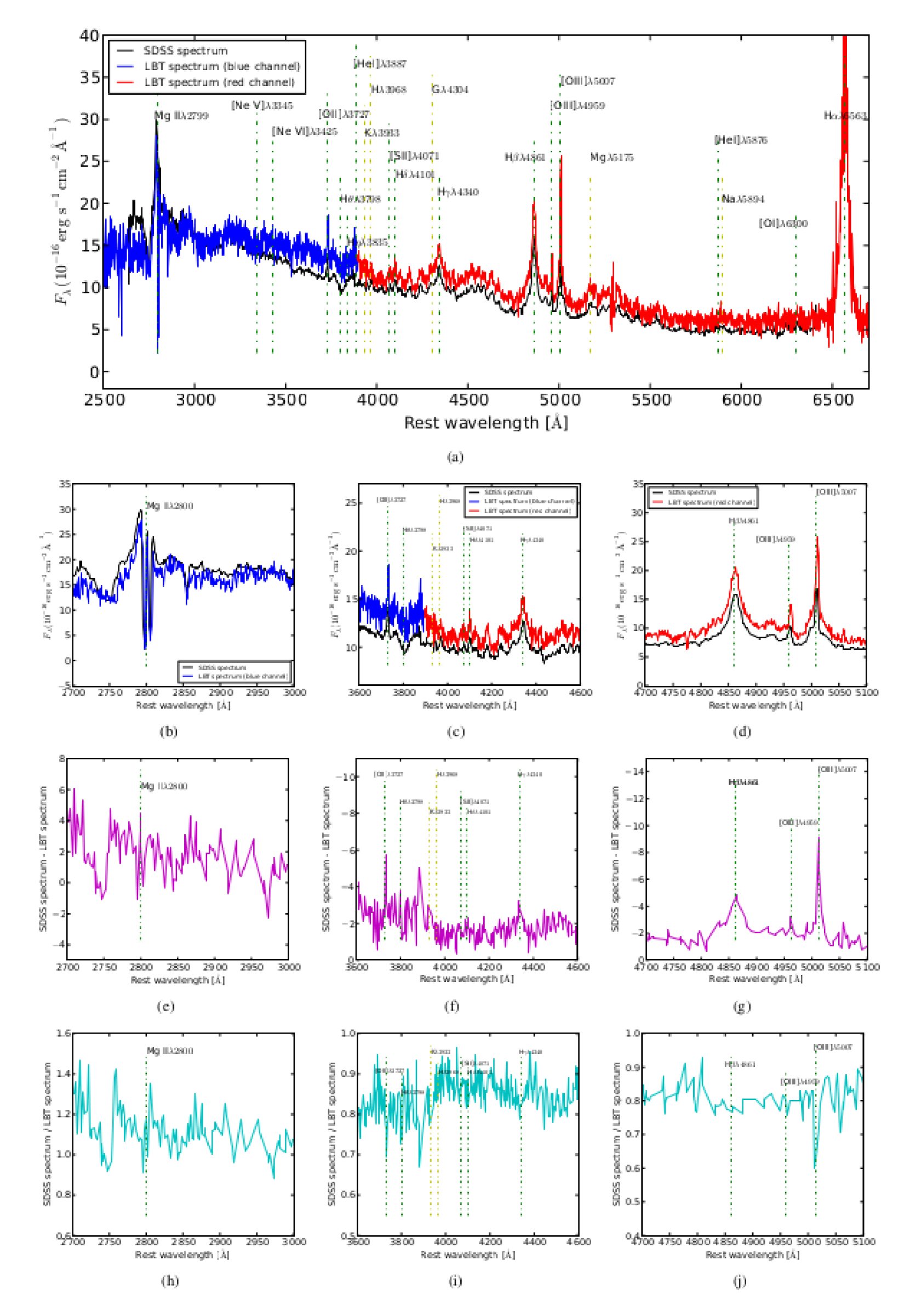
SDSS J080248.19+551328.9 (in the following J0802) was first mentioned in the Fifth Data Release DR5 of the SDSS catalog for quasars (Schneider et al., 2007). The initial redshift determination $\mathrm{z}=0.66287\pm 0.00107$ in DR5 (Schneider et al., 2007), later has been corrected to a value of $\mathrm{z}=0.664065\pm 0.000355$ (Hewett & Wild, 2010). Schneider et al. (2010) and Inada et al. (2012) classified J0802 as a quasar, which is supported by Gibson et al. (2009), Lundgren et al. (2009) and Allen et al. (2011) with reference to a broad absorption line of [Mg ii] $\lambda 2800$ in its spectrum. From the optical spectra it is apparent that J0802 is highly dominated by Fe ii lines (see Fig. 14). We notice that the continuum power law index derived from the LBT and SDSS spectroscopy data as well as the value derived from SDSS photometry are in good agreement (Tab. LABEL:fig:variab). According to these data the continuum spectrum peaks in the i-band. However, comparing the flux densities we find that while values of SDSS photometric and LBT spectroscopy are similar they both are different to what can be derived from SDSS spectroscopy. This indicates that J0802 shows some continuum variability between epochs.

The LBT spectrum was observed in January 2012, while the SDSS spectrum was taken in January 2005, resulting in a time baseline of 7 years for this source. Plotting both spectra (SDSS & LBT) for J0802 in Fig. 14 (a, b, c, and d) we find that there are spectral similarities to the source J0938. Both spectra have the same continuum slope but the continuum level of the LBT spectrum is higher by a factor of 1.3 compared to the SDSS spectrum. The intensity of the emission lines in LBT spectrum are stronger than those obtained from the SDSS spectrum (see Tab. 9). The H $\gamma$ $\lambda$ 4340 line shows the strongest variation with a factor of about 2.

5.6 2MASX J035409.48+024930.7

This source 2MASX J035409.48+024930.7 (hereafter J0354) is one of the two sources that have not been covered by the SDSS survey. J0354 was serendipitously discovered and discussed, together with 18 other objects, in Chanan, Downes & Margon (1981) as an AGN X-ray source. In Bothun et al. (1982) the authors report that the J0354 spectrum ( $\mathrm{M_{V}\sim 18}$ ) allows for either QSO or Seyfert 1 classification. They outline that compared to other samples (e.g., Margon, Chanan & Downes, 1982) the object is amongst the brightest X-ray sources. They also report that this source has a large ratio of X-ray to optical luminosity $\mathrm{L}_{x}/\mathrm{L}_{opt}=2$ which is above the typical ratio of 0.5 found for quasars. Haddad & Vanderriest (1991) state that J0354 is a gas rich galaxy that arose from a two-galaxy interaction, where the larger one is either a quasar or S1 and the second clearly shows signs of tidal distortion. Hutchings, Campbell & Crampton (1982) suggest that the companion is bluer than the quasar. Véron-Cetty & Véron (2006) classify the source as S1.5.
We can compare our LBT spectroscopy data for J0354 with spectroscopy data obtained in Oct 2004 by the 2.4 m Hiltner Telescope at MDM Observatory at Kitt Peak, Arizona, USA published by Grupe, Pradhan & Frank (2005). Here the source was observed with 1.5” and 2” slits under moderate seeing conditions. We notice that the continuum level of the LBT spectrum is different than the spectrum of Hiltner Telescope as shown in Fig. 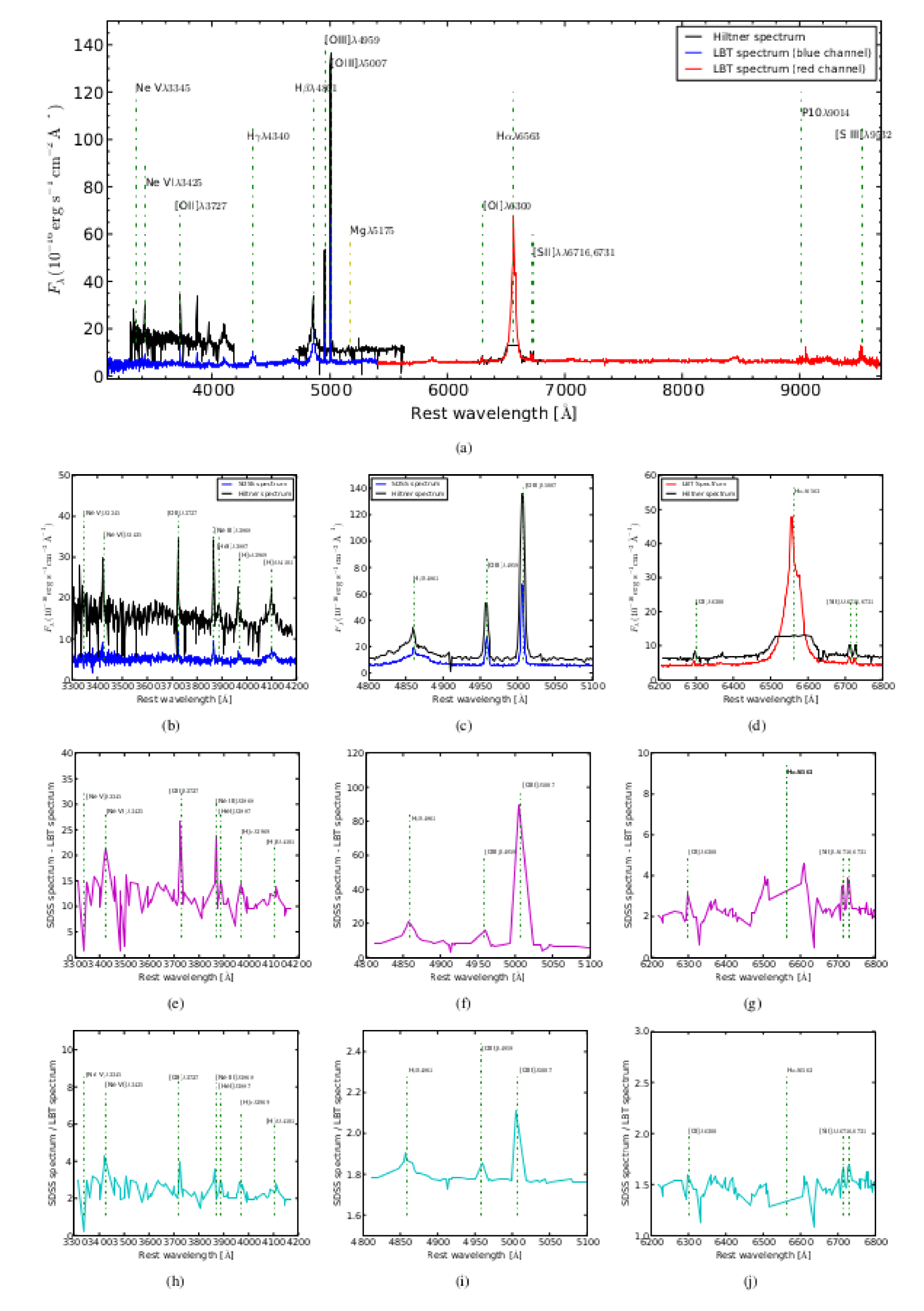15, where the continuum level of J0354 taken with the Hiltner telescope is higher than the LBT spectrum for the same source, and the emission lines of their observation are more intense than our observation. Additionally, Grupe, Pradhan & Frank (2005) report line fluxes of [[O iii] $\lambda 4959$ and $\lambda 5007$ as $(130\pm 6)$ and $(413\pm 15)\times 10^{-16}\mathrm{erg}\ \mathrm{s}^{-1}\ \mathrm{cm}^{-2}$ , respectively. From the LBT data we obtain fluxes of the same lines as $(90)\times 10^{-16}\mathrm{erg}\ \mathrm{s}^{-1}\ \mathrm{cm}^{-2}$ and $(505)\times 10^{-16}\mathrm{erg}\ \mathrm{s}^{-1}\ \mathrm{cm}^{-2}$ , respectively. The comparison shows that the [O iii] $\lambda 5007$ line varies by a factor of almost 50%.

5.7 GALEXASC J015328.23+260938.5

GALEXASC J015328.23+260938.5 (henceforward J0153) is the second source that is not covered by the SDSS survey. This source is present in the Infrared Astronomy Satellite (IRAS) Point Source Catalogue (Beichman et al., 1988, using the name IRAS 01506+2554) and in the 2nd XMM-Newton Serendipitous Source Catalog (Memola et al., 2007; Noguchi, Terashima & Awaki, 2009, using the name 2XMM J015328.4+26093). From the IRAS survey, we know the flux density at two wavelengths, 60 and 100 microns, to be 0.5777 & 1.144 Jy, respectively. In addition to our LBT observations (see Fig. 16) a spectrum of J0153 has been obtained by Zhou et al. (2002) in February 2002 with the Zeiss universal spectrograph located at the Beijing Observatory 2.16 m telescope, with a slit width of 2 $\aas@@fstack{\prime\prime}$ 5 and seeing disk of 2 $\aas@@fstack{\prime\prime}$ 5. Moreover, the spectral resolution determined on the night sky is $5.2\AA$ FWHM. They also found that J0153 is a radio-loud quasar with very strong Fe ii emission lines, for the far- and near-infrared luminosity, they found $\mathrm{{L}_{FIR}}\approx{10}^{12.7}\ \mathrm{L}_{\sun}$ and $\mathrm{{L}_{NIR}}\approx{10}^{12.5}\ \mathrm{L}_{\sun}$ .
J0153 is one of 30 galaxies that Combes et al. (2011) study to follow the galaxy evolution and especially the star formation efficiency (SFE) using CO lines. They find that the SFE of this source is $>$ 802 ( $\mathrm{{L}_{\sun}}/\mathrm{{M}_{\sun}}$ ) which is 4.7 times higher than the local ultra-luminous infrared galaxies (ULIRGs) (170 $\mathrm{{L}_{\sun}}/\mathrm{{M}_{\sun}}$ ), indicating highly efficient star formation activity.

5.8 SDSS J034740.18+010514.0

SDSS J034740.18+010514.0 (henceforth J0347) was mentioned first time in a study for high-luminosity sources (Low et al., 1988, using the name IRAS 03450+0055) and classified as quasar. In Hewitt & Burbidge (1991) J0347 was classified as S1 galaxy by Véron-Cetty & Véron (2006) as S1.5. With $\mathrm{{L}_{FIR}}\approx{10}^{10.2}$ Low et al. (1988) and Low et al. (1989) find J0347 to have the lowest luminosity among other quasars in their sample, additionally they find that this source has an extremely red optical continuum. 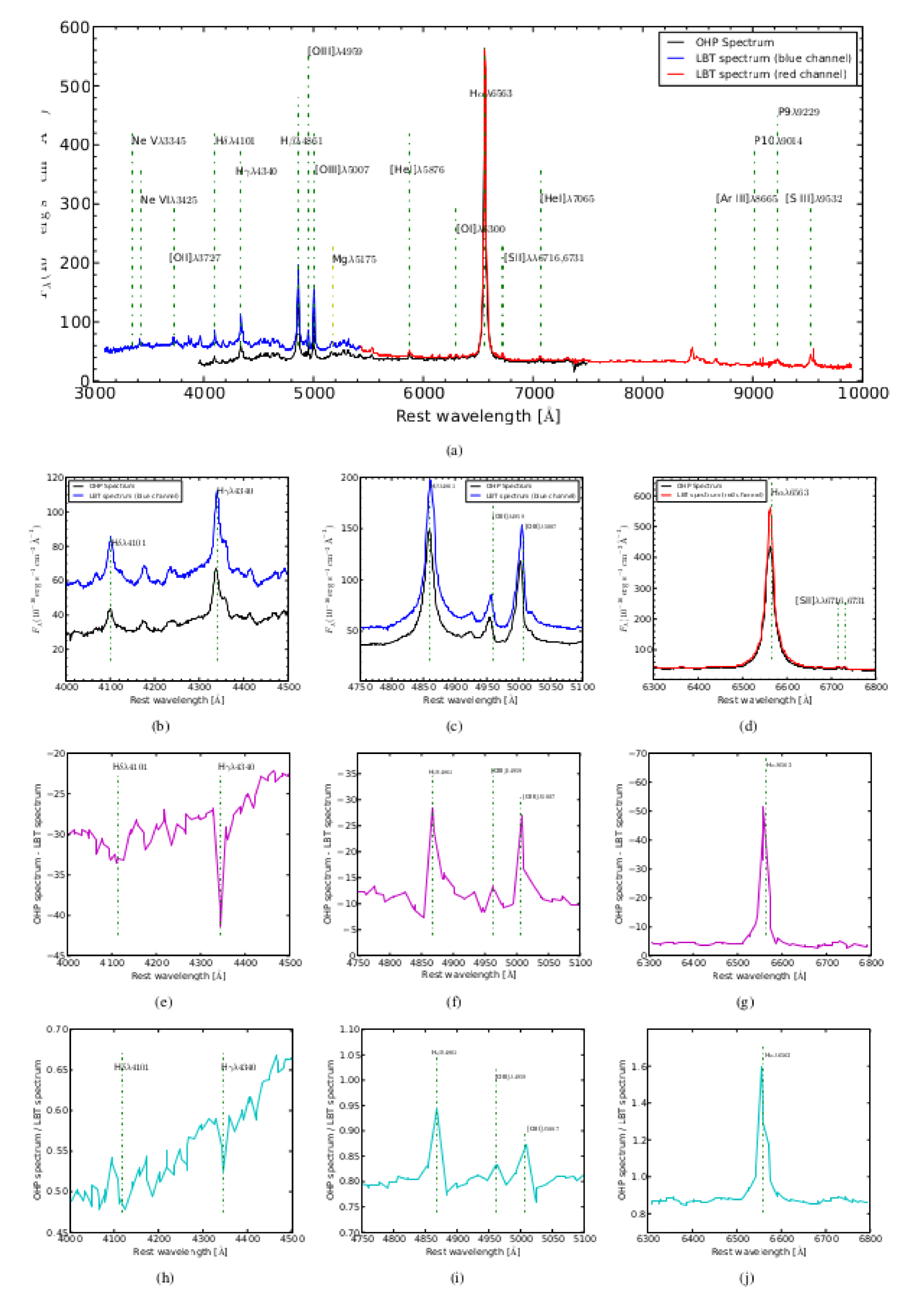Since no SDSS spectroscopic observations are available for this object, we used spectroscopic data taken on 21 September 2003 with the CARELEC spectrograph attached to the 1.93m telescope of the Observatoire de Haute-Provence (OHP) with a $2\arcsec$ slit under $2.5\arcsec$ seeing.
Giannuzzo & Stirpe (1996) search for variability in a sample of 12 narrow line Seyfert 1 galaxies, including J0347. They find 10 of these sources to be variable in the flux of the optical permitted lines over a period of one year and also found variation in the continuum level. The variability ratio they find in the permitted lines $\mathrm{H\beta}$ and $\mathrm{H\alpha}$ is 4.58 and 0.599 respectively.
We list measurements of the continuum flux from SDSS photometry as well as from OHP and LBT spectroscopy in Tab. LABEL:fig:variab. Line flux measurements are presented in Tab. 9 (see also plots in Fig. 17).

Table 6: Median and median deviations for the variability in the continuum & emission lines.

Type	Continuum		Narrow
			Emission lines
	$\mu$	$d\mu$	$\mu$	$d\mu$
BLS1& QSO	39.0	17.0	30.0	10.5
S2 & NLS1	27.0	9.0	15.0	6.0

Notes: $\mu$ are the median values, $d\mu$ the median deviations as defined in the text.

Table 7: The T-test statistic for the variability in the continuum & emission lines.

Type	Continuum					Emission lines
	n	$\overline{\chi}$	$\sigma$	df	T-value	n	$\overline{\chi}$	$\sigma$	df	T-value
BLS1& QSO	42	42.25	20.76	75	3.38	18	29.48	10.71	33	4.25
S2 & NLS1	35	29.51	11.72	75	3.38	17	15.51	8.67	33	4.25

Notes: Here $n$ denotes the number of sample elements, $\overline{\chi}$ are the sample mean values, $\sigma$ the sample standard deviations, $df$ the degrees of freedom followed by the corresponding T-values.

6 Discussion

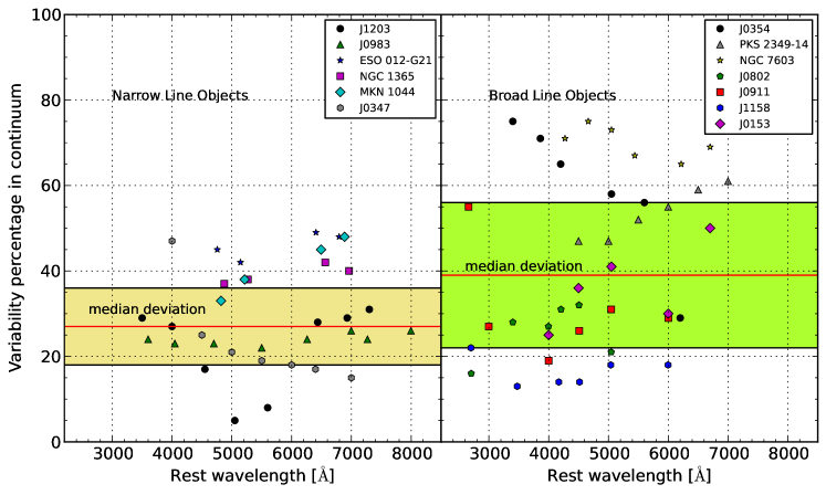
Our study allows us to compare the continuum and line variability of two different source samples with different spectroscopic identifications that by themselves imply a different degree of activity. We find that the Seyfert 2/NLS 1 sample shows in general a smaller degree of variability compared to the BLS1 and QSO sample. In the following we probe the significance of this difference and present a possible physical interpretation of the observed phenomenon. We extend the data on the continuum variability with multi epoch information on ESO 012-G21, NGC 1365, and MKN 1044 from Giannuzzo & Stirpe (1996), NGC 7603 from Kollatschny, Bischoff & Dietrich (2000) and PKS 2349-14 from Kollatschny, Zetzl & Dietrich (2006a). We extended the data on multi epoch line variability with ESO 012-G21, NGC 1365 and MKN 1044 from Giannuzzo & Stirpe (1996).

6.1 Probing the degree of variability

Based on our detailed study of 18 sources (see Tab. LABEL:all_sources1, Tab. 8 and captions in Figs. 6 and 7) we find that there are significant differences in variability between S2&NLS1 (8) sources and BLS1&QSO (10) sources. This applies both for the continuum and the emission lines. In the following we discuss the relative variability $\Delta_{max}$ as the maximum difference $\delta_{max}$ with respect to the maximum value $S_{max}$ , i.e. $\Delta_{max}=\delta_{max}/S_{max}$ in (i.e. dependent on the inter-calibration uncertainties which are the same for both source classes). Correction for relative measurement uncertainties $\sigma$ of the order of 10% results in

\Delta_{max,corr.}=\sqrt{\Delta_{max}^{2}-\sigma^{2}}

(2)

We find that the BLS1&QSO have stronger variablity than S2&NLS1. Ai et al. (2013a) came to the same conclusion: NLS1 have a systematically lower degree of variability if compared to BLS1 sources. This is in agreement with the existing anti-correlation between AGNs variability and Eddington ratio Meusinger, Hinze & de Hoon (2011); Zuo et al. (2012). Other authors (e.g., Webb & Malkan, 2000) concluded from variability studies that the blue part of AGN spectra is relatively stronger variable than the red part. For our study we show this result in Fig. 6. We notice that for J0354 and J0911 the variability in the blue part of the continuum is, larger than the variability in the red part.

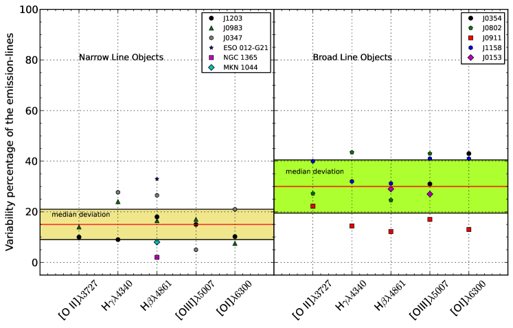
To judge on the difference between the two source samples in their continuum and line variability we calculated the median and median deviation as well as the mean and standard deviation. We also chose the median since we do not know ab-initio if we have normal distributions. Here, the median deviation is defined as the median of the absolute differences between the median and the sample values. The median deviation is usually smaller than the standard deviation as it is less sensitive with respect to outliers. From Tab. LABEL:t-test1 and Figs. 6 and 7 we find that the median degree of continuum variability is 27% $\pm$ 9% for the S2/NLS1 and 39% $\pm$ 17% for the BLS1/QSO sources. For the median line variability we find 15% $\pm$ 6% for the S2/NLS1 and 30% $\pm$ 11% for the BLS1/QSO sources. Furthermore, we find that the median values are separated by about one median deviation.

Table 8: The variability percentage in continuum at rest wavelength 5100Åand

\mathrm{H\beta}

, for AGNs taken from reverberation mapping (light curve).

Sources	Cont. 5100Å	$\mathrm{H\beta}$	Type	References
	%	%
Mrk 335	34	24	NLS1	1,2
Mrk 6	36	25	NLS1	1
3C 120	57	40	BLS1	1
Ark 120	48	47	BLS1	1
Mrk 590	43	50	BLS1	1

References. (1) Peterson et al. (1998), (2) Grier et al. (2012).

6.1.1 Robustness of the separation

Results for narrow and broad line components: In Fig. 7 we show the results for the combined narrow and broad line recombination line fluxes in order to compare the data with literature values. However, the difference in the variability behavior between the narrow line and the broad line sources (with 15% $\pm$ 6% and 30% $\pm$ 11%, respectively) also holds if we investigate the narrow line and broad line components we obtained from fitting the hydrogen recombination lines (see Tab. LABEL:narr_bro). Here the median value for the variability of the narrow line objects J0347, J1203 and J0938 of 20 $\pm$ 4 lies well below the median result for the broad line objects of 41 $\pm$ 8 derived from the 4 objects J1158, J0911, J0002 and J0153. Although the separation into the two different source classes has been done using an overall line width criterion, we find that the difference is also present if we look at the NLR and BLR line components separately (see discussion in section 6.3).

Statistical considerations: For the BLS1/QSO sample we see the tendency in some sources for the variability to be up to 20% stronger in the blue (3000Å) compared to the red (close to 6000Å). However, this tendency is not equally well fullfiled for all sources and rather weak with respect to the overall variability range from about 20% to 70%. However, here we are more interested in the overall continuum and line variability. Both are estimated for different sources and in different lines or spectral regions of the continuum, which are all subject to different wavelength and line strength dependant calibration uncertainties. Hence, we assume that for the two source samples the variability estimates are sufficiently independent, and can be represented by a mean distribution. In this case we can apply a T-test (Senn & Richardson, 1994) to determine the probability that the data sets from both the continuum and line variation originate from different distributions. The relevant test quantities are given in Tab. LABEL:t-test2.
We applied a T-test for two sample experimental statistics for independent groups. The T-value was calculated via

T=\frac{\overline{\chi_{1}}-\overline{\chi_{2}}}{\sigma_{diff}}~{}~{}.

(3)

The standard error of the difference we calculated via

\sigma_{diff}=\sqrt{\sigma^{2}_{\overline{\chi_{1}}}+\sigma^{2}_{\overline{\chi_{2}}}}~{}~{}.

(4)

Since we do not know the population standard deviation we use the sample standard deviation to estimate the standard error:

\sigma_{\overline{\chi}}=\frac{\sigma}{\sqrt{n}}~{}~{},

(5)

$n$ being the number of sample elements. The number of degrees of freedom $df$ as used for two independent groups we obtained as

df=(n_{1}-1)+(n_{2}-1)~{}~{}~{}.

(6)

The probabilities that describe the matching of the two samples are tabulated (Senn & Richardson, 1994) as a function of the T-values and the degrees of freedom $df$ . We find that the continuum and line variability of the BLS1 and QSO sample originated with a better than 99.9% probability from a different distribution compared to the Seyfert 2 and NLS1 sample.

Comparison to other samples: The separation between the narrow line and the broad line sources is best fulfilled for the line variation. As shown in Tab. 8 our results are very much consistent with those for a set of NLS1 and BLS1 sources obtained from reverberation measurements carried out by Peterson et al. (1998) and Grier et al. (2012).
The findings for our small sample are also in full agreement with the results of a comparative study of the optical/ultraviolet variability of NLS1 and BLS1-type sources by Ai et al. (2013b) (based on 55 NLS1- and 108 BLS1-type nuclei). This underlines the representative character of our sample. The authors show that the majority of NLS1-type objects exhibit significant variability on timescales from about 10 days up to a few years, but on average their variability amplitudes are much smaller compared to BLS1-type sources (see also, Yip et al., 2009; Barth et al., 2014). Hence, in summary, we assume that the difference in continuum and line variability between the two samples is sufficiently significant to search for a physical explanation for the phenomenon.

6.2 Accretion dominated variability

Here we investigate how the difference in narrow line variability between the objects with spectra dominated by narrow lines and broad lines is linked to the continuum variations of the active nuclei in the different samples.

In the following we denote with $\Delta$ differentiation with respect to the different samples, i.e. $\Delta=\frac{d}{d~{}~{}sample}$ . If the variability is due to mass accretion $\frac{d}{dt}M$ onto a super-massive black hole with mass $M$ we can write the continuum luminosity $L_{cont.}$ as

L_{cont.}\propto M\times\frac{d}{dt}M~{}~{}.

(7)

The expected difference in continuum variability between the samples can then be expressed as

\Delta L_{cont.}\propto\Delta M\times\frac{d}{dt}M+M\times\Delta\frac{d}{dt}M~{}~{}~{}.

(8)

For recombination lines the variation of the nuclear continuum results in a variation of the number of atomic species that reach the next higher state of ionization out of which they can recombine. For collisionally excited states this next higher state of ionization is the state in which they can be observed at low densities emitting forbidden narrow line radiation. In the following we use the case of the recombination lines to discuss the effect of the reverberation. Since we are mainly interested in the variation of the narrow line luminosity $L_{line}$ as a reverberation response to the variations in continuum luminosity we can write:

L_{line}\propto\frac{h\nu_{line}}{\langle hv\rangle}\frac{\alpha_{eff}}{\alpha_{B}}\frac{d}{dt}M=\xi\frac{d}{dt}M;

(9)

Here $\nu_{line}$ is the line frequency, $\alpha_{eff}$ and $\alpha_{B}$ are the effective and Menzel’s case $B$ specific recombination coefficients and $\langle hv\rangle$ denotes the mean energy per photon. Through the latter the combined coefficient $\xi$ depends on the ration between the total illuminated cross-section $A_{C}$ and ionized volume $V_{C}$ of the reverberating clouds in a single galactic nucleus. This ratio results in a size $l$ of the reverberating volume which has a square root dependency on the continuum luminosity:

\xi\propto\frac{V_{C}}{A_{C}}\propto l\propto\sqrt{L_{cont.}}~{}~{}~{}.

(10)

Therefore, combining the above equations for the line luminosity we can write:

L_{line}\propto\sqrt{M}(\frac{d}{dt}M)^{\frac{3}{2}}~{}~{}~{}.

(11)

The expected difference in line variability between the samples can then be expressed as

\Delta L_{line}\propto\frac{1}{2}M^{-\frac{1}{2}}\Delta M(\frac{d}{dt}M)^{\frac{3}{2}}+M^{\frac{1}{2}}\frac{3}{2}(\frac{d}{dt}M)^{\frac{1}{2}}(\Delta\frac{d}{dt}M)~{}~{}~{}.

(12)

We now assume that - as a second order derivative - the variation $\Delta\frac{d}{dt}M$ of the accretion stream onto the super-massive black holes from sample to sample is small and a finite difference $\Delta M$ in total mean black hole mass per sample needs to be considered. In such a scenario, the strength of the accretion stream as such is the dominant quantity for the variations in continuum and line luminosity between between different sample members and the two sources sample in general. We can then neglect the second terms in equations and and write for the difference in continuum and line luminosity:

\Delta L_{cont.}\propto\Delta M\times\frac{d}{dt}M\propto\frac{d}{dt}M

(13)

\Delta L_{line}\propto\Delta M(\frac{d}{dt}M)^{\frac{3}{2}}\propto(\frac{d}{dt}M)^{\frac{3}{2}}~{}~{}~{}.

(14)

Hence the increase in activity in continuum and line emission is due to the difference in $\Delta M$ between the samples, however, there is an additional modulation for the variability of the line emission that is a function of $\frac{d}{dt}M$ . Combining these results we find:

\Delta L_{line}\propto(\Delta L_{cont.})^{\frac{3}{2}}~{}~{}~{}.

(15)

This simple relation was obtained by assuming that the difference in accretion streams between the two samples is - to first order - negligible. The accretion stream onto the super-massive black hole is probably closely tied to the properties of the interstellar matter in its immediate vicinity. Hence, it may be different from source to source and may not strongly depend on the mass of the central super-massive black hole. However, if $\Delta\frac{d}{dt}M$ needs to be considered it will have an influence on the general trend of the derived relation (i.e the overall slope and curvature of the trend). In fact, it may be responsible for part of the scatter of data points about this relation. However, we assume the second order derivative to be of lesser importance than the first order derivatives. This is supported by the fact that the general trend of the distribution of data points in Fig. 8 is well described.

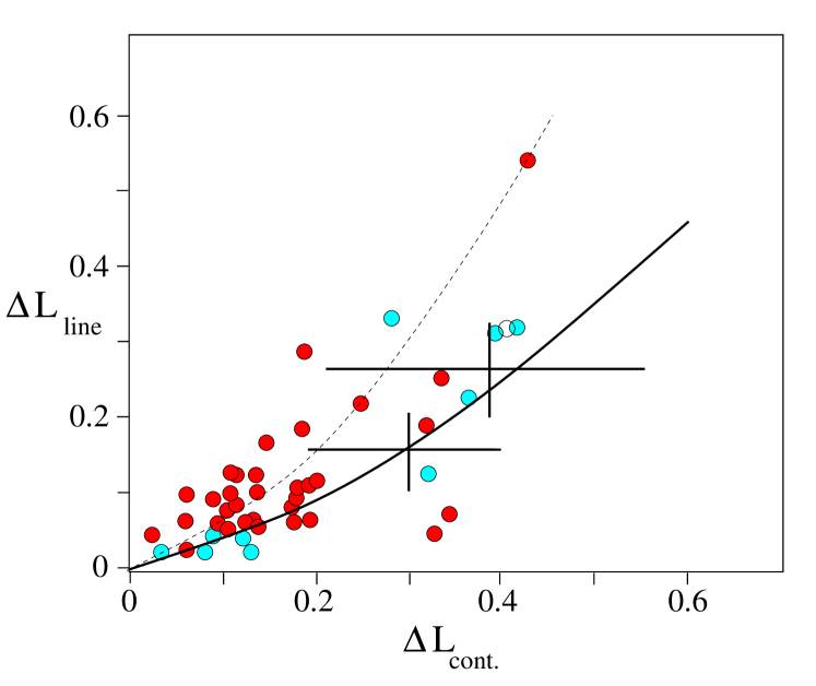
Looking at the median and mean values for the different samples in Tabs. LABEL:t-test1 and LABEL:t-test2 we find that this condition described by equation 15 is to first order fullfiled to within about 15% : For the means of the continuum variability we find $(39/30)^{\frac{3}{2}}=1.5$ whereas the measured ratio of the means of the line variability is $27/15=1.8$ . For the median values of the continuum variability we find $(42/35)^{\frac{3}{2}}=1.3$ whereas the measured ratio of the median values of the line variability is $29/16=1.8$ . This proportionality relation between the continuum and narrow line variability is demonstrated in Fig. 8 and discussed in the following section.

6.3 NLR response to the nuclear continuum variability

In Fig. 8 the black crosses represent the median values and their uncertainties as shown in Figs. 6 & 7. In this plot the curved lines represent the relation $\Delta L_{line}=\epsilon(\Delta L_{cont.})^{\frac{3}{2}}$ , with $\epsilon$ =1.0 for the thick straight line which follows our data surprisingly well. There are two main contributers $\eta_{star}$ and $\eta_{fill}$ to that value such that $\epsilon=\frac{\eta_{star}}{\eta_{fill}}$ . For our sample, of the order of 50% of the continuum flux density is likely to be due to the stellar continuum, which is not variable on the time scales discussed here. For more luminous objects this may be of the order of 20% (Kollatschny, Zetzl & Dietrich, 2006b). This indicates that the pure nuclear continuum variability which is not contaminated by stellar flux may in general be larger by up to 50%. This results in a value of $\eta_{star}\sim$ 1.9 (dashed line in Fig. 8). However, the covering factor $\eta_{fill}$ of the clouds that are illuminated by the nucleus can be of the same order of magnitude. Hence, with a considerable scatter, $\epsilon$ may in fact be close to unity, such that the bold black line in Fig. 8 that matches the observed data is an acceptable representation of the relation between the continuum and narrow line variability.

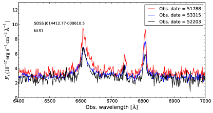
We have carried out the interpretation of the line response using the reverberation formalism. This is usually applied to broad lines only and used to derive the size of the BLR, making use of well sampled continuous light curves of the continuum and broad line emission, which are then cross-correlated. In Fig. 8 we compare our finding with variability data from different broad line QSO samples. The blue filled dots are QSO variability data from the sample listed in Tab.6 by Kollatschny, Zetzl & Dietrich (2006b) the red filled dots are data from Peterson et al. (2004) and Kaspi et al. (2000) as listed in Tab.8 by Kollatschny, Zetzl & Dietrich (2006b). The comparison shows that the relation also holds for reverberation response of the broad line QSOs. With the additional literature data Fig. 8 now comprises a total of 61 sources. In the work we present here, however, the line response that we monitored in our small sample is dominated by forbidden narrow line emission. Only the H $\beta$ line allows a separation between the broad and narrow line contribution. However, the median and mean derived from the BLR component only is in good agreement with the overall result. We base our investigation on typically 2 measurements over a baseline in time of the order of 10 years (see Tab. LABEL:narr_bro). Reverberation response of the NLR based on measurements over 5-8 years has also been reported for the radio galaxy 3C390.3 (Clavel & Wamsteker, 1987) and for the S1 galaxy NGC 5548 (Peterson et al., 2013). Within the SDSS survey one can also find example of multi-epoch observations that are consistent with this picture. In Fig. 18 we show three epoch SDSS spectra for the NLS1 sources J014412 and J022205. The variability estimates places them well into Fig. 8.

Variability on time scale of years already sets an upper limit to the size of the corresponding region. Since the variability is rather significant, the line flux contribution of that region is also high. While there is a density and temperature gradient towards the nuclear position (Ogle et al., 2000; Penston et al., 1990; Morse et al., 1995) one also finds that the surface brightness distribution of the NLR flux is very much centrally peaked. The size of the NRL is luminosity dependant(Schmitt et al., 2003), however, the inspection of high angular resolution HST scans across S1 and S2 nuclei shows that the unresolved central peak may contain 50% or more of the more extended nuclear forbidden line flux (Bennert et al., 2006a, b). Peterson et al. (2013) find for NGC 5548 that 94% of the NLR emission arises from within 18pc (54 ly). Ogle et al. (2000) derive a density profile of r^-2 and Walsh et al. (2008) find that the [S II] line ratio indicates a radial stratification in gas density, with a sharp increase within the inner 10-20 pc, in the majority of the Type 1 (broad-lined) objects.

Hence, the main response to the continuum variation must therefore originate in a rather compact region with a diameter of the order of 10 light years. This is in good agreement with the finding for 3C390.3 (Clavel & Wamsteker, 1987) and NGC 5548 (Peterson et al., 2013). Since this formalism fully explains the reverberation of the line emission with respect to the continuum variation (with a surprisingly close proportionality; see Fig. 8), this suggests that the region illuminated by the nucleus is almost fully spatially overlapping with the responding line emitting region. Hence, at larger distance the NLRs then show a much weaker response to the continuum variability most likely due to a combination of a lower overall luminosity and a lower volume filling factor. The close correlation to the non-stellar nuclear continuum variability also implies that for the sources we investigated there are no other significant sources (i.e. star formation, extra nuclear shocks) but the nuclear radiation field that contributes substantially to the line emission of the reverberating region.

7 Conclusions

We investigated a sample of 18 sources. For 8 objects in Tab. LABEL:all_sources1 we performed a detailed analysis spectroscopy over the available optical wavelength range. For 10 sources we obtained suitable multi epoch line and continuum data from the literature (see Tab. 8 and Figs. 6 and 7) covering time scales from 5 to 10 years. Fig. 8 demonstrates that our findings describe the variability characteristics of a total of 61 sources. From the line and continuum variability of these active galactic nuclei we find the following consistent picture that explains the differences between the Seyfert 2/NLS 1 and the BLS1 and QSO sample: The line luminosity $L_{line}$ can be described as a reverberation response to the continuum luminosity $L_{cont}$ . In good agreement results of previous studies (references in section 6.3) we find that the bulk of the NLR emission arises from within 10-20 light years and shows a reverberation response to variability of the nucleus. The differences in variability do not require a variation of the accretion rate $\Delta\frac{d}{dt}M$ between the two samples. It is mainly the difference in black hole mass $\Delta M$ that is responsible for the difference between the samples. The increased variability of the line emission can fully be explained by the dependency on the accretion rate $\frac{d}{dt}M$ .

Acknowledgments

Y.E. Rashed is supported by the German Academic Exchange Service (DAAD) and by the Iraqi ministry of higher education and scientific research. Y.E.R. wants to thank Dr. M.-P. Véron-Cetty for providing us with an optical spectra for one of the source. Macarena García-Marín is supported by the German federal department for education and research (BMBF) under the project number 50OS1101. Gerold Busch is member of the Bonn-Cologne Graduate School of Physics and Astronomy.

The spectroscopic observations reported here were obtained at the LBT Observatory, a joint facility of the Smithsonian Institution and the University of Arizona. LBT observations were obtained as part of the Rat Deutscher Sternwarten guaranteed time on Steward Observatory facilities through the LBTB cooperation. This paper uses data taken with the MODS spectrographs built with funding from NSF grant AST-9987045 and the NSF Telescope System Instrumentation Program (TSIP), with additional funds from the Ohio Board of Regents and the Ohio State University Office of Research. The Sloan Digital Sky Survey is a joint project of the University of Chicago, Fermilab, the Institute for Advanced Study, the Japan Participation Group, Johns Hopkins University, the Max-Planck-Institute for Astronomy, the Max-Planck-Institute for Astrophysics, New Mexico State University, Princeton University, the United States Naval Observatory, and the University of Washington. Apache Point Observatory, site of the SDSS, is operated by the Astrophysical Research C consortium. Funding for the project has been provided by the Alfred P. Sloan Foundation, the SDSS member institutions, NASA, the NSF, the Department of Energy, the Japanese Monbukagakusho, and the Max-Planck Society. The SDSS Web site is http://www.sdss.org.

References

Abazajian et al. (2009) Abazajian K. N. et al., 2009, ApJS, 182, 543
Adelman-McCarthy et al. (2008) Adelman-McCarthy J. K. et al., 2008, ApJS, 175, 297
Adelman-McCarthy & et al. (2009) Adelman-McCarthy J. K., et al., 2009, VizieR Online Data Catalog, 2294, 0
Adelman-McCarthy & et al. (2011) Adelman-McCarthy J. K., et al., 2011, VizieR Online Data Catalog, 2306, 0
Ai et al. (2013a) Ai Y. L., Yuan W., Zhou H., Wang T. G., Dong X.-B., Wang J. G., Lu H. L., 2013a, AJ, 145, 90
Ai et al. (2013b) Ai Y. L., Yuan W., Zhou H., Wang T. G., Dong X.-B., Wang J. G., Lu H. L., 2013b, AJ, 145, 90
Allen et al. (2011) Allen J. T., Hewett P. C., Maddox N., Richards G. T., Belokurov V., 2011, MNRAS, 410, 860
Angione & Smith (1972) Angione R. J., Smith H. J., 1972, in IAU Symposium, Vol. 44, External Galaxies and Quasi-Stellar Objects, Evans D. S., Wills D., Wills B. J., eds., p. 171
Antonucci (1993) Antonucci R., 1993, ARAA, 31, 473
Barth et al. (2014) Barth A. J., Voevodkin A., Carson D. J., Woźniak P., 2014, AJ, 147, 12
Beichman et al. (1988) Beichman C. A., Neugebauer G., Habing H. J., Clegg P. E., Chester T. J., 1988, in Infrared astronomical satellite (IRAS) catalogs and atlases. Volume 1: Explanatory supplement
Bennert et al. (2006a) Bennert N., Jungwiert B., Komossa S., Haas M., Chini R., 2006a, A&A, 459, 55
Bennert et al. (2006b) Bennert N., Jungwiert B., Komossa S., Haas M., Chini R., 2006b, A&A, 456, 953
Boroson & Green (1992) Boroson T. A., Green R. F., 1992, ApJS, 80, 109
Bothun et al. (1982) Bothun G. D., Chanan G. A., Romanishin W., Margon B., Schommer R. A., 1982, ApJ, 257, 40
Brotherton et al. (1994) Brotherton M. S., Wills B. J., Steidel C. C., Sargent W. L. W., 1994, ApJ, 423, 131
Bruzual & Charlot (2003) Bruzual G., Charlot S., 2003, MNRAS, 344, 1000
Chanan, Downes & Margon (1981) Chanan G. A., Downes R. A., Margon B., 1981, ApJL, 243, L5
Cid Fernandes & Sodre (2000) Cid Fernandes R., Sodre L., 2000, in Bulletin of the American Astronomical Society, Vol. 32, American Astronomical Society Meeting Abstracts #196, p. 751
Clavel & Wamsteker (1987) Clavel J., Wamsteker W., 1987, ApJL, 320, L9
Combes et al. (2011) Combes F., García-Burillo S., Braine J., Schinnerer E., Walter F., Colina L., 2011, A&A, 528, A124
Corbin (1997) Corbin M. R., 1997, ApJS, 113, 245
Darling & Giovanelli (2002) Darling J., Giovanelli R., 2002, AJ, 124, 100
Dong et al. (2011) Dong X.-B., Wang J.-G., Ho L. C., Wang T.-G., Fan X., Wang H., Zhou H., Yuan W., 2011, ApJ, 736, 86
Gaskell (2008) Gaskell C. M., 2008, in Revista Mexicana de Astronomia y Astrofisica Conference Series, Vol. 32, Revista Mexicana de Astronomia y Astrofisica Conference Series, pp. 1–11
Giannuzzo & Stirpe (1996) Giannuzzo E. M., Stirpe G. M., 1996, A&A, 314, 419
Gibson et al. (2009) Gibson R. R. et al., 2009, ApJ, 692, 758
Grier et al. (2012) Grier C. J. et al., 2012, ApJ, 755, 60
Grupe, Pradhan & Frank (2005) Grupe D., Pradhan A. K., Frank S., 2005, AJ, 130, 355
Guo & Gu (2014) Guo H., Gu M., 2014, ApJ, 792, 33
Haas et al. (2007) Haas M., Siebenmorgen R., Pantin E., Horst H., Smette A., Käufl H.-U., Lagage P.-O., Chini R., 2007, A&A, 473, 369
Haddad & Vanderriest (1991) Haddad B., Vanderriest C., 1991, A&A, 245, 423
Hewett & Wild (2010) Hewett P. C., Wild V., 2010, MNRAS, 405, 2302
Hewitt & Burbidge (1991) Hewitt A., Burbidge G., 1991, ApJS, 75, 297
Hogg (1999) Hogg D. W., 1999, ArXiv Astrophysics e-prints
Hook et al. (1994) Hook I. M., McMahon R. G., Boyle B. J., Irwin M. J., 1994, MNRAS, 268, 305
Hutchings, Campbell & Crampton (1982) Hutchings J. B., Campbell B., Crampton D., 1982, ApJL, 261, L23
Inada et al. (2012) Inada N. et al., 2012, AJ, 143, 119
Kaspi et al. (2007) Kaspi S., Brandt W. N., Maoz D., Netzer H., Schneider D. P., Shemmer O., 2007, ApJ, 659, 997
Kaspi et al. (2000) Kaspi S., Smith P. S., Netzer H., Maoz D., Jannuzi B. T., Giveon U., 2000, ApJ, 533, 631
Kollatschny, Bischoff & Dietrich (2000) Kollatschny W., Bischoff K., Dietrich M., 2000, A&A, 361, 901
Kollatschny, Zetzl & Dietrich (2006a) Kollatschny W., Zetzl M., Dietrich M., 2006a, A&A, 454, 459
Kollatschny, Zetzl & Dietrich (2006b) Kollatschny W., Zetzl M., Dietrich M., 2006b, A&A, 454, 459
Komossa (2008) Komossa S., 2008, in Revista Mexicana de Astronomia y Astrofisica Conference Series, Vol. 32, Revista Mexicana de Astronomia y Astrofisica Conference Series, pp. 86–92
Kovačević, Popović & Dimitrijević (2010) Kovačević J., Popović L. Č., Dimitrijević M. S., 2010, ApJS, 189, 15
Low et al. (1988) Low F. J., Cutri R. M., Huchra J. P., Kleinmann S. G., 1988, ApJL, 327, L41
Low et al. (1989) Low F. J., Cutri R. M., Kleinmann S. G., Huchra J. P., 1989, ApJL, 340, L1
Lundgren et al. (2009) Lundgren B. F. et al., 2009, ApJ, 698, 819
Margon, Chanan & Downes (1982) Margon B., Chanan G. A., Downes R. A., 1982, ApJL, 253, L7
Markwardt (2009) Markwardt C. B., 2009, in Astronomical Society of the Pacific Conference Series, Vol. 411, Astronomical Data Analysis Software and Systems XVIII, Bohlender D. A., Durand D., Dowler P., eds., p. 251
McMahon et al. (2002) McMahon R. G., White R. L., Helfand D. J., Becker R. H., 2002, ApJS, 143, 1
Memola et al. (2007) Memola E. et al., 2007, A&A, 465, 759
Meusinger, Hinze & de Hoon (2011) Meusinger H., Hinze A., de Hoon A., 2011, A&A, 525, A37
Meusinger & Weiss (2013) Meusinger H., Weiss V., 2013, A&A, 560, A104
Morse et al. (1995) Morse J. A., Wilson A. S., Elvis M., Weaver K. A., 1995, ApJ, 439, 121
Noguchi, Terashima & Awaki (2009) Noguchi K., Terashima Y., Awaki H., 2009, ApJ, 705, 454
Ogle et al. (2000) Ogle P. M., Marshall H. L., Lee J. C., Canizares C. R., 2000, ApJL, 545, L81
Osterbrock (1985) Osterbrock D. E., 1985, PASP, 97, 906
Osterbrock, Fulbright & Bida (1997) Osterbrock D. E., Fulbright J. P., Bida T. A., 1997, PASP, 109, 614
Osterbrock et al. (1996) Osterbrock D. E., Fulbright J. P., Martel A. R., Keane M. J., Trager S. C., Basri G., 1996, PASP, 108, 277
Osterbrock & Pogge (1985) Osterbrock D. E., Pogge R. W., 1985, ApJ, 297, 166
Penston et al. (1990) Penston M. V. et al., 1990, A&A, 236, 53
Peterson (2001) Peterson B. M., 2001, in Advanced Lectures on the Starburst-AGN, Aretxaga I., Kunth D., Mújica R., eds., p. 3
Peterson et al. (2002) Peterson B. M. et al., 2002, ApJ, 581, 197
Peterson et al. (1984) Peterson B. M., Crenshaw D. M., Meyers K. A., Byard P. L., Foltz C. B., 1984, ApJ, 279, 529
Peterson et al. (2013) Peterson B. M. et al., 2013, ApJ, 779, 109
Peterson et al. (2004) Peterson B. M. et al., 2004, ApJ, 613, 682
Peterson & Gaskell (1986) Peterson B. M., Gaskell C. M., 1986, AJ, 92, 552
Peterson et al. (1998) Peterson B. M., Wanders I., Bertram R., Hunley J. F., Pogge R. W., Wagner R. M., 1998, ApJ, 501, 82
Pogge et al. (2010) Pogge R. W. et al., 2010, in Society of Photo-Optical Instrumentation Engineers (SPIE) Conference Series, Vol. 7735, Society of Photo-Optical Instrumentation Engineers (SPIE) Conference Series
Pogge et al. (2012) Pogge R. W. et al., 2012, in Society of Photo-Optical Instrumentation Engineers (SPIE) Conference Series, Vol. 8446, Society of Photo-Optical Instrumentation Engineers (SPIE) Conference Series
Ruan et al. (2014) Ruan J. J., Anderson S. F., Dexter J., Agol E., 2014, ApJ, 783, 105
Sánchez Almeida et al. (2011) Sánchez Almeida J., Aguerri J. A. L., Muñoz-Tuñón C., Huertas-Company M., 2011, ApJ, 735, 125
Schmitt et al. (2003) Schmitt H. R., Donley J. L., Antonucci R. R. J., Hutchings J. B., Kinney A. L., Pringle J. E., 2003, ApJ, 597, 768
Schneider et al. (2007) Schneider D. P. et al., 2007, AJ, 134, 102
Schneider et al. (2005) Schneider D. P. et al., 2005, AJ, 130, 367
Schneider et al. (2010) Schneider D. P. et al., 2010, AJ, 139, 2360
Senn & Richardson (1994) Senn S., Richardson W., 1994, Statistics in Medicine 13 (8), 785, 803
Shapovalova et al. (2010) Shapovalova A. I., Popović L. Č., Burenkov A. N., Chavushyan V. H., Ilić D., Kovačević A., Bochkarev N. G., León-Tavares J., 2010, A&A, 509, A106
Shirazi & Brinchmann (2012) Shirazi M., Brinchmann J., 2012, MNRAS, 421, 1043
Skrutskie et al. (2006) Skrutskie M. F. et al., 2006, AJ, 131, 1163
Spergel et al. (2003) Spergel D. N. et al., 2003, ApJS, 148, 175
Starling & Puchnarewicz (2001) Starling R. L. C., Puchnarewicz E. M., 2001, in Two Years of Science with Chandra
Stepanian & Afanas’ev (2011) Stepanian J. A., Afanas’ev V. L., 2011, Astrophysics, 54, 340
Stoughton et al. (2002) Stoughton C. et al., 2002, AJ, 123, 485
Urry & Padovani (1995) Urry C. M., Padovani P., 1995, PASP, 107, 803
Vanden Berk et al. (2004) Vanden Berk D. E. et al., 2004, ApJ, 601, 692
Véron-Cetty & Véron (2006) Véron-Cetty M.-P., Véron P., 2006, A&A, 455, 773
Walsh et al. (2008) Walsh J. L., Barth A. J., Ho L. C., Filippenko A. V., Rix H.-W., Shields J. C., Sarzi M., Sargent W. L. W., 2008, AJ, 136, 1677
Wang & Rowan-Robinson (2009) Wang L., Rowan-Robinson M., 2009, MNRAS, 398, 109
Wang et al. (2012) Wang T.-G., Zhou H.-Y., Komossa S., Wang H.-Y., Yuan W., Yang C., 2012, ApJ, 749, 115
Webb & Malkan (2000) Webb W., Malkan M., 2000, ApJ, 540, 652
Wilhite et al. (2005) Wilhite B. C., Vanden Berk D. E., Kron R. G., Schneider D. P., Pereyra N., Brunner R. J., Richards G. T., Brinkmann J. V., 2005, ApJ, 633, 638
Yang et al. (2013) Yang C.-W., Wang T.-G., Ferland G., Yuan W., Zhou H.-Y., Jiang P., 2013, ApJ, 774, 46
Yip et al. (2009) Yip C. W. et al., 2009, AJ, 137, 5120
York et al. (2000) York D. G. et al., 2000, AJ, 120, 1579
Zhang & Wang (2006) Zhang E.-P., Wang J.-M., 2006, ApJ, 653, 137
Zhang et al. (2010) Zhang S., Wang T.-G., Wang H., Zhou H., Dong X.-B., Wang J.-G., 2010, ApJ, 714, 367
Zhou et al. (2006) Zhou H., Wang T., Yuan W., Lu H., Dong X., Wang J., Lu Y., 2006, ApJS, 166, 128
Zhou et al. (2002) Zhou H.-Y., Wang T.-G., Zhou Y.-Y., Cheng-Li, Dong X.-B., 2002, ApJ, 581, 96
Zuo et al. (2012) Zuo W., Wu X.-B., Liu Y.-Q., Jiao C.-L., 2012, ApJ, 758, 104
Zuo et al. (2013) Zuo W., Wu X.-B., Liu Y.-Q., Jiao C.-L., 2013, in IAU Symposium, Vol. 290, IAU Symposium, Zhang C. M., Belloni T., Méndez M., Zhang S. N., eds., pp. 373–374

Table 9: The line fitting results for J0938, J1203, 1158, J0911, J0802, J0354, J0153, and J0347.

Sources	Em. lines	Ob. Wa.	Inst.1		Inst.2
			Flux	FWHM	Flux	FWHM
		Å	[ $10^{-16}\ \mathrm{erg}$	Å	[ $10^{-16}\ \mathrm{erg}$	Å
			$\mathrm{s}^{-1}\ \mathrm{cm}^{-2}$ ]		$\mathrm{s}^{-1}\ \mathrm{cm}^{-2}$ ]
			SDSS^a		LBT
J0938	[O ii] $\lambda$ 3727	$4102\pm 1$	$50.12\pm 2.39$	$5.66\pm 0.49$	$43.08\pm 2.38$	$6.05\pm 0.47$
	[Ne iii] $\lambda$ 3868	$4258\pm 1$	$11.28\pm 0.91$	$10.67\pm 0.93$	$7.97\pm 1.14$	$8.38\pm 0.79$
	H $\gamma$ $\lambda$ 4340	$4777\pm 1$	$25.18\pm 1.58$	$6.31\pm 0.88$	$18.95\pm 1.10$	$6.91\pm 0.71$
	He II $\lambda$ 4686	$5157\pm 2$	$8.50\pm 0.73$	$16.81\pm 1.12$	$4.04\pm 0.36$	$10.66\pm 0.87$
	H $\beta^{*}$ $\lambda$ 4861	$5350\pm 1$	$50.28\pm 2.54$	$5.61\pm 0.49$	$41.95\pm 2.83$	$5.91\pm 0.73$
	[O iii] $\lambda$ 5007	$5510\pm 1$	$45.06\pm 1.57$	$7.34\pm 0.57$	$37.43\pm 2.01$	$7.27\pm 0.66$
	[Fe vii] $\lambda$ 5721	$6298\pm 1$	$4.60\pm 0.39$	$10.56\pm 0.35$	$6.55\pm 1.11$	$11.74\pm 0.64$
	[Fe vii] $\lambda$ 6087	$6699\pm 1$	$11.55\pm 0.75$	$18.63\pm 0.51$	$11.19\pm 1.48$	$19.65\pm 0.72$
	[O i] $\lambda$ 6300	$6935\pm 1$	$4.94\pm 0.40$	$6.75\pm 0.41$	$5.30\pm 1.14$	$9.14\pm 0.83$
	H $\alpha$ $\lambda$ 6563	$7224\pm 1$	$208.83\pm 5.89$	$7.75\pm 0.57$	$164.56\pm 5.03$	$6.43\pm 0.61$
	[N ii] $\lambda$ 6583	$7246\pm 1$	$80.04\pm 2.57$	$7.77\pm 0.52$	$57.33\pm 2.70$	$6.17\pm 0.65$
	[S ii] $\lambda$ 6716	$7393\pm 1$	$28.90\pm 1.25$	$7.46\pm 0.54$	$23.08\pm 1.45$	$5.92\pm 0.52$
	[S ii] $\lambda$ 6731	$7409\pm 1$	$19.28\pm 0.96$	$7.15\pm 0.56$	$16.48\pm 1.32$	$6.02\pm 0.51$
			SDSS		LBT
J1203	[Ne v] $\lambda$ 3345	$3898\pm 1$	$20.42\pm 1.41$	$5.75\pm 0.22$	$27.82\pm 1.02$	$5.18\pm 0.31$
	[Ne vi] $\lambda$ 3425	$3993\pm 1$	$55.54\pm 2.84$	$4.67\pm 0.25$	$67.57\pm 1.93$	$5.08\pm 0.24$
	[O ii] $\lambda$ 3727	$4344\pm 1$	$83.03\pm 1.53$	$6.14\pm 0.14$	$93.17\pm 2.87$	$6.19\pm 0.22$
	H $\epsilon$ $\lambda$ 3969	$4625\pm 2$	$38.36\pm 1.21$	$4.92\pm 0.36$	$48.01\pm 1.75$	$4.98\pm 0.76$
	H $\gamma$ $\lambda$ 4340	$5059\pm 1$	$89.24\pm 1.49$	$5.64\pm 0.41$	$81.84\pm 2.04$	$5.41\pm 0.75$
	H $\beta^{*}$ $\lambda$ 4861	$5665\pm 2$	$154.54\pm 1.78$	$5.88\pm 0.75$	$126.39\pm 1.11$	$5.64\pm 0.97$
	[O iii] $\lambda$ 5007	$5835\pm 2$	$803.60\pm 6.39$	$5.67\pm 0.88$	$681.90\pm 7.66$	$5.29\pm 0.85$
	[O i] $\lambda$ 6300	$7343\pm 3$	$12.53\pm 0.75$	$7.33\pm 0.13$	$11.25\pm 0.54$	$7.94\pm 0.12$
	H $\alpha$ $\lambda$ 6543	$7648\pm 2$	$364.01\pm 3.60$	$7.64\pm 0.55$	$168.34\pm 3.95$	$7.12\pm 0.71$
	[N ii] $\lambda$ 6583	$7671\pm 1$	$25.11\pm 1.63$	$6.59\pm 0.18$	$13.17\pm 0.94$	$6.31\pm 0.34$
	[S ii] $\lambda$ 6716	$7827\pm 3$	$17.09\pm 1.71$	$7.00\pm 0.11$	$10.37\pm 0.91$	$7.40\pm 0.14$
	[S ii] $\lambda$ 6731	$7844\pm 3$	$16.92\pm 1.28$	$7.81\pm 0.12$	$8.98\pm 0.88$	$6.61\pm 0.11$
			SDSS		LBT
J0911	[Mg ii] $\lambda$ 2799	$4030\pm 1$	$60.43\pm 1.53$	$29.01\pm 0.95$	$35.40\pm 3.01$	$29.01\pm 1.32$
	[O ii] $\lambda$ 3727	$5372\pm 2$	$11.80\pm 0.84$	$7.35\pm 0.48$	$15.26\pm 0.55$	$7.77\pm 0.32$
	H $\gamma$ $\lambda$ 4340 (broad)	$6258\pm 2$	$15.71\pm 1.14$	$54.14\pm 1.87$	$18.42\pm 0.77$	$51.78\pm 2.01$
	H $\gamma$ $\lambda$ 4340 (narrow)	$6258\pm 2$	$6.92\pm 0.75$	$10.35\pm 0.69$	$8.03\pm 0.41$	$11.06\pm 0.73$
	H $\beta$ $\lambda$ 4861 (broad)	$7007\pm 2$	$46.05\pm 2.94$	$54.14\pm 1.87$	$52.55\pm 2.49$	$51.78\pm 2.01$
	H $\beta$ $\lambda$ 4861 (narrow)	$7007\pm 2$	$17.09\pm 1.06$	$9.65\pm 0.62$	$19.24\pm 0.82$	$10.59\pm 0.99$
	[O iii] $\lambda$ 5007	$7218\pm 1$	$28.76\pm 1.53$	$9.88\pm 0.84$	$34.49\pm 1.55$	$10.12\pm 1.02$
	[O i] $\lambda$ 6300	$9082\pm 2$	$4.75\pm 0.35$	$20.22\pm 1.22$	$5.43\pm 0.87$	$16.14\pm 1.76$
			SDSS		LBT
J1158	[O ii] $\lambda$ 3727	$5366\pm 1$	$10.61\pm 0.67$	$8.35\pm 0.51$	$7.12\pm 0.71$	$9.85\pm 0.88$
	H $\gamma$ $\lambda$ 4340 (broad)	$6245\pm 3$	$58.82\pm 2.83$	$75.32\pm 2.92$	$29.63\pm 2.16$	$94.16\pm 2.56$
	H $\gamma$ $\lambda$ 4340 (narrow)	$6245\pm 3$	$12.61\pm 0.56$	$14.83\pm 0.81$	$7.40\pm 0.61$	$14.35\pm 1.47$
	H $\beta$ $\lambda$ 4861 (broad)	$6994\pm 3$	$201.01\pm 3.31$	$75.32\pm 2.92$	$105.69\pm 4.46$	$94.16\pm 2.56$
	H $\beta$ $\lambda$ 4861(narrow)	$6994\pm 3$	$28.21\pm 0.96$	$12.91\pm 0.88$	$17.05\pm 1.14$	$13.98\pm 0.94$
	[O iii] $\lambda$ 5007	$7208\pm 3$	$59.41\pm 1.24$	$12.01\pm 0.91$	$41.92\pm 1.88$	$13.65\pm 1.18$
	[O i] $\lambda$ 6300	$9071\pm 3$	$5.81\pm 0.90$	$6.55\pm 0.75$	$3.98\pm 0.60$	$8.49\pm 0.98$
			SDSS		LBT
J0802	[O ii] $\lambda$ 3727	$6203\pm 1$	$18.43\pm 1.23$	$15.48\pm 1.31$	$25.33\pm 0.99$	$12.91\pm 0.89$
	H $\gamma$ $\lambda$ 4340 (broad)	$7227\pm 2$	$33.82\pm 2.43$	$80.11\pm 2.02$	$60.36\pm 0.95$	$82.39\pm 2.89$
	H $\gamma$ $\lambda$ 4340 (narrow)	$7229\pm 2$	$8.62\pm 1.29$	$12.00\pm 0.79$	$15.41\pm 0.55$	$11.29\pm 0.47$
	H $\beta$ $\lambda$ 4861 (broad)	$8092\pm 1$	$84.23\pm 2.18$	$80.11\pm 2.02$	$95.07\pm 2.76$	$82.39\pm 2.89$
	H $\beta$ $\lambda$ 4861 (narrow)	$8092\pm 1$	$20.97\pm 1.63$	$11.98\pm 0.85$	$43.22\pm 1.54$	$13.65\pm 1.98$
	[O iii] $\lambda$ 5007	$8331\pm 1$	$16.40\pm 1.42$	$11.51\pm 0.81$	$28.41\pm 1.62$	$13.41\pm 1.12$
			Beijing^b(2)		LBT
J0153	H $\beta$ $\lambda$ 4861 (broad)	$6453\pm 3$	$420.80\pm--$	$77.01\pm--$	$299.92\pm 10.98$	$51.36\pm 3.98$
	H $\beta$ $\lambda$ 4861 (narrow)	$6453\pm 3$	$99.60\pm--$	$18.34\pm--$	$68.20\pm 3.01$	$14.96\pm 1.34$
	[O iii] $\lambda$ 5007	$6654\pm 1$	$155.90\pm--$	$13.37\pm--$	$113.36\pm 4.51$	$14.12\pm 2.45$

Continued on next page

Table 9: Continued: The line fitting results for J0938, J1203, 1158, J0911, J0802, J0354, J0153, and J0347.

			Hiltner^c(1)		LBT
J0354	[Ne v] $\lambda$ 3346	$3544\pm 2$	$26.00\pm 10.00$	$4.51\pm 1.75$	$11.91\pm 0.97$	$3.09\pm 0.68$
	[O iii] $\lambda$ 5007	$5183\pm 1$	$413.00\pm 15.00$	$5.51\pm 0.94$	$284.84\pm 4.42$	$4.53\pm 0.26$
	[O i] $\lambda$ 6300	$6522\pm 1$	$15.15\pm 1.34$	$5.93\pm 0.92$	$8.70\pm 2.00$	$6.60\pm 0.67$
	[S ii] $\lambda$ 6716	$6952\pm 1$	$14.45\pm 1.16$	$5.82\pm 0.34$	$10.90\pm 1.00$	$5.79\pm 0.49$
	[S ii] $\lambda$ 6731	$6967\pm 1$	$12.52\pm 0.96$	$5.85\pm 0.36$	$8.40\pm 1.00$	$5.09\pm 0.42$
J0347			OHP^d		LBT
	H $\gamma$ $\lambda$ 4340 (broad)	$4475\pm 2$	$752.63\pm 18.28$	$51.78\pm 2.68$	$1094.56\pm 9.19$	$51.78\pm 2.95$
	H $\gamma$ $\lambda$ 4340 (narrow)	$4475\pm 2$	$273.21\pm 5.23$	$10.96\pm 1.23$	$324.91\pm 9.19$	$10.01\pm 0.55$
	H $\beta$ $\lambda$ 4861 (broad)	$5010\pm 1$	$1644.70\pm 16.46$	$51.78\pm 3.54$	$2280.33\pm 21.87$	$51.78\pm 0.92$
	H $\beta$ $\lambda$ 4861(narrow)	$5010\pm 1$	$1058.20\pm 11.89$	$13.18\pm 1.02$	$1398.38\pm 20.46$	$11.77\pm 0.92$
	[O iii] $\lambda$ 5007	$5156\pm 1$	$951.10\pm 10.87$	$12.71\pm 2.33$	$996.74\pm 20.80$	$11.53\pm 0.64$
	[O i] $\lambda$ 6300	$6495\pm 2$	$124.29\pm 2.67$	$16.19\pm 1.11$	$157.30\pm 5.79$	$18.78\pm 1.78$

References. (1) Grupe, Pradhan & Frank (2005), (2) Zhou et al. (2002).
Notes:
(^∗) Means H $\beta$ are narrow.
(^a) The Sloan Digital Sky Survey.
(^b) Beijing Observatory.
(^c) Hiltner Telescope.
(^d) Telescope of Observatoire de Haute-Provence (OHP).

Appendix A

Table 10: Broad and narrow emission lines variability.

Type	Sources	Narrow line		Broad line
		components		components
		line type	Varib. %	line type	Varib. %
Narrow lines objects	J0347	H $\gamma$ $\lambda$ 4340	15.9	H $\gamma$ $\lambda$ 4340	31.2
		H $\beta$ $\lambda$ 4861	24.3	H $\beta$ $\lambda$ 4861	27.8
	J1203	H $\gamma$ $\lambda$ 4340	12.4	H $\gamma$ $\lambda$ 4340	–
		H $\beta$ $\lambda$ 4861	18.2	H $\beta$ $\lambda$ 4861	–
	J0938	H $\gamma$ $\lambda$ 4340	24.7	H $\gamma$ $\lambda$ 4340	–
		H $\beta$ $\lambda$ 4861	16.5	H $\beta$ $\lambda$ 4861	–
Broad lines objects	J1158	H $\gamma$ $\lambda$ 4340	31.8	H $\gamma$ $\lambda$ 4340	32.2
		H $\beta$ $\lambda$ 4861	33.6	H $\beta$ $\lambda$ 4861	31.4
	J0911	H $\gamma$ $\lambda$ 4340	19.8	H $\gamma$ $\lambda$ 4340	14.7
		H $\beta$ $\lambda$ 4861	11.1	H $\beta$ $\lambda$ 4861	12.3
	J0802	H $\gamma$ $\lambda$ 4340	43.9	H $\gamma$ $\lambda$ 4340	60.5
		H $\beta$ $\lambda$ 4861	51.4	H $\beta$ $\lambda$ 4861	11.4
	J0153	H $\beta$ $\lambda$ 4861	31.5	H $\beta$ $\lambda$ 4861	28.7