The Stripe 82 Massive Galaxy Project I: Catalog Construction

Abstract

The Stripe 82 Massive Galaxy Catalog (s82-mgc) is the largest-volume stellar mass-limited sample of galaxies beyond $z\approx 0.1$ constructed to date. Spanning $139.4$ deg², the s82-mgc includes a mass-limited sample of 41,770 galaxies with $\log{M_{*}/M_{\odot}}\gtrsim 11.2$ to $z\approx 0.7$, sampling a volume of $0.3$ Gpc³, roughly equivalent to the volume of the Sloan Digital Sky Survey-I/II (SDSS-I/II) $z<0.15$ main sample. The catalog is built on three pillars of survey data: the SDSS Stripe 82 Coadd photometry which reaches $r$-band magnitudes of $\sim$23.5 AB, $YJHK$ photometry at depths of 20^th magnitude (AB) from the UK Infrared Deep Sky Survey Large Area Survey, and over 70,000 spectroscopic galaxy redshifts from the SDSS-I/II and the Baryon Oscillation Spectroscopic Survey. We describe the catalog construction and verification, the production of 9-band matched aperture photometry, tests of existing and newly estimated photometric redshifts required to supplement spectroscopic redshifts for 55% of the $\log{M_{*}/M_{\odot}}\gtrsim 11.2$ sample, and geometric masking. We provide near-IR based stellar mass estimates and compare these to previous estimates. All catalog products are made publicly available. The s82-mgc not only addresses previous statistical limitations in high-mass galaxy evolution studies but begins tackling inherent data challenges in the coming era of wide-field imaging surveys.

1. Introduction

A new era of truly panoramic imaging surveys has begun that promises new insights into fundamental questions in cosmology and galaxy evolution from $z\lesssim 1$ that have been hindered by the relatively small volumes and resulting statistical uncertainty available to date. Advancing the legacy of the Sloan Digital Sky Survey (SDSS, York et al., 2000), surveys like DES, HSC, KiDS, VIKINGS, DECaLS, and eventually Euclid, LSST, and WFIRST will provide thousands if not tens of thousands of square degrees of deep multiband imaging data.

These data sets offer exciting opportunities. Beyond cosmological constraints, from the galaxy evolution perspective, they will enable precise measurements of evolving number densities that can chart galaxy growth and the rate of flow between transitioning populations, thus constraining the physical drivers of evolution. They also present new challenges, from questions of how to self-consistently process and analyze huge data volumes, to the rising importance of subtle systematic errors in the estimators we use to derive (photometric) redshifts, total fluxes, intrinsic colors, and physical properties such as star formation rate and stellar mass, $M_{*}$.

Ahead of the rising tide of “Big Data” in astronomy, we can already make progress on “large-volume” questions and begin tackling some of the challenges above using extant surveys. The Canada-France-Hawaii Telescope Legacy Wide Survey (CFHTLS-Wide) is a pioneering example in the $\sim$100 deg² regime. The “Stripe 82” region, spanning a 2$\fd$5 wide by 110 degree long stretch of the celestial equator in the Southern Galactic Cap, is another example. As we describe below, Stripe 82 is not as deep as CFHTLS-Wide, but offers two features that we exploit in this paper to construct the Stripe 82 Massive Galaxy Catalog (s82-mgc), the largest-volume near-IR selected $M_{*}$-limited sample of galaxies beyond $z\approx 0.1$ assembled to date.

First, Stripe 82 was the subject of repeated imaging in SDSS and therefore reaches $ugriz$ depths that are roughly 2 magnitudes deeper (90% completeness for galaxies at $r\sim 22.5$ AB, Annis et al. 2014) than the single-epoch imaging. An “SDSS Coadd” of these data was processed and analyzed to produce a publicly available catalog as part of SDSS Data Release 7 (Abazajian et al., 2009; Annis et al., 2014). Jiang et al. (2014) provide an alternate set of Coadd images, but no photometric catalog. The added depth in the Coadd is critical for obtaining reliable photometric redshifts (photo-$z$s) for massive galaxies ($\log M_{*}/M_{\odot}>11$) that can be used to supplement the color-selected spectroscopic samples out to $z\sim 0.7$. Second, enabling more robust stellar mass estimates and better measures of spectral energy distributions, near-IR photometry in Stripe 82 is available from the UKIRT Infrared Deep Sky Survey (UKIDSS, Lawrence et al., 2007). Specifically we use the $YJHK$ photometry from the UKIDSS Large Area Survey (LAS) component which reaches a depth of AB$\sim$20 over roughly 230 deg² in Stripe 82.

Stripe 82 has also featured prominently in spectroscopic campaigns. The SDSS-I/II main sample, the luminous red galaxy (LRG) sample (Eisenstein et al., 2001), and the Baryon Oscillation Spectroscopic Survey (BOSS Dawson et al., 2013) as well as 2SLAQ, 2dF, 6dF, and WiggleZ (Drinkwater et al., 2010) all cover Stripe 82. In addition, the stripe has been observed by narrower but deeper surveys such as VVDS (VIMOS VLT Deep Survey, Le Fèvre et al., 2005), the DEEP2 Galaxy Redshift Survey (Davis et al., 2003; Newman et al., 2013), and PRIMUS (PRIsm MUlti-object Survey, Coil et al., 2011). This array of spectroscopic redshifts is a critical scientific asset to the s82-mgc. The large number of spectroscopic redshifts (spec-$z$s) from SDSS (especially BOSS) provides the foundation needed to build a complete, $M_{*}$-limited sample. Roughly 45% of galaxies in the s82-mgc sample with $\log{M_{*}/M_{\odot}}>11.2$ have spec-$z$s. Deeper spec-$z$s provide additional checks and training sets for photometric redshifts (photo-$z$s) that are required to supplement incomplete spec-$z$ samples in the s82-mgc.

A predecessor to the s82-mgc was presented in a pioneering effort by Matsuoka & Kawara (2010) who downloaded and reprocessed the UKIDSS-LAS (DR3) $K$-band imaging data and a large fraction of the SDSS Coadd $ugriz$ imaging in a 55 deg² region of overlap in Stripe 82. The UKIDSS sources were smoothed to a similar spatial resolution as the SDSS and photometry performed with Source Extractor (Bertin & Arnouts, 1996). Matsuoka & Kawara (2010) use their catalog to constrain the growth history of massive galaxies, finding evidence for a more rapid increase since $z\sim 0.9$ in the number of the most massive galaxies ($\log{M_{*}/M_{\odot}}>11.5$) compared to a less massive sample ($11.0<\log{M_{*}/M_{\odot}}<11.5$). The construction of the s82-mgc was motivated by similar goals which will be the subject of a future paper. In addition to the nearly three times larger area covered by the s82-mgc and the large number of spec-$z$s now available, a major difference of our approach compared to Matsuoka & Kawara (2010) is the use of the synmag synthetic aperture photometric matching technique that works at the catalog level without requiring reprocessing of imaging data (see Bundy et al., 2012). With the necessary catalog information in hand, synmag results can be obtained quickly for data volumes of nearly any size, making 9-band matched photometry over the full Stripe 82 relatively easy to achieve.

As the s82-mgc was being assembled, new surveys in Stripe 82 started on several facilities: CS82 (the CFHT Stripe 82 Survey, Kneib et al., in preparation), an $i$-band imaging survey to $i_{\rm AB}\approx 23.5$ covering 173 deg² with a median seeing of 0$\farcs$6; the VISTA-CFHT Stripe 82 Survey (VICS82, Geach et al., in preparation), which uses the Visible Infrared Survey Telescope for Astronomy (VISTA) and the CFHT Wide-field InfraRed Camera to image 140 deg² in the $J$ and $K_{s}$ bands to 22 AB (5$\sigma$ point-source); and the Spitzer-IRAC Equatorial Survey (SpIES, PI: Richards), which has now mapped 100 deg² in the Spitzer 3.6$\mu m$ and 4.5$\mu m$ channels to 5$\sigma$ depths of 22.8 AB and 22.1 AB, respectively. Adding information from these observations and others to s82-mgc will be valuable. Another valuable dataset is the near-IR photometry of WISE (Wide-field Infrared Survey Explorer Wright et al., 2010). New catalogs of WISE+SDSS matched photometry are now available (Lang et al., 2014). The WISE W1 and W2 channel depths are roughly comparable to the UKIDSS LAS. Here we focus on the UKIDSS photometry, especially for the additional near-IR measurements that are useful for constraining galaxy SEDs.

In this paper, the first in a series, we describe the construction of the Stripe 82 Massive Galaxy Catalog, its underlying datasets, various tests and validation efforts we have undertaken, and value-added products we have derived. The s82-mgc is publicly available from massivegalaxies.com. The synmag tool necessary for fast, catalog-level matched aperture photometry in the s82-mgc was presented in Bundy et al. (2012) and makes use of Gaussian Mixtures as described in Hogg & Lang (2013). Paper II in the series (Leauthaud et al., 2015) uses the s82-mgc to characterize the $M_{*}$ completeness of the BOSS spectroscopic samples. Paper III (Bundy et al. 2016) analyzes mass-complete samples drawn from the s82-mgc to set constraints on evolution in the galaxy stellar mass function and growth among the most massive galaxies since $z\sim 0.7$. The s82-mgc is also used in Saito et al. (2015) in their characterization of the host dark matter halos of BOSS galaxies and in Chabonnier et al. (in preparation) in a study of highly compact massive galaxies.

The paper is structured as follows. Section 2 summarizes the SDSS Coadd and UKIDSS imaging as well as the spectroscopic samples that form the basis of the s82-mgc. The application of synmags to derive matched photometry is described in Section 3, as is our methodology for building new total flux measurements in the near-IR given the significant problems in the UKIDSS-LAS estimators. Star-galaxy separation is discussed in Section 4, where near-IR colors are used to provide a significant improvement over a classification based on SDSS shapes alone. We compile and test photometric redshifts in Section 5. In Section 6 we analyze the geometry of the s82-mgc’s on-sky footprint using the mangle software package and apply rejection masks. A clean, near-IR limited subsample, ukwide, is presented and characterized in Section 7. Section 8 describes our derived measurements of galaxy properties, including $M_{*}$ estimates, which we compare against previous values produced by the BOSS team.

Throughout this paper, we use the AB magnitude system (Oke & Gunn, 1983) and adopt a standard cosmology with $H_{0}$=70 $h_{70}$ km s^-1 Mpc^-1, $\Omega_{M}$=0.3 and $\Omega_{\Lambda}$=0.7. Stellar mass estimates assume a Chabrier initial mass function (IMF, Chabrier, 2003) unless otherwise noted.

2. Survey Data

The s82-mgc is built on three pillars of survey data—the SDSS Stripe 82 Coadd catalog, the UKIDSS LAS, and the BOSS spectroscopic redshift samples. We summarize each of these in this section. With the SDSS Coadd as the starting point, the s82-mgc consists of 15,342,585 objects, including both extended and point sources. After matching to UKIDSS photometry (Section 3.1), applying cuts in limiting depths (Section 2.2.1), improved star galaxy separation (Section 4), and geometric masking (Section 6), we derive an $M_{*}$-limited sub-sample of s82-mgc that we refer to as ukwide (Section 7). The ukwide sample consists of 517,714 galaxies, with 41,770 above the nominal completeness limit of$\log{M_{*}/M_{\odot}}>11.2$. The publicly available (go to massivegalaxies.com) input and derived data products associated with the s82-mgc are summarized in the Appendix.

2.1. SDSS Stripe 82 Coadd catalog

The “SDSS Coadd” refers to the stacked imaging and photometric catalog in Stripe 82 (-50° $<$ $\alpha_{\rm J2000}$ $<$ +60°) first presented in Abazajian et al. (2009) and further described in Annis et al. (2014). The Coadd was made by processing $\sim$90 repeated visits to the stripe during the SDSS-I/II imaging campaign, including observations obtained during the SDSS Supernova Survey (Frieman et al., 2008). The source detection, flagging, profile fitting, and photometry was performed on data taken before 2005 by Annis et al. (2014) by applying the Photo pipeline (Lupton et al., 2002). The SDSS camera is described in Gunn et al. (1998), the telescope system in Gunn et al. (2006), and the filter system in Fukugita et al. (1996). The 50% point-source completeness limit of the SDSS Coadd is $r\sim 24.4$ (AB) and the 90% galaxy completeness limit is $r\sim 22.5$ (AB). We used the SDSS Catalog Archive Server and the PhotoPrimary view to query all sources in the Coadd photometric catalog, Stripe82, with TYPE values of 3 or 6. The resulting catalog has 15,342,585 sources and serves as the basis of the s82-mgc. Please see Annis et al. (2014) and the SDSS website for further details on executing the query.

A number of checks on the Coadd photometry were performed by Annis et al. (2014). In building the s82-mgc, we also compared the colors and the magnitudes as measured in the SDSS Coadd to those from the Canada-France-Hawaii Telescope Lensing Survey (CFHTLenS) photometry catalog (Hildebrandt et al., 2012) for sources overlapping the CFHT W4 field. We found excellent agreement and no evidence for biased photometry in the Coadd. Further support comes from the quality of template-based photo-$z$s measured using the Coadd photometry (Section 5.4). Compared against spec-$z$s from VVDS, template-based redshift estimators (see Section 5) applied to the Coadd delivers photo-$z$s of comparable quality ($\sigma_{z}/(1+z)\approx 0.05$ with an outlier fraction of $\sim$10%) to those reported for CFHTLenS (Heymans et al., 2012). This is despite the fact that the PSF-homogenized CFHTLenS aperture photometry reaches more than a magnitude deeper than the Coadd profile-fit photometry.

2.2. UKIDSS Large Area Survey

The Large Area Survey (LAS) component of UKIDSS is described by Lawrence et al. (2007) and utilizes the Wide Field Camera (WFCAM) on the 3.8 m United Kingdom Infrared Telescope (UKIRT). The LAS is taking advantage of the large WFCAM field of view (0.21 deg²) to image 4000 deg² in the $YJHK$ filter set. As of UKIDSS Data Release 10, the LAS was roughly two-thirds complete in terms of area covered. The depth goals in AB magnitudes are $Y=20.9$, $J=20.4$, $H=20.0$, and $K=20.1$. We discuss UKIDSS depths further in Section 7.1.

To construct the s82-mgc, we obtained public UKIDSS-LAS Data Release 8 (DR8) catalogs from the WFCAM Science Archive (WSA). The LAS covers the majority of Stripe 82 and was substantially complete in this region in DR8, containing 5,072,574 near-IR selected sources, although some holes remained.

When aperture magnitudes are required, we use UKIDSS magnitudes computed in the 4^th aperture option (AperMag4) with a radius of 2$\farcs$8, unless otherwise noted. Aperture magnitudes in UKIDSS catalogs have been adjusted to “total magnitudes” under the assumption that every object is a point-source. To handle extended sources, a complex query (see Appendix) is required to obtain the “correction” (e.g., AperCor4) so that it can be removed. We also apply Galactic extinction corrections by subtracting the UKIDSS tabulated AX values, (where X can be $YJHK$).

The WFCAM focal plane consists of four separate detectors arranged in a checkerboard pattern. UKIDSS obtains large survey coverage by tiling this pattern across the sky. In any given position, multiple short exposures are coadded into a data unit referred to as a multiframe.

2.2.1 UKIDSS imaging depth and seeing

The UKIDSS imaging depth varies with location in different ways for different bands. We use the LAS catalog information to estimate the depth of the imaging in which each source was detected and measured as follows. First we identify the set of sources in a given band belonging to a specified multiframe. We then compare the AperMag magnitudes against their magnitude errors and interpolate to find the magnitude at which the average error is 0.1 mag. We consider this a rough estimate of the 10$\sigma$ depth of that particular multiframe and associate this depth limit with all sources belonging to that multiframe. Some multiframes do not have enough detections to provide a solid depth estimate; this situation is often an indication of a problem in the UKIDSS data. Sources from such multiframes are assigned a magnitude depth of 0.0. The depth information is used to define a flux-limited survey area in Section 7.

We obtain the seeing measurement (FWHM) in each UKIDSS band from the MultiframeDetector tables on the WSA. See the Appendix for the relevant query.

2.3. SDSS Spectroscopic Redshifts

Our primary source of spectroscopic redshifts is from BOSS, an SDSS-III program (Eisenstein et al., 2011) that obtained spectroscopic redshifts for 1.5 million galaxies over 10,000 deg² using the BOSS spectrographs (Smee et al., 2012) on the 2.5 m Sloan Foundation Telescope at Apache Point Observatory (Gunn et al., 2006). An overview of the BOSS survey is presented in Dawson et al. (2013). BOSS galaxies were selected from SDSS Data Release 8 imaging (Aihara et al., 2011) using a series of color and magnitude cuts. A concise review of the selection criteria for the two BOSS samples is presented in Paper II. The LOWZ sample targeted luminous red galaxies (LRGs) at $0.15<z<0.43$, while the CMASS sample aimed to collect massive galaxies in a broader color range at $0.43<z<0.7$. Redshifts were measured using the processing pipeline described in Bolton et al. (2012). We also include redshifts of SDSS-I/II “Legacy” objects, primarily LRGs.

All SDSS redshifts in the s82-mgc were obtained by cross-matching to the SpecObj-dr10 catalog using a 0$\farcs$8 tolerance. Matching is done only to specObj entries that have SPECPRIMARY=1 and ZWARNING_NOQSO=0 (for BOSS programNames) and ZWARNING=0 (for non-BOSS programNames). Both stars and galaxies are matched, producing a total of 149,439 spectroscopic redshifts included in the s82-mgc.

3. Photometry

3.1. Matched $ugrizYJHK$ synmag Photometry

Photometry matched to a consistent point-spread function (PSF) across the SDSS+UKIDSS filterbands is a key component of the s82-mgc that enables SED fitting and near-IR based $M_{*}$ estimates. We describe our use of catalog-level matching synmags in this section.

As described in Bundy et al. (2012), consistent photometry across multiple filter bands with varying PSFs (and especially from multiple telescopes) is most often obtained by convolving the images available in each band to the poorest PSF in the ensemble. The same aperture is then applied to a source detection in every image and a consistent measure of the light from the same regions of extended objects at different wavelengths is obtained. While robust, this method reduces the image quality of all data sets and requires substantial effort in understanding and processing the imaging pixel data. The task becomes more challenging when matching data sets over large areas as data volumes extend to the terabyte regime. More sophisticated model “forced” fitting photometric techniques may provide better estimates but are even more difficult to execute over large areas.

In an era of rapidly expanding and overlapping imaging surveys, a faster alternative that operates at the catalog level (instead of the pixel data) is clearly appealing. This is the motivation for the synmag technique (Bundy et al., 2012) that we apply here.

Briefly, starting with the available SDSS and UKIDSS catalogs, we cross-match sources using a position tolerance of 0$\farcs$8 and “handshaking” (e.g., Hewett et al., 2006) to reduce misidentifications. Handshaking requires that the nearest UKIDSS source matched to an SDSS object have as its nearest match that same SDSS source. Thus, cross-referenced pairs of sources from the two catalogs are uniquely matched. From the original Coadd parent catalog with 15,342,585 sources, 3,175,036 (20%) are matched to a UKIDSS source. Of the original UKIDSS catalog, matched sources account for 63%.

In the next step, synmags require that intrinsic, PSF-convolved surface brightness profiles have been fit in at least one band (we will refer to it as the “profile band”). In our case, we use the $r$-band profile fits measured by the SDSS pipeline, which also delivers the SDSS ModelMags. Given the seeing and photometric aperture in a target band, we use the profile fit to “predict” the PSF-matched aperture photometry that would have been observed in the profile band. This approach provides a consistent color between these two bands. We then repeat the process for the remaining profile–target band combinations, thereby building a full set of matched photometry. By initially decomposing the profile fits into Gaussian mixture models (also see Hogg & Lang, 2013), PSF-convolutions can be done analytically, and because all required information is derived from source catalogs, the technique is extremely fast. Further details and tests of the methodology are given in Bundy et al. (2012).

3.2. UKIDSS Total Magnitudes for Extended Sources

Measurements of total magnitudes for extended sources are problematic in the UKIDSS public catalogs. The WSA “known issues” page reports several long-standing problems. Kron radii and magnitudes (Kron, 1980) are not reliable in any survey data except for the Ultra Deep Survey. Other total flux estimators such as Petrosian (Petrosian, 1976) and Hall (Hall & Mackay, 1984) fluxes, as well as their associated radii, are not measured correctly for blended sources, as we demonstrate below. Unfortunately, while the overall fraction of UKIDSS sources that are affected by blends is small (about 1% among all $K$-band detections in the s82-mgc), the fraction rises to 8–10% for galaxy samples with $\log{M_{*}/M_{\odot}}>11.4$ and is magnitude (i.e., redshift) dependent. For blended sources in the s82-mgc, the solution we adopt is to apply a total magnitude aperture correction to each UKIDSS band that is equal to the difference between the synthetic aperture $z$-band photometry and the $z$-band CModelMag total flux estimator. In other words, we will assume that the total flux aperture correction in the $z$-band for these objects applies to the near-IR bands as well. Similar assumptions have been tested and applied in other surveys as well (e.g., Capak et al., 2007).

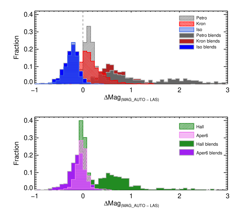
Figure 1.— Comparisons of various total magnitude estimates from the UKIDSS LAS catalog to MAG_AUTO remeasured with SExtractor. UKIDSS Petrosian magnitudes (Petro), Kron magnitudes (Kron), isophotal magnitudes (Iso), Hall magnitudes (Hall), and corrected “total” AperMag6 magnitudes (Aper6) are displayed. Hatched histograms refer to offsets for isolated sources while solid, filled histographs show results for deblended sources.

We begin by demonstrating the amplitude of the UKIDSS total magnitude errors. We have downloaded nearly 6000 UKIDSS image “cutouts” centered on $K$-band bright sources, both isolated and blended and drawn from the s82-mgc, each with a size of $1\arcmin\times 1\arcmin$. We have run SExtractor (Bertin & Arnouts, 1996) on the cutouts and compared its output magnitudes to various total flux estimators in the UKIDSS DR8 catalog. The results are reported in Figure 1. The zeropoint is determined from the keywords stored in the zeroth and first extension headers in each cutout FITS image, following Equation 1 of Hill et al. (2011):

$${\rm ZP}={\rm ZP_{mag}}+2.5\log{t}-{\rm Ext}\times(({\rm AM_{1}}+{\rm AM_{2}})/2-1)$$ (1)

where ${\rm ZP_{mag}}$ refers to the keyword, MAGZPT, $t$ refers to EXP_TIME, ${\rm Ext}$ refers to EXTINCT, and ${\rm AM_{1}}$ and ${\rm AM_{2}}$ refer to AMSTART and AMEND, the beginning and ending airmass values of the exposure. We verify our zeropoint determination by first comparing aperture photometry in the UKIDSS AperMag2 through AperMag6 apertures (corresponding to aperture radii of 1.4, 2, 2.8, 4, and 5.7 arcseconds). Focusing on isolated sources and de-correcting the LAS aperture magnitudes as in Section 3.1, we find that the median LAS photometry is $\sim$0.03 magnitudes brighter in all apertures; we attribute this to small catalog-level corrections discussed in Hodgkin et al. (2009).

Using hatched histograms for isolated sources and solid, filled histograms for blended sources, Figure 1 displays blended total photometry errors in the UKIDSS Petrosian magnitudes (Petro), Kron magnitudes (Kron), Hall magnitudes (Hall), and corrected “total” AperMag6 magnitudes (Aper6). In all cases except for isophotal and AperMag6 magnitudes, LAS catalog photometry of deblended sources is significantly brighter than MAG_AUTO, typically by 0.5–1 magnitude. Petrosian magnitudes provide the poorest estimates, with offsets as large as 3 magnitudes.

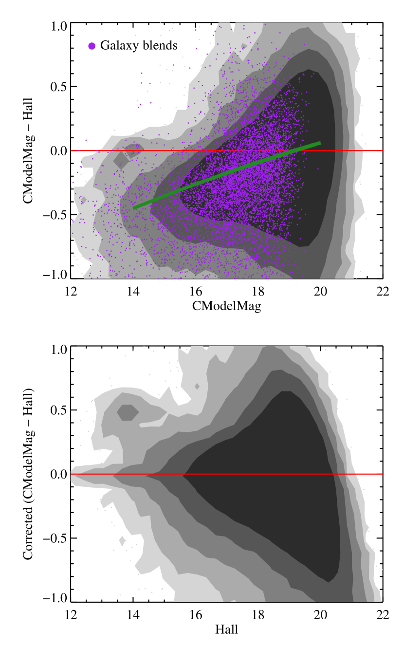
Figure 2.— Illustration of the UKIDSS total magnitude estimator adopted in the s82-mgc. For sources classified as galaxies we plot $K$-band results in this figure, but the other bands are similar. Here CModelMag refers to the UKIDSS aperture magnitude corrected by the difference between the $z$-band synthetic aperture and the $z$-band CModelMag. Blended sources are highlighted in purple and fall off sharply beyond the detection limit ($\sim$19.5). In the top panel, the Hall magnitudes are fainter than CModelMag for bright galaxies. The green curve is a fit to this trend. In the bottom panel, we have corrected the Hall mags of isolated sources using this fit and substituted the CModelMag value for blended sources. This plot of the Hall mag as the dependent variable confirms that there are no biases in the total flux estimator above the detection limit.

For isolated sources, Hall magnitudes correlate best with MAG_AUTO but still suffer biases in the case of blended sources. The “total” magnitudes reported for AperMag6 (i.e., with the UKIDSS aperture correction applied) show the opposite behavior in that blends are fainter than MAG_AUTO on average compared to isolated sources. Even when comparing de-corrected Aper6 magnitudes to the corresponding aperture photometry remeasured by SExtractor, there is a bias such that the reported AperMag6 photometry is 0.05 mag fainter for blends. This bias decreases as the aperture decreases and nearly disappears for Aper4 and smaller apertures. We speculate that the reported aperture magnitudes in the UKIDSS catalog have also been adjusted to remove an estimated contribution from overlapping sources in blended objects, although we could not find UKIDSS documentation to confirm this conclusion. The comparison to “total” AperMag6 values suggests this adjustment introduces a roughly 0.1 magnitude bias towards fainter magnitudes in the large-aperture photometry of blended sources.

The offset for isophotal magnitudes shows no apparent dependence on whether a source is blended. A simple brightening of the reported isophotal photometry by $\sim$0.2 magnitudes brings them into agreement with MAG_AUTO, but the relatively large scatter in the isophotal offset hints at the obvious problem that isophotal magnitudes cannot account for surface brightness dimming and will introduce biases as a function of magnitude (or redshift).

Without a robust total magnitude estimate from UKIDSS for blended sources, we turn to SDSS. Not only does the SDSS Coadd photometry deal with blends, it also fits 2D surface brightness profiles to every source. A recommended total flux estimator is the CModelMag which takes the best linear combination of separate de Vaucouleurs and exponential fits in every SDSS band. Such profile fitting can account for extended surface brightness profiles that cross under the noise background, but, constrained by the profile shape assumptions adopted, they can also introduce biases (e.g., Bernardi et al., 2013).

With these caveats in mind, we build a new total magnitude estimate, HallTot, that is referenced to the UKIDSS Hall magnitudes for non-blended sources and to the SDSS $z$-band CModelMag magnitude for blends. For blends, we apply the offset between the $z$-band synthetic aperture magnitude and CModelMag_z to the aperture magnitude (AperMag4) measured for each UKIDSS band. This choice anchors our UKIDSS total magnitude estimates to CModelMag_z. However, we would prefer to use the UKIDSS Hall mags for isolated sources, given their strong performance with respect to the remeasured MAG_AUTO. The solution is to adjust the Hall mags to also match CModelMag_z on average. The process is illustrated in Figure 2 and delivers blend-resistant HallTot magnitudes for all four UKIDSS bands.

4. Star-Galaxy Separation

Star-galaxy separation in the s82-mgc is more complicated than for typical SDSS imaging data because of problems in the PSF characterization of the Coadd (Annis et al., 2014; Huff et al., 2014). Instead of a classification based on the SDSS TYPE parameter, we use SDSS shape information as a crude first estimate and then refine the classification using the ($J-K$) vs. ($g-i$) colors to separate galaxies (and quasars) from the stellar locus.

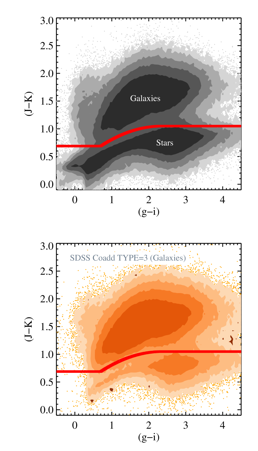
Figure 3.— Top panel: Color-color criteria for star-galaxy separation adopted in the s82-mgc. Shaded contours and data points represent the distribution of sources with $i<21.5$. The colors are Galactic extinction corrected. Bottom panel: Same as above but for SDSS Coadd TYPE$=$3 sources classified as galaxies. The TYPE based galaxy classification is contaminated by a significant fraction ($\sim$10%) of stars, likely as a result of PSF characterization problems in the Coadd. SDSS Coadd point-sources (TYPE$=$6) do not contaminate the color-color based galaxy locus.

Following Baldry et al. (2010) and Strauss et al. (2002), we define the SDSS star-galaxy separation parameter as $\Delta_{\rm sg}=r_{\rm psf}-r_{\rm model}$, where $r_{\rm psf}$ and $r_{\rm model}$ are the $r$-band PSF and ModelMag measurements, respectively. Sources with $\Delta_{\rm sg}>8$ can be confidently classified as (large) galaxies and those with $\Delta_{\rm sg}<0.05$ as point sources. For the remaining sources, we adopt a modified version of the ($J-K$) distance from the stellar locus defined by Baldry et al. (2010):

$$\Delta_{\rm sg,jk}=(J-K)_{\rm AB}-f_{\rm locus}(g-i)$$ (2)

where we correct all colors for Galactic extinction and $f_{\rm locus}(g-i)=-0.523$ for $(g-i)<0.7$, $f_{\rm locus}(g-i)=-0.1632$ for $(g-i)>2.3$. For $0.7<(g-i)<2.3$ the locus is defined as:

$$f_{\rm locus}(g-i)=-0.89+0.615*(g-i)+0.13*(g-i)^{2}$$ (3)

We adopt a color cut defined as $\Delta_{\rm sg,jk}=0.25$ which is displayed in Figure 3.

A check on the completeness and purity of the s82-mgc galaxy classification can be made by comparing to the star-galaxy separator (Leauthaud et al., private communication) based on the overlapping CFHT CS82 $i$-band imaging survey (Kneib et al., in preparation) which delivers excellent shape-based classifications thanks to a median seeing of FWHM$=$0$\farcs$6. First, we note that different internal classifications using CS82 are impure or incomplete at the several percent level, representing a quality floor in typical ground-based data sets. Next, we compare against the “DW” CS82 classification which is based on manual divisions made in the size-magnitude plane. The completeness of the s82-mgc galaxy classification compared to DW is 96%, with a 1% level of contamination from stars. These numbers may be optimistic because both classifiers can fail. A visual inspection of SDSS images suggests that the s82-mgc galaxy sample is contaminated by stars (especially binaries) at the few percent level.

While our classification requires a ($J-K$) color, it performs much better than the Coadd TYPE parameter, used, for example, by Reis et al. (2012) to define a galaxy photo-$z$ sample. As shown in the bottom panel of Figure 3, a Coadd selection with TYPE$=$3 leads to a galaxy sample with at least 10% contamination from the stellar locus.

5. Photometric Redshifts

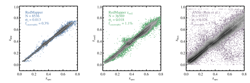
Figure 4.— Comparisons of three photometric redshift estimators to available spectroscopic redshifts in Stripe 82. The comparison is limited to $i<22.5$ and $0.01<z_{\rm spec}<0.8$. The left and middle panels are from the redMaPPer project (Rozo et al., in preparation), while the right panel compares neural-network photo-$z$s from Reis et al. (2012). The 3$\sigma$-clipped dispersion is listed in each panel along with the fraction of catastrophic outliers defined by $\mathinner{\!\left\lvert\Delta z\right\rvert}>0.1$. Contours are plotted at high data densities with 0.3 dex logarithmic spacing in the left and middle panel and 0.4 dex in the right panel. The 1-to-1 relation is plotted in each panel as a thin light grey line.

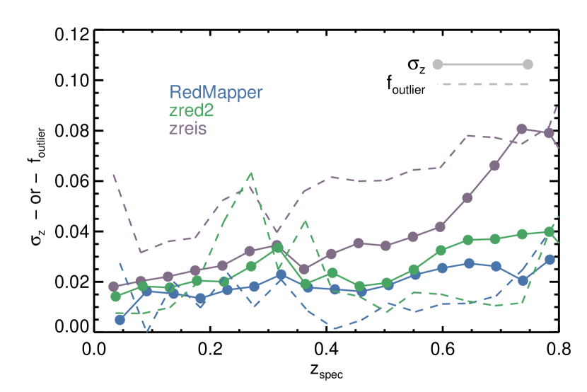
Figure 5.— Photometric redshift-dependent photo-$z$ scatter and outlier fractions for the photo-$z$ estimators used in this paper as compared to available spec-$z$s in Stripe 82 with $i<22.5$ and $0.01<z_{\rm spec}<0.8$. The 3$\sigma$-clipped dispersion ($\sigma_{z}$) is indicated by the solid lines and symbols. The redshift error has not been divided by $(1+z)$. The dashed lines plot $f_{\rm outlier}$, the fraction of photo-$z$s that deviate by more than 3$\sigma$; this is a more stringent definition than $f_{\rm catastrophic}$ sensitive to systematic patterns of scatter that can bias certain redshift bins.

Despite the large number of spectroscopic redshifts in s82-mgc (nearly 73,000 galaxy spec-$z$s, or 11% of galaxies with $i<22.5$), reliable photometric redshifts are paramount for building a complete sample in Stripe 82, given that the majority of the spec-$z$s were obtained from SDSS campaigns employing complex selection criteria.

We have explored a number of photometric redshift estimators and present plots summarizing their performance against available spectroscopic redshifts in Figures 4 and 5. We break with tradition and characterize photo-$z$ scatter without dividing by $(1+z)$ since there is no evidence for such trends in our data. We quote $\sigma_{z}$ as the 3$\sigma$-clipped standard deviation and characterize the outlier fractions with separate parameters. We define catastrophic outliers as those with $\mathinner{\!\left\lvert\Delta z\right\rvert}>0.1$, where $\Delta z$ is difference between the photometric and spectroscopic redshift. Statistical outliers refer to photo-$z$s with $\mathinner{\!\left\lvert\Delta z\right\rvert}$ greater than 3$\sigma_{z}$.

The best photo-$z$ performance for massive galaxies in clusters is produced by the red-sequence Matched-filter Probabilistic Percolation (redMaPPer, Rykoff et al., 2014). For non-cluster galaxies, the best performance is produced by the red-sequence Matched filter Galaxy Catalog (redMaGiC, Rozo et al., 2015) and neural network results derived in Reis et al. (2012) using ANNz (Collister & Lahav, 2004). We use a combination of these estimates to produce the $z_{\rm best}$ redshift estimator appropriate for massive galaxies (see Section 5.3).

We also computed template-based photo-$z$s using BPZ (Benítez, 2000) and EAZY (Brammer et al., 2008) (see Section 5.4). Even after extensive experimentation with various template sets, priors, and zero point offsets, we could not achieve results that were competitive with ANNz (let alone redMaPPer) for bright galaxies. The scatter ($\sigma_{z}$) in photo-$z$–spec-$z$ residuals was typically twice as large with the template codes as compared to ANNz, and the fraction of catastrophic outliers higher by roughly 50%. However, for faint galaxies ($i\gtrsim 22.5$), template codes perform somewhat better, likely because of the smaller training sets available in the face of poorer photometry. We use template photo-$z$s as a check on the neural-network trained redshifts and additionally include them in the s82-mgc with a description below for studies that can benefit from any redshift constraints for the faintest objects in the catalog.

5.1. redMaPPer and redMaGiC photo-$z$s

The best photo-$z$s we have compared—with $\sigma_{z}$ and catastrophic outlier fractions at the 1% level—are those from the recent redMaPPer and redMaGiC catalogs. However, these are limited to red cluster galaxies only (redMaPPer) or red galaxies in general (redMaGiC). As described in detail in Rykoff et al. (2014), redMaPPer’s primary goal is to use the red-sequence method to robustly identify galaxy clusters and their richness using imaging data sets. By training on available spec-$z$s, redMaPPer iteratively defines a model for the redshift dependent red-sequence that can be used to deliver precise photo-$z$s for red galaxies.

We compare redMaPPer and redMaGiC photo-$z$s to available spec-$z$s in the first two panels of Figure 4. redMaPPer photo-$z$s are only available for cluster galaxies, which we define as galaxies in the redMaPPer cluster members catalog that have a minimum membership probability of 90%. For these galaxies, we assign a photometric redshift equal to the photometric redshift of the redMaPPer galaxy cluster. Roughly 4% of s82-mgc galaxies with $i<22.5$ fall in this category. The second estimate we refer to as $z_{\rm red2}$ (or zred2, middle panel of Figure 4). $z_{\rm red2}$ is the starting point for the redMaGiC photometric redshifts. It is the result of applying the empirically derived and redshift-dependent red-sequence template from the cluster finding algorithm to all red galaxies in the sample, regardless of cluster membership. Approximately 20% of s82-mgc galaxies with $i<22.5$ have realizable $z_{\rm red2}$ estimates. Here, we adopt $z_{\rm red2}$ estimates if the quality of the redMaPPer template fit satisfies $\chi^{2}\leq 10$ and the galaxy is brighter than $L_{*}(z)$ luminosity used by the redMaPPer and redMaGiC algorithms. Our criteria for selecting redMaPPer and redMaGiC redshifts were chosen to balance the number of usable photo-$z$s against their quality. More liberal cuts only marginally increase the number of available redMaPPer and redMaGiC photo-$z$s, but significantly decrease their quality.

5.2. ANNz photo-$z$s from Reis et al.

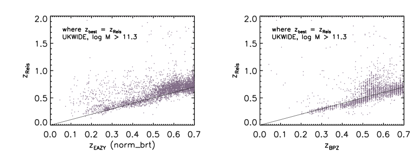
Figure 6.— Independent check of neural network ANNz photo-$z$s, $z_{\rm Reis}$, against EAZY photo-$z$s (left) and BPZ photo-$z$s (right) for a galaxy sample with no other redshift information available (roughly 30% of the ukwide sample across all redshifts). Catastrophic problems in $z_{\rm Reis}$ resulting from inadequate training sets are not evident. Hints of potential photo-$z$ biases at the 0.1 level follow different patterns in the two panels and are difficult to confirm because, by definition, no spec-$z$s are available for this selection.

Reis et al. (2012) compute photo-$z$s using the ANNz neural network code (Collister & Lahav, 2004) applied to $r<24.5$ sources from the SDSS Coadd catalog (Annis et al., 2014) with Coadd TYPE$=$3. As described in Section 4, using this Coadd TYPE criteria to select galaxies results in a sample with $\sim$10% contamination from stars. A more accurate star/galaxy separation is presented in Section 4 and used to define a complete sample, ukwide, in Section 7.

The Reis et al. (2012) photo-$z$s (we refer to them as $z_{\rm Reis}$) were trained and validated with $\sim$83,000 spec-$z$s in Stripe 82. They perform well compared to BOSS galaxies despite having been trained by a more limited spec-$z$ sample that included only 6,682 BOSS redshifts (Figure 4, right-most panel). Comparing to all spec-$z$s now available, we find $\sigma_{z}=0.028$ and a catastrophic outlier fraction of 5.7%, in line with the performance reported in Reis et al. (2012).

While the training set included additional spec-$z$s from deeper surveys, including DEEP2 and VVDS, it is possible that $z_{\rm Reis}$ estimates perform poorly for bright, primarily “blue” galaxies that are not well represented in the training but could be an important contribution to the total massive galaxy population. We test this possibility in Figure 6 by comparing $z_{\rm Reis}$ photo-$z$s to estimates from template codes, $z_{\rm EAZY}$ and $z_{\rm BPZ}$ (see Section 5.4). The comparison is made for sources classified as galaxies in the s82-mgc with $\log{M_{*}/M_{\odot}}>11.3$ and belonging to the ukwide subsample described below (Section 7). We only plot galaxies for which a spec-$z$ or redMaPPer photo-$z$ is not available, thus focusing where our best redshift estimate, $z_{\rm best}$, comes from $z_{\rm Reis}$. About 30% of ukwide galaxies fall in this category at these masses.

Figure 6 demonstrates that there are no catastrophic problems in $z_{\rm Reis}$ resulting from inadequate training sets for massive galaxies with $z<0.7$. While there are hints of potential photo-$z$ biases at the 0.1 level, the patterns of these biases are different when comparing to $z_{\rm EAZY}$ (left panel) or $z_{\rm BPZ}$ (right panel). Given that all three estimators may have biases, it is difficult to say more about biases in $z_{\rm Reis}$ photo-$z$s at this level without additional spec-$z$s.

5.3. Combined photo-$z$s for bright galaxies: $z_{\rm best}$

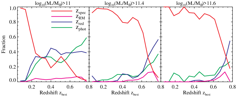
Figure 7.— Fractional contribution of different redshift results as a function of $M_{*}$ and redshift to the “best” estimator, $z_{\rm best}$, appropriate for bright galaxies ($i\lesssim 22.5$) in the s82-mgc. The red line ($z_{\rm spec}$) indicates spec-$z$ from SDSS. The labels $z_{\rm RM}$ and $z_{\rm red}$ refer to redMaPPer. ANNz photo-$z$s from Reis et al. (2012) are labeled $z_{\rm phot}$ and shown in green. See text for details. This figure is reproduced and described further in Paper II.

For bright galaxies ($i\lesssim 22.5$), we combine spec-$z$ and photo-$z$ results together into a single “best” estimate that we refer to as $z_{\rm best}$. In order of priority, $z_{\rm best}$ is set to:

1. $z_{\rm spec}$: Spectroscopic redshifts passing quality cuts from SDSS (including “legacy” and BOSS samples), VVDS, or DEEP2.

2. $z_{\rm RM}$: redMaPPer photo-$z$ for cluster members.

3. $z_{\rm red2}$: redMaGiC photo-$z$ for red field galaxies.

4. $z_{\rm Reis}$: ANNz photo-$z$s from Reis et al. (2012).

The fractional contribution of these estimators as a function of both $M_{*}$ and redshift is shown for the ukwide sample in Figure 7. Paper II studies the SDSS+BOSS spectroscopic completeness evident in this figure. Studies using SDSS+BOSS samples to $z\sim 0.7$ are more than 80% spectroscopically complete at $\log{M_{*}/M_{\odot}}>11.6$ (right-most panel) and only moderately worse at $\log{M_{*}/M_{\odot}}>11.4$ (middle panel).

5.4. Template photo-$z$s for faint galaxies

Template photo-$z$s from EAZY (Brammer et al., 2008) and BPZ (Benítez, 2000) have also been computed to provide a check on $z_{\rm Reis}$ (see above) and additional redshift information for faint sources in the s82-mgc ($i\gtrsim 22.5$). Unlike the Reis et al. (2012) ANNz catalog, we provide template photo-$z$s regardless of star/galaxy classification, in part to enable studies of possibly misclassified compact galaxies, but also to allow future improvements in separating stars and galaxies. As we show, the $z_{\rm Reis}$, $z_{\rm EAZY}$, and $z_{\rm BPZ}$ estimates fail in different ways at the faint end of the s82-mgc sample. One advantage of both EAZY and BPZ is that some control of the failure rate is possible with cuts on the output quality ODDS parameter, if one is willing to limit the usable sample size. These features make the template photo-$z$s useful for source galaxies in weak gravitational lensing studies, for example.

It is well known that template errors in the rest-frame near-IR can lead to degraded photo-$z$ performance when near-IR data is included (e.g., Brammer et al., 2008). Bundy et al. (2012) demonstrated acceptable photo-$z$ performance with near-IR synmags included as a way of validating the synmag methodology. We confirm that the addition of UKIDSS photometry here does not improve the template photo-$z$s, but also does not degrade them when the photometry is appropriately weighted to take template errors into account. In what follows, both $z_{\rm EAZY}$ and $z_{\rm BPZ}$ estimates are therefore based solely on the optical $ugriz$ SDSS Coadd (ModelMag) photometry.

For the $z_{\rm EAZY}$ estimates, we built a custom grid of redshift priors as a function of apparent magnitude via comparisons to the SDSS+BOSS spec-$z$s at bright magnitudes and the complete VVDS spec-$z$s at faint magnitudes. We converted SDSS Coadd inverse hyperbolic sine (asinh) magnitudes (or “luptitudes”, see Lupton et al. 1999) to fluxes and used these as input without any adjustments to the filter band zeropoints. We found the best performance at faint magnitudes using the standard set of EAZY templates. For bright galaxies ($i\sim 20$)—the relevant sample for checking the ANNz $z_{\rm Reis}$ redshifts in Figure 6—we found better results with variants of the Blanton & Roweis (2007) templates (BR07). Aiming to improve outliers in the troublesome $z_{\rm spec}\approx 0.35$ range, we combined results from the EAZY-supplied BR07 template set with a modified version that removed the most extreme star-forming template. We further attempted to calibrate any remaining $z_{\rm EAZY}$ biases and refer to this version of $z_{\rm EAZY}$ estimates as “norm_brt”. Compared to SDSS+BOSS spec-$z$s with no ODDS cut, the norm_brt sample exhibited a $\sigma_{z}$ of 0.03 with an outlier fraction of 18% and a catastrophic outlier fraction of $\sim$10%.

To estimate $z_{\rm BPZ}$, no adjustment to the assumed priors was made, but we did apply the zeropoint offsets that BPZ is able to compute for sources with spec-$z$s. We experimented with several different magnitude cuts when determining these offsets and also tested several SED template sets. These experiments led to only small improvements in photo-$z$ performance.

Given the superior performance of the redMaPPer and ANNz redshifts described above for bright galaxies, we turn now to the quality of $z_{\rm EAZY}$ and $z_{\rm BPZ}$ estimates for the faintest galaxies detected in the s82-mgc. Here $z_{\rm EAZY}$ is derived using the standard EAZY template set. Figure 8 presents comparisons to VVDS and DEEP2 spec-$z$s. VVDS is a magnitude limited survey with $i\lesssim 22.5$, while DEEP2 targets were color-selected to have $z\gtrsim 0.7$ and typically have magnitudes of $i\gtrsim 22.5$ which therefore reach or exceed the s82-mgc detection limits. Catastrophic outliers in the $z_{\rm EAZY}$ estimates tend to congregate near $z_{\rm EAZY}$$\sim 1.1$, likely reflecting the custom priors we have adopted. The $z_{\rm BPZ}$ outliers are more distributed and tend to fall below the true redshift. Particular science cases may prefer one or the other failure mode. In addition, cuts on the ODDS photo-$z$ quality parameter allows cleaner photo-$z$ samples to be obtained (lower panels). For comparison, the $z_{\rm Reis}$ estimates for the DEEP2 sample are shown in Figure 9.

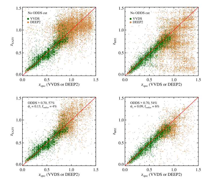
Figure 8.— Photometric redshift quality for the faintest galaxies in the s82-mgc. Results using the template-based EAZY (left panels) and BPZ (right panels) photo-$z$ codes are compared to VVDS and DEEP2 spec-$z$s as indicated. VVDS is a magnitude limited survey with $i\lesssim 22.5$, while DEEP2 targets were color-selected to have $z\gtrsim 0.7$ and typically have magnitudes of $i\gtrsim 22.5$ which therefore reach or exceed the s82-mgc detection limits. Catastrophic outliers display significantly different behavior between the two codes. Given sparse training sets at faint magnitudes, the ODDS parameter output from EAZY and BPZ provides an advantage over neural-network photo-$z$s for selecting better performing photo-$z$ samples. For example, the lower panels show improved results for ODDS$>$0.7. The percentage of the original sample that satisfies the ODDS cut is labeled in each panel as are metrics characterizing the resulting photo-$z$ quality.

Figure 9.— Performance of the $z_{\rm Reis}$ neural-network photo-$z$s when compared to the VVDS and DEEP2 samples used in Figure 8. The $z_{\rm Reis}$ estimates were trained in part on these spec-$z$s but show larger scatter ($\sigma_{z})$ than the template fitting photo-$z$ estimates compared in Figure 8. It is also more difficult to prune high-performing subsets of neural-network estimates.

6. Survey Geometry

A precise measurement of the total valid solid angle over which the s82-mgc sample was drawn is obviously critical to any derivation of source densities. Unfortunately, this measurement is complicated by the relatively large number of intersecting data sets: the Stripe 82 Coadd imaging, the UKIDSS photometry in four separate bands, and the BOSS spectroscopy. Not only must we define the geometric footprint of each data set but also the regions that should be rejected for various reasons, including image artificats and bright stars.

To do so, we have relied heavily on the mangle software package (Swanson et al., 2008) supplemented with both custom built routines and IDL procedures bundled with the SDSS idlutils package. With mangle it is possible to create, manipulate, and determine the intersections and overlap of spherical polygons on the sky. We refer to a set of such polygons as a “mask,” which can represent a survey’s on-sky footprint or a series of “holes” where data should not be considered. Due to the presence of a bug in combining polygon weights in previous mangle versions, we used a development version downloaded in June 2014 from the mangle GitHub repository.

All mangle polygon files in s82-mgc are “pixelized” to a fixed resolution of $r=11$ and “snapped.” We adopt angle tolerances following the DES collaboration (Aurélien Benoit-Lévy, private communication) with cap tolerance variables, “a,” “b,” and “t,” set to 0$\farcs$0027 and the intersection angle tolerance, “m,” set to $10^{-8}$″. From a visual inspection of output polygon masks, we estimate that these mangle settings yield total area estimates that are accurate at the 2% level. A small $\sim$0.8 deg² portion of the final polygon file, with source detections overplotted, is presented in Figure 10.

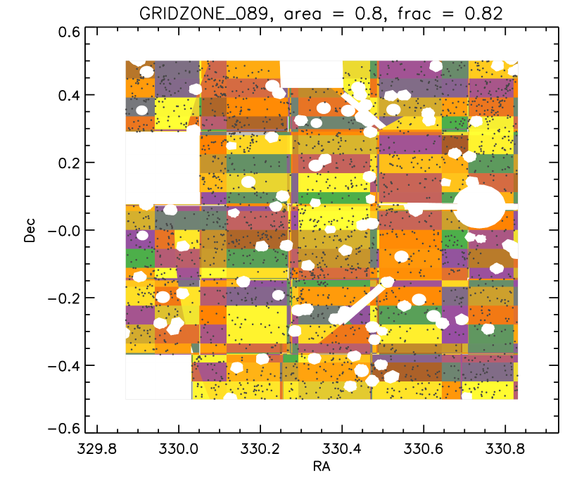
Figure 10.— A small portion of s82-mgc illustrating the union of acceptable survey polygons, each shaded with different colors for visual clarity. White regions correspond to rejection masks for stars, missing data, imaging artifacts, and BOSS targeting limitations. The positions of galaxies from the ukwide subsample (see Section 7) are overplotted.

6.1. BOSS Survey Masks

Because the BOSS team has used mangle tools extensively, several useful masks defining the BOSS survey already exist and are publicly available. We used masks described on the BOSS DR9 Large Scale Structure page on the SDSS-III website. There is little to no difference in the BOSS DR10 masks because no new observations were obtained in Stripe 82 after DR9. Because the BOSS footprint overlaps almost entirely with s82-mgc, applying the BOSS masks when selecting the final s82-mgc sample enables studies of the completeness of BOSS samples (Paper II) and reduces the total area by less than 10%, almost entirely as a result of the BOSS collision priority rejection mask (see Section 6.3).

The BOSS survey footprint (acceptance mask) is defined in the mangle polygon file, boss_geometry_2011_06_10.ply. We also make use of several rejection masks. Beyond the bright star rejection mask, bright_star_mask_pix.ply, the centerpost mask, centerpost_mask.ply, removes a small region associated with the center of each BOSS plate where spectroscopic targets could not be observed. The collision priority mask, collision_priority_mask.ply, accounts for small zones around BOSS galaxy targets that may have been de-prioritized in favor of other source classes (such as quasars). Before application to s82-mgc, all BOSS masks are trimmed to the Stripe 82 region.

6.2. UKIDSS footprint masks

We derive the areal geometry of the four filter bands in the UKIDSS LAS photometry in Stripe 82 using custom software and make the results publicly available on the s82-mgc website. We first define a template for the 4-detector WFCAM imaging footprint following the field layout information on the UKIRT website, and then identify all catalog sources associated with a specific WFCAM multiframe. Multiframes can overlap, miss data from certain detectors, or be truncated, for example from spilling over the edge of the SDSS Coadd region that defined the positional boundaries in the UKDISS catalog query.

For these reasons, we use the catalog source positions to reverse engineer each multiframe’s sky position and determine the geometry of its acceptable imaging. We construct heavily smoothed histograms of the celestial coordinates of associated sources in order to identify the gaps that define the WFCAM footprint. We then adjust the footprint template to match, deriving spherical rectangles that correspond to each detector. Where multiframes are truncated we use this gap information (if a gap exists) and the most extreme source positions to define the maximum extent of each detector. The resulting “framemask” is assigned a “weight” equal to the derived AB magnitude imaging depth discussed in Section 2.2.1 and is converted into the mangle polygon format. The pixelized and snapped UKIDSS footprint masks have file names of the form, mangle_framemask_{y,j,h,k}_v???.ply, where v??? represents a version number.

6.3. Rejection masks

Even in regions with valid UKIDSS or SDSS Coadd photometry, it is important to mask regions around bright stars and associated diffraction spikes, satellite trails, and other image artifacts. Ideally, one would define masks by inspecting actual imaging data, but for wide-field surveys with many bands, this is a challenging data management problem. Instead, we inspect the spatial distribution of cataloged sources across the survey region, distinguishing valid photometric sources from those flagged because of a problem identified by the photometric pipeline. Problematic regions can be identified easily by eye because they exhibit an overdensity of “bad” sources or trace an unphysical geometric pattern (such as a diffraction spike).

We developed a software package that takes a catalog of source positions as input and allows the user to scan through the survey footprint. Bad areas can be traced interactively. The user can draw either a circle by defining the center with one click and the radius with a second, or a generic polygon by clicking a set of points to define the polygon vertices. These shapes are saved, over-plotted, and can be deleted and redrawn. When finished, the software converts the stored shapes into a mangle polygon file that can be used as a rejection mask to define the final survey footprint.

This technique was used to define the rejection masks for all four UKIDSS bands as well as the SDSS Coadd catalog. For each UKIDSS band, the amount of rejected area is $\sim$3 deg². Masking of the SDSS Coadd accounts for 1.2 deg². Most bright stars were already masked by the BOSS bright star rejection mask (4.3 deg² over s82-mgc), but several were missed or were more of a problem in the UKIDSS bands. In the s82-mgc region, the BOSS collision priority mask sums to 16.8 deg² and the centerpost rejection mask amounts to 0.1 deg². The rejection masks are available on the s82-mgc website.

7. The ukwide sample

With the parent SDSS Coadd and UKIDSS data sets defined above, we select a galaxy sample optimized to have a well characterized $M_{*}$ completeness limit as wide an area as possible in the s82-mgc. We refer to this sample as “ukwide.” Forming the basis for the number density evolution and BOSS completeness studies described in Paper II, ukwide contains 517,714 galaxies with matched Coadd+UKIDSS photometry. It covers $139.4$ deg², and is complete above $\log M_{*}/M_{\odot}\approx 11.2$ at $z=0.7$. Data tables corresponding to the ukwide sample are made publicly available as described in the Appendix.

The ukwide sample applies several initial cuts. Galaxies are separated from stars as described in Section 4. We then remove sources located in any of the rejection masks, accounting for bad regions in all four bands of the UKIDSS photometry and the SDSS Coadd imaging, as well as bright stars and zones where BOSS spectroscopy was not possible or incomplete (see Section 6 for more details). We also require the ukwide galaxies to fall in the BOSS DR9 acceptance mask and pass cuts on the UKIDSS ppErrBits error flag.

We must also define the acceptable UKIDSS imaging depths for the ukwide sample. In AB magnitudes, we choose 5$\sigma$ magnitude limits of $[20.32,19.99,19.56,19.41]$ for the four bands, $YJHK$ (see 2.2.1). ukwide contains only those sources drawn from UKIDSS imaging with depths greater than these values. The motivation for these limits is discussed further below.

7.1. $M_{*}$ Completeness Considerations

In constructing the ukwide sample, we have adopted a selection that maximizes the available area with relatively uniform completeness in stellar mass. A conservative estimate for this redshift-dependent $M_{*}$ completeness limit in any filter can be obtained by considering the theoretical range of galaxy stellar mass-to-light ratios ($M_{*}/L$) present at each redshift. If we choose a reasonable representative SED for the maximum $M_{*}/L$ possible (e.g., a stellar population that formed quickly in a burst of star formation at $z\sim 5$) and compare it against the limiting magnitude in the filter band, we can estimate the minimum $M_{*}$ of all galaxies at that redshift with brighter observed magnitudes.

For a reference redshift, we choose $z=0.7$, which roughly corresponds to the redshift limit of the BOSS spectroscopy and the point where the available photometric redshifts become increasingly imprecise. Figure 11 displays the $M_{*}$ limits described above as a function of the magnitude in several bands at this redshift. We focus on the $rizYJHK$ as they provide the most critical constraints on $M_{*}/L$ and $M_{*}$ at these redshifts in the s82-mgc data set. The ideal magnitude limits in each band at some desired $M_{*}$ limit are simply given by the intersection of the plotted lines and that $M_{*}$ limit. The observed $r$-band limit is significantly fainter than the other bands, a result of the 4000Å break at this redshift and the red colors defining the extreme-$M_{*}/L$ SED template.

The SDSS Coadd $riz$ 90% completeness depths are indicated by the solid symbols on the corresponding $riz$ lines. The $r$-band depth limits the completeness of any s82-mgc sample to $\log M_{*}/M_{\odot}\approx 11.1$. The redder bands can afford brighter magnitude limits (in AB units) and still have deeper $M_{*}$ limits at $z=0.7$. By roughly matching the $M_{*}$ limit defined by the $r$-band, we can define ideal magnitude limits (5$\sigma$) for the UKIDSS bands. As shown again by the solid symbols for the $YJHK$ bands, our final adopted limits are indeed close to $\log M_{*}/M_{\odot}\approx 11.1$ at $z=0.7$. In practice, the precise numbers ($[20.32,19.99,19.56,19.41]$ for $YJHK$) were matched to a limit at somewhat lower redshift before testing revealed the fidelity of s82-mgc to redshifts approaching 0.7.

Because the UKIDSS imaging depth is not uniform across Stripe 82, a final consideration for the adopted magnitude limits is the corresponding amount of area available. Working in terms of the $M_{*}$ limit defined at the 5$\sigma$ detection threshold, Figure 12 displays the cumulative distribution of area imaged to depths greater than that limit for each UKIDSS band, again referenced to $z=0.7$. A limit of $\log M_{*}/M_{\odot}\approx 11.1$ at this redshift makes use of all the UKIDSS area available.

We quote the final $M_{*}$ completeness limit for ukwide at $\log M_{*}/M_{\odot}\approx 11.2$. This is a conservative choice that acknowledges potential systematics in the way we estimate the UKIDSS and SDSS Coadd depths, as well as catastrophic errors that may occur in matched photometry and SED fitting when using sources measured at the 5$\sigma$ limit. Effectively, a limit of $\log M_{*}/M_{\odot}\approx 11.2$ corresponds to a brightening of our nominal magnitude limits by 0.25 magnitudes.

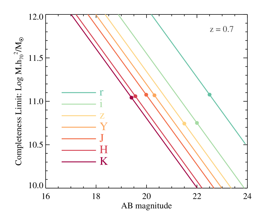
Figure 11.— The estimated $M_{*}$ completeness limit as a function of the limiting depth in relevant s82-mgc filter bands at a specific redshift. Solid symbols indicate the locations of detection limits in each plotted band. The SDSS Coadd $r$-band depth is comparable to the UKIDSS depths in terms of $M_{*}$ completeness.

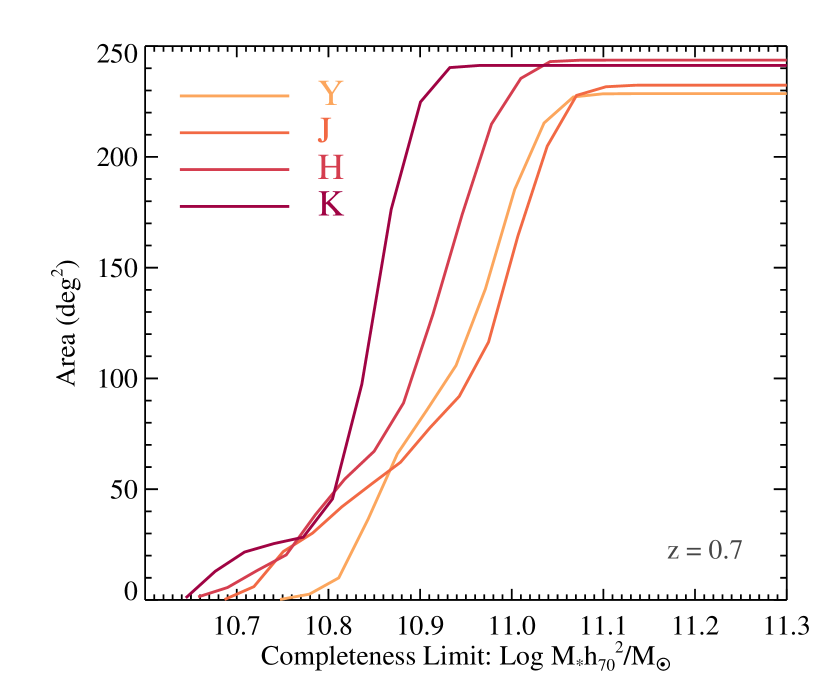
Figure 12.— We plot the area covered in each UKIDSS filter band as a function of the limiting depth expressed in terms of the $M_{*}$ completeness at a specific redshift. Assuming that all other bands are sufficiently deep, the completeness limit corresponds to the faintest theoretical galaxy with a maximum reasonable $M/L$ that is detected at 5$\sigma$ in the relevant band.

8. Derived Galaxy Properties

8.1. The birth parameter, $b_{1000}$

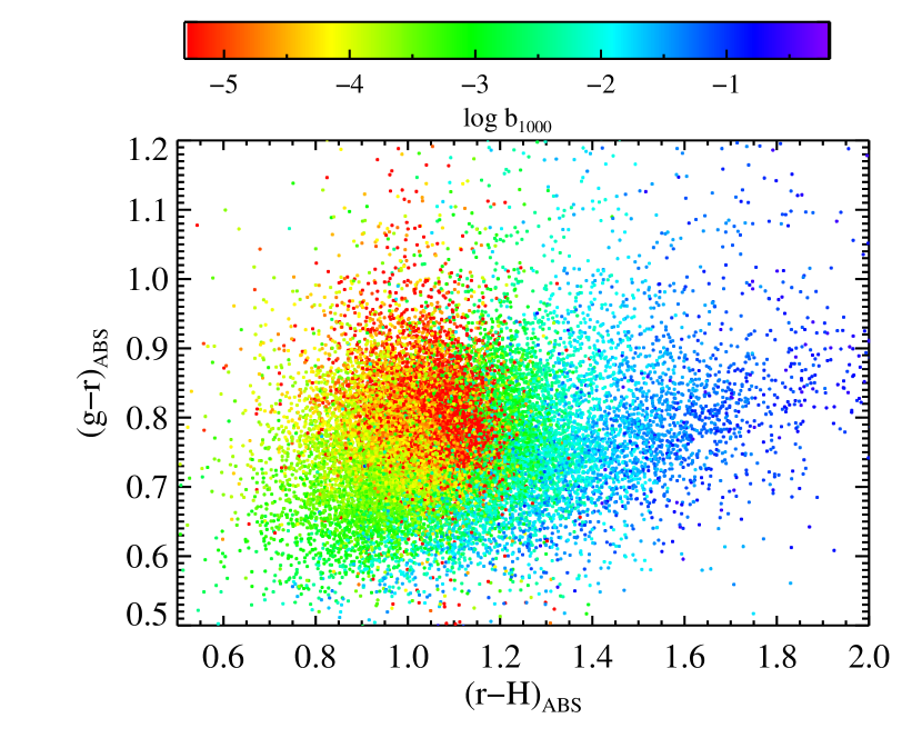
Figure 13.— Correlation between the $b_{1000}$ birth parameter, a proxy for recent star formation, and position in a restframe optical-near-IR color-color diagram for a ukwide sample with $0.3<z_{\rm best}<0.6$ and $\log{M_{*}/M_{\odot}}>11.2$. The value of $\log{b_{1000}}$ is indicated by the associated color, as labeled. The most quiescent galaxies with the lowest $b_{1000}$ parameters (colored red) are clustered at red ($g-r$) colors but relatively blue ($r-H$) colors, as expected (e.g., Williams et al., 2009). Galaxies with more recent star formation (higher $b_{1000}$, bluer colors) span a more extended range in this diagram. Dusty star-formers continue upwards into the optical red sequence, but can be distinguished by their redder ($r-H$) colors.

The presence of recent star formation among galaxies in imaging data sets is often inferred from a rest-frame color that straddles the 4000 Å break. A major benefit of near-IR data is the ability to use color-color diagrams to distinguish red galaxies with underlying but dusty star formation from truly quiescent systems (e.g., Williams et al., 2009). Here we exploit the full optical through near-IR photometry in the s82-mgc to estimate a proxy for recent star formation that accounts for dust. We compress the 2D information in a color-color diagram into a single measurement by fitting the full SEDs available in the s82-mgc with the KCORRECT package (Blanton & Roweis, 2007). KCORRECT provides an estimate of the birth parameter $b_{1000}$, defined as the ratio of the average star formation rate within the previous 1 Gyr to the star formation rate averaged over the galaxy’s history. As with $M_{*}$ estimates, $b_{1000}$ depends on the assumed models and priors used to the fit the observed SEDs. Figure 13 illustrates the correlation between $b_{1000}$ and location in the ($g-r$) versus ($r-H$) diagram. A tight grouping of galaxies with very low $b_{1000}$ values is evident as is a more extended star-forming sequence that includes dusty systems that would otherwise be located on the (optical) red sequence. Visual inspection of the CS82 imaging confirms that these galaxies are predominantly disk-like or disturbed. The use of a near-IR based $b_{1000}$ parameter allows them to be easily distinguished from truly quiescent systems.

In the s82-mgc, galaxies at $z\sim 0.55$ and $M_{*}\sim 11.5$ have $b_{1000}$ values as high as 0.7, suggesting an occasional high rate of recent star formation, but the vast majority are peaked near $b_{1000}=0$ as expected for an old, passively evolving stellar population.

8.2. Stellar Mass Estimates

A key motivation of s82-mgc is providing near-IR photometry for robust $M_{*}$ estimates since the range of possible stellar $M/L$ ratios for stellar populations decreases at near-IR wavelengths. Among the most massive galaxies with $z<1$, the expectation is that the majority have little star formation and are passively evolving. Thus, $M_{*}$ estimates based on optical photometry alone may be sufficient (e.g., Pforr et al., 2012). Still, observed $i$-band corresponds to restframe $g$-band at $z\sim 0.7$, and even the observed $z$-band, which is typically shallower than $r$ or $i$ in single-epoch SDSS imaging, falls blueward of restframe $r$-band. Because young stars significantly bias $M_{*}$ estimates limited to blue restframe wavelengths, the fact that nearly 40% of the CMASS sample is intrinsically associated with the blue cloud (Montero-Dorta et al., 2014) and the evidence for an increase with redshift in the fraction of CMASS galaxies with spectra indicating recent star formation (Chen et al., 2012) motivate restframe near-IR photometry as an important ingredient for checking evolutionary results based on estimates of $M_{*}$.

8.2.1 s82-mgc fiducial $M_{*}$ estimates

The fiducial $M_{*}$ estimates derived for the s82-mgc use the Bayesian code initially presented in Bundy et al. (2006) and used in Bundy et al. (2010). Paper III presents additional mass estimates testing various priors with iSEDfit (Moustakas et al., 2013) based on the s82-mgc photometry for the ukwide sample. The observed SED of each galaxy is compared to a grid of 13,440 models from the Bruzual & Charlot (2003) (BC03) population synthesis code that define a set of priors spanning a (randomized) range of metallicities, star formation histories (parameterized as exponentials), ages, and dust content. Ages are restricted to less than the cosmic age at each redshift and no bursts are included. A Chabrier IMF (Chabrier, 2003), $\Omega_{M}$=0.3, $\Omega_{\Lambda}$=0.7, and a Hubble constant of 70 km s^-1 Mpc^-1 were adopted.

At each grid point, the $M_{*}/L$ ratio in the reddest observed band, the $M_{*}$ value inferred from multiplying $M_{*}/L$ by the luminosity in this band, and the likelihood that the model matches the observed SED are stored. This likelihood is marginalized over the grid, giving an estimate of the stellar mass probability distribution. We take the median as the final estimate of $M_{*}$, which counts the “current” mass in stars and stellar remnants. The 68% width of the distribution provides an uncertainty value which is typically $\sim$0.1 dex.

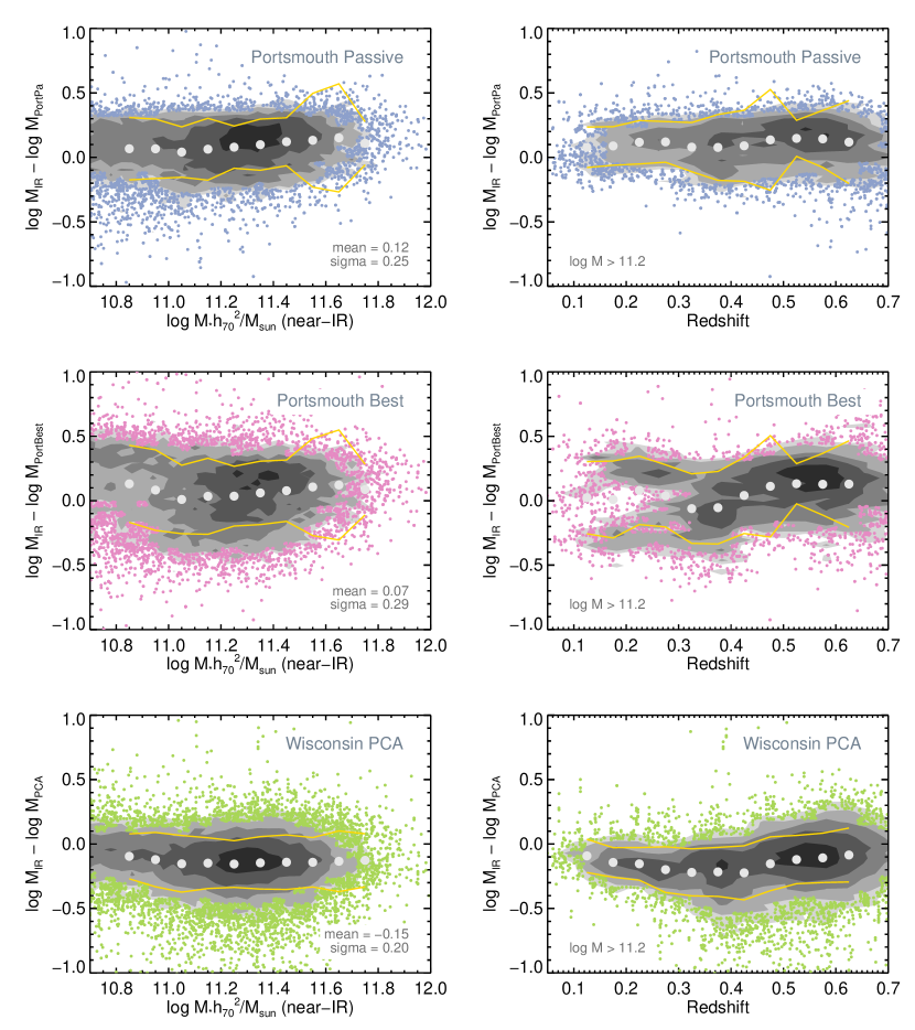
Figure 14.— Comparison of public BOSS $M_{*}$ estimates from Maraston et al. (2013) and Chen et al. (2012) to those presented here (and labeled “near-IR”). Every panel plots the difference in $\log M_{*}$ against near-IR $M_{*}$ in the left column, and against redshift in the right column. The 3$\sigma$-clipped averages (light grey circles) and 1$\sigma$ standard deviation (gold lines) of the difference distributions are over-plotted. Shaded contours with levels separated by 0.3 dex increases in data density are displayed. The comparison is restricted to $\log M_{*}/M_{\odot}>11.2$ for the right-hand panels. Overall normalization differences at the 0.1 dex level are expected. Of greater importance are possible systematic trends that may confuse evolutionary interpretations. Differences in $M_{*}$ estimates display little or no systematic trends with $M_{*}$, but biases, likely resulting from a number of factors, are more apparent as a function of redshift. See text for discussion.

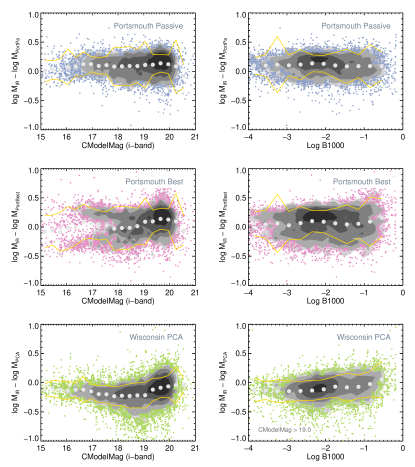
Figure 15.— Mass comparisons as in Figure 14 plotted now as a function of observed magnitude and the $b_{1000}$ parameter, a proxy for the degree of recent star formation less sensitive to dust than an NUV-optical color. Some of the redshift-dependent trends in the $M_{*}$ offsets evident in Figure 14 may result from a more fundamental dependence on magnitude. The comparisons reveal little dependence on $b_{1000}$, despite the fact that the near-IR s82-mgc $M_{*}$ values are less sensitive to biases in $M/L$ owing to recent star formation. The lack of any clear dependence on $b_{1000}$ in the Portsmouth Passive comparison is particularly striking. Galaxies with higher $b_{1000}$ values tend to be at greater redshifts, thus explaining the $b_{1000}$-dependent trend in the Wisconsin comparison.

8.2.2 Extant BOSS $M_{*}$ estimates

Systematic uncertainties are commonly acknowledged in studies employing $M_{*}$ estimates but not always carefully studied. The largest uncertainty is the IMF assumption which, to first order, can cause factor of $\sim$2 offsets in $M_{*}$ values. Setting the IMF aside, Moustakas et al. (2013) provide a careful examination at how different stellar population models and assumptions regarding priors can influence $M_{*}$ estimates based on the same set of photometry. While Moustakas et al. (2013) demonstrate that the conclusions in their paper are largely insensitive to these systematic effects, we adopt a similar methodology in Paper III that reveals the much greater importance of adopted priors and assumptions for constraining massive galaxy evolution with high precision.

This section presents a preview of Paper III by comparing the fiducial near-IR $M_{*}$ estimates described above to publicly available estimates for BOSS galaxies from the SDSS-III collaboration. For a more systematic study of why $M_{*}$ offsets can occur between estimators (including differences in the basis photometry set, stellar synthesis models, and adopted priors), please see Paper III.

In the current work, we only make comparisons to previously (spectroscopically) measured BOSS and SDSS Legacy galaxies that use either the single-epoch SDSS-only photometry or SDSS spectroscopy. We compare this dataset to the “Wisconsin PCA” masses (Chen et al., 2012), two versions of the “Portsmouth” masses described in Maraston et al. (2013, referred to hereafter as M13), and the “Granada” masses released in SDSS DR10 (Ahn et al., 2014). The Granada and Portsmouth masses are based on stellar population synthesis SED fitting to the single-epoch SDSS $ugriz$ ModelMag colors (after correcting for galactic extinction). The Wisconsin PCA masses are derived from a PCA analysis of optical wavelength regions of the BOSS spectra. The resulting $M_{*}/L$ ratios in all three cases are scaled to total magnitudes as given by the CModelMag_i measurements. All BOSS estimates assume a flat cosmology with $\Omega_{m}=0.274$ and $H_{0}=70$ km s^-1 Mpc^-1. The impact on $M_{*}$ from using these cosmological parameters compared to those adopted for the s82-mgc $M_{*}$ estimates is less than 0.01 dex.

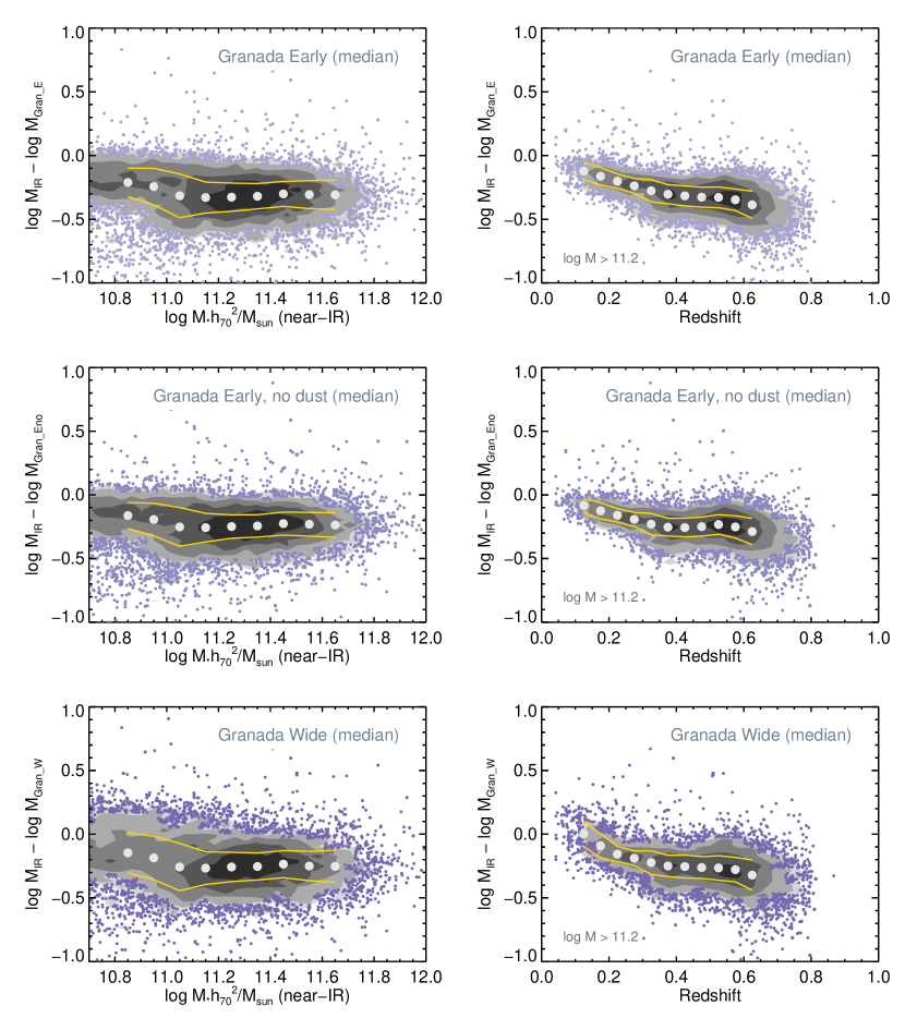
Figure 16.— Mass comparisons, as in Figure 14, to the Granada $M_{*}$ estimates. We consider the median value of the Granada $M_{*}$ posterior distribution. The comparisons show relatively tight scatter but strong redshift-dependent trends that may be induced by a discrepancy in luminosity normalization, as evident in the more uniform trend with observed magnitude presented in Figure 17.

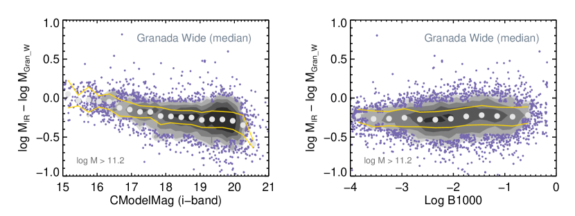
Figure 17.— Granada $M_{*}$ comparisons as a function of observed magnitude and the $b_{1000}$ parameter for the Granada Wide estimates, which are the most similar in adopted priors to the s82-mgc measurements. The relative increase in the Granada $M_{*}$ at faint magnitudes continues smoothly across the full magnitude range, suggesting a difference in luminosity normalization with the s82-mgc estimates.

The “passive” only version of the Portsmouth masses are derived by finding the best fit between the $ugriz$ photometry and a single SED template built from the combination of two passively evolving, coeval bursts of star formation. The first burst is given solar metallicity and accounts for 97% of the total mass, while the second, accounting for the remainder, has 0.05 solar metallicity. Age is the only fitting parameter for this “passive” template but ages less than 3 Gyr are not allowed. A second set of M13 estimates, referred to as “SF”, are based upon fitting stellar population models with a range of star formation histories, ages, and metallicities. Both exponentially declining and truncated star formation histories are included, and an upward correction of +0.25 dex is added based on an analysis of simulated data. Neither of the M13 estimates includes possible dust extinction inside the target galaxy. We use DR10 versions with Kroupa IMFs for the M13 estimates. As with the s82-mgc estimates described in Section 8.2.1, both M13 estimates measure the current mass in stars and stellar remnants at the age of the stellar population model. Maraston et al. (2013) combine the passive and SF estimates into a single, “best” estimate by choosing the passive estimate for galaxies with $(g-i)>2.35$ and the SF estimate for $(g-i)<2.35$. In comparisons described below, we attempt to reproduce the M13 “best” estimates by adopting the passive or SF $M_{*}$ value from the Portsmouth catalogs using the Coadd $(g-i)$ color. There will be slight differences from the actual $M_{*}$ values used in M13 because the Coadd photometry is deeper.

For the Wisconsin PCA masses, Chen et al. (2012) compared their PCA eigenspectra to BC03 models and assume a Kroupa IMF. We only make comparisons for sources with PCA “warning” values set to zero. The PCA mass estimates suffer from aperture biases, which are increasingly important at lower redshifts, and from biases induced by low S/N CMASS spectra which become significant at higher redshifts. Unique to any of the estimates compared here, the Wisconsin masses include priors on the presence of stochastic burst episodes (parameterized by the burst amplitude or mass fraction and a burst duration time) of constant star formation and the possibility of random, abrupt truncations in the star formation history.

The Granada estimates are based on SED fits to the FSPS models (FSPS: Flexible Stellar Population Synthesis Conroy et al., 2009, 2010) and a Bayesian approach similar to that adopted for our fiducial estimates. Four sets of priors are adopted which change the nature of ranges allowed for metallicity, star formation history (parameterized with $\tau$ models), age (less than the cosmic age), and dust content. The “Early” priors restrict to non-star-forming templates. “Wide” priors allow models with more recent star formation. Both of these are available with and without potential dust extinction. We compare our results to Early (with dust), Early (no dust) which is similar to the M13 template, and Wide with dust (which is most similar to our fiducial priors). There are no burst models in the Granada templates. Both median and peak values of the $M_{*}$ posterior are provided. We use the median reported values, but choosing “mean” values does not make a significant difference, although the scatter increases for the “wide” set of priors.

Comparisons of the Portsmouth and PCA masses to our near-IR s82-mgc estimates are shown both as a function of near-IR $M_{*}$ and redshift in Figure 14. Figure 15 presents the same comparisons against observed magnitude and the $b_{1000}$ birth parameter (Section 8.1). A similar set of comparisons against the Granada masses is displayed in Figures 16 and 17.

8.2.3 $M_{*}$ comparison analysis

Despite different prior assumptions compared to the s82-mgc $M_{*}$ estimates and the use of different observational data sets, Figures 14 through 17 demonstrate agreement between the s82-mgc, Portsmouth, Wisconsin, and Granada estimates at the 0.1 dex level, with scatter in the comparisons of 0.2–0.3 dex that is consistent with the expected 0.1–0.2 dex uncertainties associated with any one estimator. As we explore possible trends below, it is important to emphasize that no single estimator can be considered “truth.” The s82-mgc estimates, however, benefit from more precise SEDs (thanks to the deeper Coadd photometry) and, because they are based on the near-IR, are less subject to potential biases from recent star formation. We emphasize that the comparisons discussed here are restricted to bright, BOSS galaxies only. An important advantage of the s82-mgc is the ability to characterize galaxies fainter than BOSS and outside the BOSS selection boundaries in order to build $M_{*}$-complete samples.

In general, overall systematic offsets between $M_{*}$ estimates are tolerable (and expected), but as shown in Paper III, the precision afforded by data sets such as s82-mgc now require understanding subtle dependencies in offsets at the 0.1 dex level. As a function of redshift or galaxy type, systematic biases or changes in the scatter at this level can strongly impact conclusions on evolutionary trends.

Focusing first on the Portsmouth Passive masses, we see a relatively tight relation (upper panels in both figures) against the s82-mgc estimates with a hint of increasing scatter at high $b_{1000}$ values as might be expected if the passive template breaks down for galaxies with more recent star formation. The Portsmouth Best estimates feature more scatter and structure, perhaps revealing how the combination of star-forming templates with a passive template produces a degree of disjoint structure in some regions of parameter space.

The Wisconsin PCA masses feature a tight primary relation with the s82-mgc estimates plus a secondary distribution that scatters downward in the lower panels of Figure 14. Figure 15 (bottom-left panel) suggests this scatter towards larger PCA $M_{*}$ values derives from $i\gtrsim 19$ sources where the BOSS spectral S/N drops and Chen et al. (2012) report biases in their own comparisons to SED-based $M_{*}$ estimates (although the sense of the bias appears to be reversed). A similar bias in the reverse direction was reported in M13. A gentle dependence on $b_{1000}$ (roughly 0.1 dex across the sample) in the Wisconsin comparison is also visible, highlighting the effect of different priors in treating galaxies with more recent star formation (and higher dust extinction). Because the fraction of galaxies with higher $b_{1000}$ values increases with redshift, this trend may underly the redshift dependence in Wisconsin $M_{*}$ offset at $z>0.4$ (Figure 14, bottom-right panel). As the redshift decreases below $z\sim 0.4$, we speculate that aperture effects may drive the Wisconsin masses to lower values compared to the s82-mgc estimates.

Turning now to the Granada masses, Figures 16 and 17 show some of the tightest relations (especially when plotted as a function of redshift, right-hand panels in Figure 16) compared to the s82-mgc estimates. This behavior may not be surprising given the similarity in priors used by Granada compared to the s82-mgc. The level of scatter is comparable to the $z\lesssim 0.4$ regime of the Wisconsin PCA comparison, which is encouraging because the Wisconsin group included bursts and truncated SFHs, but otherwise similar ranges for more continuous SFHs and stellar population parameters.

Despite the tighter scatter, there are strong redshift-dependent trends in the Granada comparisons with $z\sim 0.6$ galaxies about 0.3 dex more massive compared to the s82-mgc estimates than those at $z\sim 0$. This trend flattens somewhat at $z\gtrsim 0.4$, but appears to continue when plotted as a function of observed magnitude (Figure 17, left panel) suggesting a discrepancy in the overall normalization of the luminosity. Understanding this discrepancy will be the subject of future work, but the lack of systematic trends as a function of $M_{*}$ or $b_{1000}$ is nonetheless encouraging.

9. Summary and Conclusions

In this first paper in a series studying massive galaxies in Stripe 82, we have presented a new, publicly available compilation of Stripe 82 data sets, the Stripe 82 Massive Galaxy Catalog (s82-mgc), designed to enable $M_{*}$-limited studies of massive galaxy evolution since $z\sim 0.7$. The catalog includes 9-band $ugrizYJHK$ photometry obtained by matching the SDSS Coadd and UKIDSS-LAS photometric catalogs using the synmag package. Exploiting over 149,439 spectroscopic redshifts, we have assembled and tested a set of photometric redshifts from a variety of sources that are needed to complement spec-$z$s in order to build $M_{*}$ complete samples. With this redshift information, we have derived a new set of near-IR based $M_{*}$ estimates and included them in the s82-mgc.

A number of additional steps have been taken to make the s82-mgc ready for population studies. We have used the near-IR photometry to improve the star-galaxy separation and built new estimates of UKIDSS total magnitudes that address the significant limitations due to blends in the public UKIDSS-LAS catalogs. We have also carefully defined the survey geometry and local depth of the combined data set, designing new custom masks in order to reject problematic regions in both the SDSS Coadd and UKIDSS imaging bands.

Applying these rejection masks and a set of near-IR magnitude limits, we have constructed a $M_{*}$-limited sub-sample of the s82-mgc called ukwide that spans $139.4$ deg² and contains 41,770 galaxies with $\log{M_{*}/M_{\odot}}>11.2$ to $z\approx 0.7$, roughly 45% of which boasts a spectroscopic redshift. This is the largest near-IR selected and $M_{*}$ complete sample of galaxies beyond $z\sim 0.1$ assembled to date. Paper II exploits this sample to study the completeness function in the BOSS samples.

Finally, we have presented comparisons between the near-IR based $M_{*}$ estimates in the s82-mgc and previous, publicly available $M_{*}$ estimates for BOSS galaxies. We analyze various systematic trends that are apparent, and find generally good agreement at the 0.1 dex level. However, as demonstrated in our forthcoming analysis of galaxy $M_{*}$ functions (Paper III), systematics at this level are now a significant limitation in our ability to measure high precision evolution in the massive galaxy population. Encouragingly for the BOSS sample, the addition of near-IR data has only a mild impact on $M_{*}$ estimates, primarily affecting galaxies with more recent star formation.

10. Acknowledgments

This work was supported by World Premier International Research Center Initiative (WPI Initiative), MEXT, Japan. This work was supported by a Kakenhi Grant-in-Aid for Scientific Research 24740119 from Japan society for the Promotion of Science. We thank E. Rykoff and E. Rozo for a generous contribution of redMaPPer photometric redshift estimates. This publication has made use of code written by James R. A. Davenport. We are grateful to Aurélien Benoit-Lévy for help with setting mangle parameters.

Funding for SDSS-III has been provided by the Alfred P. Sloan Foundation, the Participating Institutions, the National Science Foundation, and the U.S. Department of Energy Office of Science. The SDSS-III web site is http://www.sdss3.org/.

SDSS-III is managed by the Astrophysical Research Consortium for the Participating Institutions of the SDSS-III Collaboration including the University of Arizona, the Brazilian Participation Group, Brookhaven National Laboratory, Carnegie Mellon University, University of Florida, the French Participation Group, the German Participation Group, Harvard University, the Instituto de Astrofisica de Canarias, the Michigan State/Notre Dame/JINA Participation Group, Johns Hopkins University, Lawrence Berkeley National Laboratory, Max Planck Institute for Astrophysics, Max Planck Institute for Extraterrestrial Physics, New Mexico State University, New York University, Ohio State University, Pennsylvania State University, University of Portsmouth, Princeton University, the Spanish Participation Group, University of Tokyo, University of Utah, Vanderbilt University, University of Virginia, University of Washington, and Yale University.

Appendix A UKIDSS Query

⬇

SELECT s.sourceID, s.RA, s.dec, s.mergedClassStat, s.mergedClass,

s.pStar, s.pGalaxy, s.pNoise, s.pSaturated, s.eBV, s.aY, s.aJ, s.aH, s.aK,

s.yPetroMag, s.yPetroMagErr, s.yHallMag, s.yHallMagErr, ydtcn.IsoMag AS YIsoMag, s.yppErrBits,

s.yAperMag3, s.yAperMag3Err, s.yAperMag4, s.yAperMag4Err, s.yAperMag6, s.yAperMag6Err,

ymd.aperCor3 AS yaperCor3, ymd.aperCor4 AS yaperCor4, ymd.aperCor6 AS yaperCor6,

ymd.seeing AS yseeing, ymd.skyCorrCat as ySkyCorrCat,

ymd.photZPCat as yPhotZPCat, ymd.photZPErrCat as yPhotZPErrCat,

ydtcn.aperMag1 AS yaperMag1, ydtcn.AperMag1Err AS yAperMag1Err, ymd.aperCor1 as yaperCor1,

ydtcn.aperMag2 AS yaperMag2, ydtcn.AperMag2Err AS yAperMag2Err, ymd.aperCor2 as yaperCor2,

ydtcn.aperMag5 AS yaperMag5, ydtcn.AperMag5Err AS yAperMag5Err, ymd.aperCor5 as yaperCor5,

ydtcn.ell AS yEll, ydtcn.pHeight AS ypHeight, ydtcn.pHeightErr AS ypHeightErr,

s.j_1PetroMag, s.j_1PetroMagErr, s.j_1HallMag, s.j_1HallMagErr, j_1dtcn.IsoMag AS J_1IsoMag,

s.j_1ppErrBits,

s.j_1AperMag3, s.j_1AperMag3Err, s.j_1AperMag4, s.j_1AperMag4Err, s.j_1AperMag6, s.j_1AperMag6Err,

j_1md.aperCor3 AS j_1aperCor3, j_1md.aperCor4 AS j_1aperCor4, j_1md.aperCor6 AS j_1aperCor6,

j_1md.seeing AS j_1seeing, j_1md.skyCorrCat as j_1SkyCorrCat,

j_1md.photZPCat as j_1PhotZPCat, j_1md.photZPErrCat as j_1PhotZPErrCat,

j_1dtcn.aperMag1 AS j_1aperMag1, j_1dtcn.AperMag1Err AS j_1AperMag1Err, j_1md.aperCor1 as j_1aperCor1,

j_1dtcn.aperMag2 AS j_1aperMag2, j_1dtcn.AperMag2Err AS j_1AperMag2Err, j_1md.aperCor2 as j_1aperCor2,

j_1dtcn.aperMag5 AS j_1aperMag5, j_1dtcn.AperMag5Err AS j_1AperMag5Err, j_1md.aperCor5 as j_1aperCor5,

j_1dtcn.ell AS j_1Ell, j_1dtcn.pHeight AS j_1pHeight, j_1dtcn.pHeightErr AS j_1pHeightErr,

s.hPetroMag, s.hPetroMagErr, s.hHallMag, s.hHallMagErr, hdtcn.IsoMag AS HIsoMag, s.hppErrBits,

s.hAperMag3, s.hAperMag3Err, s.hAperMag4, s.hAperMag4Err, s.hAperMag6, s.hAperMag6Err,

hmd.aperCor3 AS haperCor3, hmd.aperCor4 AS haperCor4, hmd.aperCor6 AS haperCor6,

hmd.seeing AS hseeing, hmd.skyCorrCat as hSkyCorrCat,

hmd.photZPCat as hPhotZPCat, hmd.photZPErrCat as hPhotZPErrCat,

hdtcn.aperMag1 AS haperMag1, hdtcn.AperMag1Err AS hAperMag1Err, hmd.aperCor1 as haperCor1,

hdtcn.aperMag2 AS haperMag2, hdtcn.AperMag2Err AS hAperMag2Err, hmd.aperCor2 as haperCor2,

hdtcn.aperMag5 AS haperMag5, hdtcn.AperMag5Err AS hAperMag5Err, hmd.aperCor5 as haperCor5,

hdtcn.ell AS hEll, hdtcn.pHeight AS hpHeight, hdtcn.pHeightErr AS hpHeightErr,

s.kPetroMag, s.kPetroMagErr, s.kHallMag, s.kHallMagErr, kdtcn.IsoMag AS KIsoMag, s.kppErrBits,

s.kAperMag3, s.kAperMag3Err, s.kAperMag4, s.kAperMag4Err, s.kAperMag6, s.kAperMag6Err,

kmd.aperCor3 AS kaperCor3, kmd.aperCor4 AS kaperCor4, kmd.aperCor6 AS kaperCor6,

kmd.seeing AS kseeing, kmd.skyCorrCat as kSkyCorrCat,

kmd.photZPCat as kPhotZPCat, kmd.photZPErrCat as kPhotZPErrCat,

kdtcn.aperMag1 AS kaperMag1, kdtcn.AperMag1Err AS kAperMag1Err, kmd.aperCor1 as kaperCor1,

kdtcn.aperMag2 AS kaperMag2, kdtcn.AperMag2Err AS kAperMag2Err, kmd.aperCor2 as kaperCor2,

kdtcn.aperMag5 AS kaperMag5, kdtcn.AperMag5Err AS kAperMag5Err, kmd.aperCor5 as kaperCor5,

kdtcn.ell AS kEll, kdtcn.pHeight AS kpHeight, kdtcn.pHeightErr AS kpHeightErr,

l.ymfID as ymfID, l.yeNum as yeNum, l.j_1mfID as j_1mfID, l.j_1eNum as j_1eNum, l.j_2mfID as j_2mfID,

l.j_2eNum as j_2eNum, l.hmfID as hmfID, l.heNum as heNum, l.kmfID as kmfID, l.keNum as keNum

FROM

lasSource AS s, lasMergeLog AS l,

MultiframeDetector AS ymd, MultiframeDetector AS j_1md, MultiframeDetector AS j_2md,

MultiframeDetector AS hmd, MultiframeDetector AS kmd,

lasDetection AS ydtcn, lasDetection AS j_1dtcn, lasDetection AS j_2dtcn,

lasDetection AS hdtcn, lasDetection AS kdtcn

WHERE

s.frameSetID = l.frameSetID AND

l.ymfID = ymd.multiframeID AND

l.yeNum = ymd.extNum AND

l.j_1mfID = j_1md.multiframeID AND

l.j_1eNum = j_1md.extNum AND

l.j_2mfID = j_2md.multiframeID AND

l.j_2eNum = j_2md.extNum AND

l.hmfID = hmd.multiframeID AND

l.heNum = hmd.extNum AND

l.kmfID = kmd.multiframeID AND

l.keNum = kmd.extNum AND

l.ymfID = ydtcn.multiframeID AND

l.yeNum = ydtcn.extNum AND

s.ySeqNum = ydtcn.SeqNum AND

l.j_1mfID = j_1dtcn.multiframeID AND

l.j_1eNum = j_1dtcn.extNum AND

s.j_1SeqNum = j_1dtcn.SeqNum AND

l.j_2mfID = j_2dtcn.multiframeID AND

l.j_2eNum = j_2dtcn.extNum AND

s.j_2SeqNum = j_2dtcn.SeqNum AND

l.hmfID = hdtcn.multiframeID AND

l.heNum = hdtcn.extNum AND

s.hSeqNum = hdtcn.SeqNum AND

l.kmfID = kdtcn.multiframeID AND

l.keNum = kdtcn.extNum AND

s.kSeqNum = kdtcn.SeqNum AND

(s.priOrSec <= 0 OR s.priOrSec = s.frameSetID) AND

s.dec > -1.3 AND s.dec < 1.3 AND (s.ra between 0 AND 30)

Appendix B s82-mgc Data Products

Several types of s82-mgc data products are made publicly available at s82mgc.massivegalaxies.com. Documentation on the website provides the most up-to-date description of these products. We summarize what is available below. In some cases to make file sizes more manageable, we have divided Stripe 82 into east and west sections by splitting at $\alpha_{\rm J2000}=0$.

Parent Catalogs

Parent photometric catalogs in FITS table format for the east and west side of Stripe 82 are provided from queries of the SDSS Coadd and UKIDSS LAS databases. The Coadd parent catalogs have filenames beginning with “S82coadd_” and contain the Coadd photometry and SDSS profile fitting results. The UKIDSS catalogs have filenames beginning with “las_DR8_” and contain the UKIDSS photometry, error flags, seeing, aperture corrections, and other information from the UKIDSS LAS database.

The Stripe 82 Massive Galaxy Catalog

The heart of the s82-mgc itself, with a filename starting with “pcatd_”, is selected on the SDSS Coadd parent catalog to include Coadd sources with measured $r$-band profile fit information (in practice sources with devAB_R and ExpAB_R $>$ 0.01 are selected). The pcat table includes cross-referencing information for the UKIDSS catalog, matched SDSS+UKIDSS synmag photometry, and corrected UKIDSS total magnitudes, among other selected information from both parent catalogs. The pcat FITS table is a single file that contains 15,342,585 with 92 tags for a total size of 5.5 GB.

Galaxy Properties

Additional FITS tables, matched one-to-one to the pcat, provide estimates of galaxy properties for sources in the s82-mgc. These include spectroscopic redshifts from SDSS, VVDS, and DEEP2 and all photometric redshifts discussed in Section 5. The s82-mgc fiducial $M_{*}$ estimates as well as KCORRECT absolute magnitudes and $b_{1000}$ values are also provided. Please see the website for details.

The ukwide sample

For those interested in working with the $M_{*}$-limited ukwide galaxy sample, smaller sub-catalogs of the pcat and galaxy property tables are provided. Some software tools needed to construct ukwide, e.g., the star-galaxy separation, are also included.

Survey Footprint

The UKIDSS depth information and all mangle polygon files describing the geometric layout of the different survey components as well as the rejection masks are provided and described on the website.

References

- Abazajian et al. (2009) Abazajian, K. N. et al. 2009, ApJS, 182, 543
- Ahn et al. (2014) Ahn, C. P., Alexandroff, R., Allende Prieto, C., Anders, F., Anderson, S. F., Anderton, T., Andrews, B. H., Aubourg, É., Bailey, S., Bastien, F. A., & et al. 2014, ApJS, 211, 17
- Aihara et al. (2011) Aihara, H. et al. 2011, ApJS, 193, 29
- Annis et al. (2014) Annis, J. et al. 2014, ApJ, 794, 120
- Baldry et al. (2010) Baldry, I. K. et al. 2010, MNRAS, 404, 86
- Benítez (2000) Benítez, N. 2000, ApJ, 536, 571
- Bernardi et al. (2013) Bernardi, M., Meert, A., Sheth, R. K., Vikram, V., Huertas-Company, M., Mei, S., & Shankar, F. 2013, MNRAS, 436, 697
- Bertin & Arnouts (1996) Bertin, E. & Arnouts, S. 1996, A&AS, 117, 393
- Blanton & Roweis (2007) Blanton, M. R. & Roweis, S. 2007, AJ, 133, 734
- Bolton et al. (2012) Bolton, A. S. et al. 2012, AJ, 144, 144
- Brammer et al. (2008) Brammer, G. B., van Dokkum, P. G., & Coppi, P. 2008, ApJ, 686, 1503
- Bruzual & Charlot (2003) Bruzual, G. & Charlot, S. 2003, MNRAS, 344, 1000
- Bundy et al. (2012) Bundy, K., Hogg, D. W., Higgs, T. D., Nichol, R. C., Yasuda, N., Masters, K. L., Lang, D., & Wake, D. A. 2012, AJ, 144, 188
- Bundy et al. (2006) Bundy, K. et al. 2006, ApJ, 651, 120
- Bundy et al. (2010) —. 2010, ApJ, 719, 1969
- Capak et al. (2007) Capak, P. et al. 2007, ApJS, 172, 99
- Chabrier (2003) Chabrier, G. 2003, PASP, 115, 763
- Chen et al. (2012) Chen, Y.-M. et al. 2012, MNRAS, 421, 314
- Coil et al. (2011) Coil, A. L., Blanton, M. R., Burles, S. M., Cool, R. J., Eisenstein, D. J., Moustakas, J., Wong, K. C., Zhu, G., Aird, J., Bernstein, R. A., Bolton, A. S., & Hogg, D. W. 2011, ApJ, 741, 8
- Collister & Lahav (2004) Collister, A. A. & Lahav, O. 2004, PASP, 116, 345
- Conroy et al. (2009) Conroy, C., Gunn, J. E., & White, M. 2009, ApJ, 699, 486
- Conroy et al. (2010) Conroy, C., White, M., & Gunn, J. E. 2010, ApJ, 708, 58
- Davis et al. (2003) Davis, M. et al. 2003, in SPIE, Vol. 4834, 161–172
- Dawson et al. (2013) Dawson, K. S. et al. 2013, AJ, 145, 10
- Drinkwater et al. (2010) Drinkwater, M. J., Jurek, R. J., Blake, C., Woods, D., Pimbblet, K. A., Glazebrook, K., Sharp, R., Pracy, M. B., Brough, S., Colless, M., Couch, W. J., Croom, S. M., Davis, T. M., Forbes, D., Forster, K., Gilbank, D. G., Gladders, M., Jelliffe, B., Jones, N., Li, I.-H., Madore, B., Martin, D. C., Poole, G. B., Small, T., Wisnioski, E., Wyder, T., & Yee, H. K. C. 2010, MNRAS, 401, 1429
- Eisenstein et al. (2001) Eisenstein, D. J. et al. 2001, AJ, 122, 2267
- Eisenstein et al. (2011) —. 2011, AJ, 142, 72
- Frieman et al. (2008) Frieman, J. A. et al. 2008, AJ, 135, 338
- Fukugita et al. (1996) Fukugita, M., Ichikawa, T., Gunn, J. E., Doi, M., Shimasaku, K., & Schneider, D. P. 1996, AJ, 111, 1748
- Gunn et al. (1998) Gunn, J. E. et al. 1998, AJ, 116, 3040
- Gunn et al. (2006) —. 2006, AJ, 131, 2332
- Hall & Mackay (1984) Hall, P. & Mackay, C. D. 1984, MNRAS, 210, 979
- Hewett et al. (2006) Hewett, P. C., Warren, S. J., Leggett, S. K., & Hodgkin, S. T. 2006, MNRAS, 367, 454
- Heymans et al. (2012) Heymans, C. et al. 2012, MNRAS, 427, 146
- Hildebrandt et al. (2012) Hildebrandt, H. et al. 2012, MNRAS, 421, 2355
- Hill et al. (2011) Hill, D. T. et al. 2011, MNRAS, 412, 765
- Hodgkin et al. (2009) Hodgkin, S. T., Irwin, M. J., Hewett, P. C., & Warren, S. J. 2009, MNRAS, 394, 675
- Hogg & Lang (2013) Hogg, D. W. & Lang, D. 2013, PASP, 125, 719
- Huff et al. (2014) Huff, E. M., Hirata, C. M., Mandelbaum, R., Schlegel, D., Seljak, U., & Lupton, R. H. 2014, MNRAS, 440, 1296
- Jiang et al. (2014) Jiang, L., Fan, X., Bian, F., McGreer, I. D., Strauss, M. A., Annis, J., Buck, Z., Green, R., Hodge, J. A., Myers, A. D., Rafiee, A., & Richards, G. 2014, ApJS, 213, 12
- Kron (1980) Kron, R. G. 1980, ApJS, 43, 305
- Lang et al. (2014) Lang, D., Hogg, D. W., & Schlegel, D. J. 2014, ArXiv e-prints
- Lawrence et al. (2007) Lawrence, A. et al. 2007, MNRAS, 379, 1599
- Le Fèvre et al. (2005) Le Fèvre, O. et al. 2005, A&A, 439, 845
- Leauthaud et al. (2015) Leauthaud, A., Bundy, K., Saito, S., Tinker, J., Maraston, C., Tojeiro, R., Huang, S., Brownstein, J. R., Schneider, D. P., & Thomas, D. 2015, ArXiv e-prints
- Lupton et al. (1999) Lupton, R. H., Gunn, J. E., & Szalay, A. S. 1999, AJ, 118, 1406
- Lupton et al. (2002) Lupton, R. H., Ivezic, Z., Gunn, J. E., Knapp, G., Strauss, M. A., & Yasuda, N. 2002, in Society of Photo-Optical Instrumentation Engineers (SPIE) Conference Series, Vol. 4836, Survey and Other Telescope Technologies and Discoveries, ed. J. A. Tyson & S. Wolff, 350–356
- Maraston et al. (2013) Maraston, C. et al. 2013, MNRAS, 435, 2764
- Matsuoka & Kawara (2010) Matsuoka, Y. & Kawara, K. 2010, MNRAS, 405, 100
- Montero-Dorta et al. (2014) Montero-Dorta, A. D., Bolton, A. S., Brownstein, J. R., Swanson, M., Dawson, K., Prada, F., Eisenstein, D., Maraston, C., Thomas, D., Comparat, J., Chuang, C.-H., McBride, C. K., Favole, G., Guo, H., Rodriguez, S., & Schneider, D. P. 2014, ArXiv e-prints
- Moustakas et al. (2013) Moustakas, J., Coil, A., Aird, J., Blanton, M. R., Cool, R. J., Eisenstein, D. J., Mendez, A. J., Wong, K. C., Zhu, G., & Arnouts, S. 2013, ArXiv e-prints
- Newman et al. (2013) Newman, J. A. et al. 2013, ApJS, 208, 5
- Oke & Gunn (1983) Oke, J. B. & Gunn, J. E. 1983, ApJ, 266, 713
- Petrosian (1976) Petrosian, V. 1976, ApJ, 209, L1
- Pforr et al. (2012) Pforr, J., Maraston, C., & Tonini, C. 2012, MNRAS, 422, 3285
- Reis et al. (2012) Reis, R. R. R., Soares-Santos, M., Annis, J., Dodelson, S., Hao, J., Johnston, D., Kubo, J., Lin, H., Seo, H.-J., & Simet, M. 2012, ApJ, 747, 59
- Rozo et al. (2015) Rozo, E. et al. 2015, ArXiv e-prints
- Rykoff et al. (2014) Rykoff, E. S. et al. 2014, ApJ, 785, 104
- Saito et al. (2015) Saito, S., Leauthaud, A., Hearin, A. P., Bundy, K., Zentner, A. R., Behroozi, P. S., Reid, B. A., Sinha, M., Coupon, J., Tinker, J. L., White, M., & Schneider, D. P. 2015, ArXiv e-prints
- Smee et al. (2012) Smee, S. et al. 2012, ArXiv e-prints
- Strauss et al. (2002) Strauss, M. A. et al. 2002, AJ, 124, 1810
- Swanson et al. (2008) Swanson, M. E. C., Tegmark, M., Hamilton, A. J. S., & Hill, J. C. 2008, MNRAS, 387, 1391
- Williams et al. (2009) Williams, R. J., Quadri, R. F., Franx, M., van Dokkum, P., & Labbé, I. 2009, ApJ, 691, 1879
- Wright et al. (2010) Wright, E. L. et al. 2010, AJ, 140, 1868
- York et al. (2000) York, D. G. et al. 2000, AJ, 120, 1579