Modeling Long-term Outcomes and Treatment Effects After Androgen Deprivation Therapy for Prostate Cancer
Abstract
Analyzing outcomes in long-term cancer survivor studies can be complex. The effects of predictors on the failure process may be difficult to assess over longer periods of time, as the commonly used assumption of proportionality of hazards holding over an extended period is often questionable. In this manuscript, we compare seven different survival models that estimate the hazard rate and the effects of proportional and non-proportional covariates. In particular, we focus on an extension of the the multi-resolution hazard (MRH) estimator, combining a non-proportional hierarchical MRH approach with a data-driven pruning algorithm that allows for computational efficiency and produces robust estimates even in times of few observed failures. Using data from a large-scale randomized prostate cancer clinical trial, we examine patterns of biochemical failure and estimate the time-varying effects of androgen deprivation therapy treatment and other covariates. We compare the impact of different modeling strategies and smoothness assumptions on the estimated treatment effect. Our results show that the benefits of treatment diminish over time, possibly with implications for future treatment protocols.
Key Words: biochemical failure, MRH, multi-resolution hazard, non-proportional hazards, prostate cancer, survival analysis.
1 Introduction
Many human cancers today are considered “chronic diseases”, with long-term disease trajectories and multiple co-morbidities. Consequently, long-term cancer outcomes may be affected by numerous factors, ranging from obvious patient and treatment characteristics to secular and health care trends that affect treatment policy and practice. However, the long-term nature of patient and health-care related processes and changing complexity of information can make the analysis of long-term patterns in cancer survivor data sets challenging. In addition to sparsely observed failure times, these data often exhibit non-proportional effects over time, requiring flexible and computationally efficient statistical methods to characterize the evolving failure hazard.
The motivating problem in this article comes from a set of prostate cancer clinical trials from the Radiation Therapy Oncology Group (RTOG), which are specifically designed to examine the effects of the length of androgen deprivation (AD) therapy on disease-free and overall survival time. As a result of the insight gained from these studies over the years, the short-term benefits of AD therapy have been well-understood to delay the time until prostate cancer recurrence and until death (Pilepich et al., 2001, 2005). In addition, longer-duration AD therapy has proven more beneficial than a shorter-duration therapy (Horwitz et al., 2008). However, given that AD treatments can have unpleasant side-effects, clinicians have been reluctant to assign androgen deprivation for longer than necessary.
Many questions remain regarding the relationship between the length of AD therapy and long-term outcomes, such as eventual time to recurrence (Schröder et al., 2012). These open questions still exist in part because prostate cancer is generally a slow cancer to progress (Albertsen et al., 2005). While prostate cancer patients tend to survive longer and are thus observed over extended periods of time, treatment benefits have been difficult to precisely ascertain due to a multitude of co-morbidities and sparsity of information at long follow-up times.
Thus, assessing the long-term benefits of different duration of AD therapy for patients in different risk classes would be of great value to clinical practice and management of prostate cancer patients in general (Schröder et al., 2012). Gaining insight into recurrence patterns and quantifying the degree and length of long-term benefits over time would greatly improve the quality of life for men with this disease. For this reason, the focus of our paper goes beyond integrated summaries such as survival curves and cumulative incidence functions, and concentrates on estimation and inference about the time-dynamic hazard function in the presence of covariates, and the time-evolving predictive probabilities of disease recurrence.
The underlying statistical approach employed in this paper is an extension of the multi-resolution hazard (MRH) model, a Bayesian semi-parametric hazard rate estimator previously presented and used in Bouman et al. (2005, 2007), Dukic and Dignam (2007), Dignam et al. (2009), Chen et al. (2014), and Hagar et al. (2014a). This flexible class of models for time-to-event data is based on the Polya tree methodology, and is also similar in spirit to the adaptive piece-wise constant exponential models (Ibrahim et al., 2001). The MRH parametrization is designed for multi-resolution inference capable of accommodating periods of sparse events and varying smoothness, typical in long-term studies. In addition, the MRH model accommodates both proportional and non-proportional effects of predictors over time. The current methodology employs the pruning algorithm presented in Chen et al. (2014), which performs adaptive and data-driven “pre-smoothing” of the hazard rate, via merging of time intervals with similar hazard levels. Pruning has been shown to increase computational efficiency and reduce overall uncertainty in hazard rate estimation in the presence of periods with smooth hazard rate and low event counts (Chen et al., 2014). All MRH models have been fitted using the ‘MRH” R package (Hagar et al., 2014b).
This paper is organized as follows. In the next section, we provide a short overview of the prostate cancer clinical trials data, and the statistical issues related to these studies with long-term follow-up. Sections 3 and 4 present the corresponding MRH methodology and implementation. Section 5 presents the analysis of biochemical failure in prostate cancer, with comparisons of the MRH approach to a set of alternative models: the Cox proportional hazards model, an extended Cox model that includes a time-varying treatment effect, a non-proportional hazards Weibull parametric model, a semi-parametric Bayesian accelerated failure time model, a dependent Dirichlet Process survival model, and two piece-wise exponential models. In addition we perform a sensitivity analysis to the priors in the MRH model. The article concludes with a discussion of the clinical and statistical importance and implications of our findings.
2 Motivating Example: Androgen Deprivation in Prostate Cancer
Typical prostate treatment involves radiation therapy combined with some form and duration of hormone treatment, which is known as androgen deprivation (AD) therapy. The motivation for the current analysis is the characterization of the hazard rate of time-to-biochemical failure, adjusted for the (potentially) time-varying effects of AD therapy and several key covariates, as described below.
The outcome of interest in this analysis, “biochemical failure”, is defined according to the Phoenix definition as a two-unit rise in prostate specific antigen (PSA) level following a post-treatment PSA nadir (Roach et al., 2006). Prostate specific antigen is a glycoprotein produced almost solely by prostatic epithelial cells, and is a biomarker routinely measured to screen for possible presence of prostate cancer. Men with prostatic diseases (including cancer) can have high serum PSA levels due to structural changes in the prostate gland as well as to the enhanced production of PSA; therefore, elevated levels have long been used as a possible indication of the presence of prostate cancer, including residual or recurrent disease after treatment (Cooner et al., 1990; Catalona et al., 1991; Brawer et al., 1992). Although recent studies question PSA as a screening method for initial prostate cancer diagnoses (Barry, 2001; Thompson et al., 2004; Moyer, 2012), the examination of the rise in PSA levels post-cancer treatment is still considered by many to be a useful clinical tool for assessing the risk or presence of prostate cancer recurrence.
The rises in PSA levels can lead to what is termed “biochemical failure”, which in itself is not currently considered a clinical endpoint. However, biochemical failure is thought to importantly portend advancing (and possibly sub-clinical) disease. Prostate cancer mortality risk might also be affected by patterns in biochemical failures (Sartor et al., 1997; D’Amico et al., 2003; Buyyounouski et al., 2008) over time. However, because of its lack of direct clinical consequences, its use as a primary endpoint in clinical trials has been controversial.
Nonetheless, characterization of the biochemical failure hazard over time, particularly within different patient subgroups defined by disease characteristics or treatment regimens, would provide a strong foundation for determining how this endpoint may relate to the levels of risk for clinical recurrence and death. A better understanding of these recurrence patterns over time could be of great value for clinical management, design of clinical trials, and biologic insights into prostate cancer progression in different population subgroups.
The data we use to analyze biochemical failure hazard come from the Radiation Therapy Oncology Group (RTOG), which is a national clinical cooperative group that has been funded by the National Cancer Institute (NCI) since 1968 in an effort to increase survival and improve the quality of life for cancer patients. The group consists of both clinical and laboratory investigators from over 360 institutions across the United States and Canada and includes in its membership nearly 90% of all NCI-designated comprehensive and clinical cancer centers. The specific RTOG clinical trial we examine in this paper is RTOG 92-02, which is part of a series of RTOG clinical trials conducted from the 1980s to the present. These rich studies provide a wealth of data sources for studying the “natural history” of prostate cancer as it is presently defined and managed clinically.
RTOG 92-02 was a multi-center study, designed with the primary objective of evaluating the effectiveness of androgen deprivation therapy on prostate cancer disease progression and survival. Between 1992 and 1995, 1,521 participants with locally advanced high risk prostate cancer were accrued in over 200 treatment centers across the country. During the trial, all patients received 4 months of androgen deprivation (AD) therapy including goserelin and flutamide, in addition to external beam radiation therapy. Subjects were then randomized to either no further AD therapy (the “+0m AD group”), or an additional 24 months of goserelin (the “+24m AD group”) using the treatment allocation scheme described by Zelen (1974), and were stratified according to stage, pretreatment PSA, grade, and nodal status. Given RTOG’s long history of high quality, well-randomized clinical trials with strictly executed protocols in each institution (Radiation Therapy Oncology Group, 2014b), analyses of the pooled data (without considering center heterogeneity) have been dominant in previous analyses of these trials (for example, see Chakravarti et al. (2007), Che et al. (2007), Horwitz et al. (2008), and Roach et al. (2007)), and our analysis here follows suit. Further protocol details and study description can also be found in Horwitz et al. (2008) and Radiation Therapy Oncology Group (2014a).
For each patient enrolled, several measures of aggressiveness and severity of the original cancer were recorded at baseline: the Gleason score, T-stage of the tumor, and the PSA level at diagnosis. The Gleason score is assigned by a pathologist after microscopic examination of a tumor biopsy. Based on the degree to which the prostate cells have become altered, a Gleason score ranging from 2-10 is assigned, with scores between 2 and 4 indicating almost normal cells that pose little danger, and scores above 8 indicating very abnormal cells and a cancer that could be aggressive (Epstein et al., 2005).
The American Joint Committee on Cancer (AJCC) staging criteria is used to assign the tumor a T-stage, which indicates the extent that the primary tumor has spread. (In this analysis, we omit the ‘N’ and ‘M’ components of AJCC staging, as they are only applicable to non-localized cancer cases). Because all patients in the RTOG 92-02 trial were selected as “high-risk” by pre-specified criteria (Radiation Therapy Oncology Group, 2014a), our data set only contains men with tumors of stage two (T2) through four (T4). Stage T2 indicates that the tumor can be felt during a physical examination, but has not spread outside the prostate, stage T3 indicates that the tumor has spread throughout the prostate (or the “prostatic capsule”), and stage T4 indicates the tumor has spread beyond the prostate (American Joint Committee on Cancer, 2014; Held-Warmkessel, 2006).
In conjunction with the Gleason score and the T-stage, PSA levels at the time of diagnosis are an important component of prostate cancer staging, with very high levels frequently thought to be associated with a more severe form of prostate cancer. Since the Gleason score, T-stage, and PSA level are all important components of the cancer severity at the time of diagnosis, they, in addition to the age at diagnosis, will be considered as predictors in the biochemical failure analysis.
The final data set considered in this analysis comprises 1,421 subjects, after the removal of 100 subjects with missing Gleason scores. Of those 1,421 subjects, 705 men (49.6%) received no additional AD therapy (were placed in the “+0m AD therapy” group) and 716 men (50.4%) received additional 24 months of AD therapy (the “+24m AD therapy” group). The sample median time to biochemical failure is 4.9 years (SD = 3.9, range = 0.03 - 13.65). Biochemical failure was observed for 50.4% of the patients before the end of the study period. The sample median age at baseline was 70 years (SD = 6.5, range = 43-88). Table 1 summarizes the sample characteristics in more detail.
| +0m AD | +24m AD | Total Sample | |||||
| N | % | N | % | N | % | ||
| Patients | 705 | 49.6 | 716 | 50.4 | 1421 | 100.0 | |
| Age | Less than 60 years | 44 | 3.1 | 51 | 3.6 | 95 | 6.7 |
| 60 to 70- years | 274 | 19.3 | 260 | 18.3 | 534 | 37.6 | |
| 70 to 80- years | 363 | 25.5 | 371 | 26.1 | 734 | 51.7 | |
| 80 or more years | 24 | 1.7 | 34 | 2.4 | 58 | 4.1 | |
| Gleason score | Low grade (2-4) | 56 | 3.9 | 47 | 3.3 | 103 | 7.2 |
| Intermediate grade (5-7) | 462 | 32.5 | 495 | 34.8 | 957 | 67.3 | |
| High grade (8-10) | 187 | 13.2 | 174 | 12.2 | 361 | 25.4 | |
| T-stage | T2 | 325 | 22.9 | 331 | 23.3 | 656 | 46.2 |
| T3 | 360 | 25.3 | 353 | 24.8 | 713 | 50.2 | |
| T4 | 20 | 1.4 | 32 | 2.3 | 52 | 3.7 | |
3 Multi-resolution Hazard Model
The hazard function of the time to biochemical failure is defined as where is the survival function and is the probability density function of . While the hazard rate can provide a more detailed pattern over time that is not always visible in aggregate measures such as the survival curve or cumulative hazard function, it may also be more difficult to estimate reliably. This is particularly true if event counts are sparse, as is often the case in studies that follow subjects for extended periods of time.
Various statistical estimators have been developed for the hazard function (Andersen et al., 1993). They vary from classic parametric methods that assume a known family of failure time distributions such as Exponential or Weibull, to semi- or non-parametric smoothing methods such as those in Gray (1990, 1992, 1996), Hess (1994), and Sargent (1997), to methods using process priors in the context of non-parametric Bayesian hazard estimation. In this latter group, Hjort (1990) introduces the beta process prior and Lee and Kim (2004) develop a computational algorithm to approximate a beta process by generating a sample path from a compound Poisson process. Similarly, Kalbfleisch (1978) and Burridge (1981) model the cumulative hazard function as a gamma process. Correlated process priors, such as those used by Arjas and Gasbarra (1994), rely on a martingale jump process to model the hazard rate. In Nieto-Barajas and Walker (2002), the prior correlation is introduced via a latent Poisson process between two adjacent hazard increments. Other non-parametric Bayes hazard rate estimation methods are reviewed in Sinha and Dey (1997) and Müller and Rodriguez (2013).
Different predictors and covariates can be included in hazard modeling under the proportional hazards assumption (Cox, 1972; Ibrahim et al., 2001; Bouman et al., 2007). However, with longer-term follow-up, the assumption of constant proportionality between the hazard rates for different patient subgroups may be questionable, either because the effects change throughout the course of a study, or because the remaining patients constitute a subpopulation significantly distinct from the population at baseline. In these instances, it is important to relax the proportionality of hazards assumption over time.
One of the simplest ways to accommodate non-proportionality of hazard functions among groups of patients is to perform a stratified analysis and estimate each group’s hazard function separately. However, this simple method cannot jointly estimate the hazard rates and effects of predictors, nor allow for correct quantification of uncertainty. More sophisticated investigations involve the use of piece-wise hazard functions, examples of which can be found in Holford (1976, 1980), Laird and Olivier (1981), and Taulbee (1979). Other methods address non-proportionality issues by pre-testing and comparison of two survival or hazard functions through graphics and asymptotic confidence bands (Dabrowska et al., 1989; Parzen et al., 1997; McKeague and Zhao, 2002), or through asymptotic confidence bands for changes in the predictor effects over time (Wei and Schaubel, 2008; Dong and Matthews, 2012). Some of these methods mentioned require large sample sizes for inference, and their performance can degrade over time in studies with sparser outcomes in later periods. Alternative approaches to handling non-proportionality have been implemented through accelerated failure time (AFT) models (with initial work done by Buckley and James (1979) and a thorough review found in Kalbfleisch and Prentice (2002)), which accommodate non-proportionality through specific parameterization of the time to survival and the covariates. As a result, these models can only accommodate certain types of non-proportionality, such as non-proportional hazards that do not cross.
In the Bayesian context, non-proportionality has been addressed in a number of ways; Berry et al. (2004) estimate piece-wise constant hazard rates for each of the treatment groups, and Nieto-Barajas (2014) extends a frequentist model by Yang and Prentice (2005) that estimates short and long term hazard ratios for crossing hazards. Hennerfeind et al. (2006) have developed a survival model that incorporates functions for time-varying covariate effects into the hazard rate using Bayesian P-spline priors, while Cai and Meyer (2011) develop a Bayesian stratified proportional hazards model using a mixture of B-splines. Further, De Iorio et al. (2009) use a dependent Dirichlet Process (DDP) to non-parametrically estimate non-proportional hazards. We compare and discuss many of these models in Section 4.2.
The MRH model is closely related to the Polya tree (Ferguson, 1974; Lavine, 1992). The Polya-tree prior is an infinite, recursive, dyadic partitioning of a measurable space . (Although in practice this process is terminated at a finite level , resulting in “finite” Polya trees.) Polya trees have been adapted for modeling survival data in a number of ways (for example, see Muliere and Walker (1997); Hanson and Johnson (2002); Hanson (2006); Zhao et al. (2009)). A stratified Polya tree prior is developed by Zhao and Hanson (2011), with the tree centered at the log-logistic parametric family. The “bins” of the Polya tree are fused together in the “optional Polya tree” (OPT), developed by Wong and Ma (2010), with fusing performed through randomized partitioning of the measurable space and a variable that allows for the stopping of the partitioning in different subregions of the tree. The “rubbery Polya tree” (rPT), developed by Nieto-Barajas and Müller (2012), smooths the partitioned subsets by allowing the branching probabilities to be dependent within the same level, implemented through a latent binomial random variable.
The MRH prior is a type of Polya tree; it uses a fixed, pre-specified partition, and controls the hazard level within each bin through a multi-resolution parameterization. This parameterization allows parameters to differ across bins and levels of the tree in such a way that the marginal priors at higher levels of the tree are the same, regardless of the priors at lower levels of the tree. The MRH model is capable of producing group-specific non-proportional hazards estimates (in the presence of proportional hazards covariates), allows for a data-driven fusing of bins (called “pruning”), and includes parameters that can control the smoothness and correlation between intervals.
3.1 MRH Methodology for Mon-proportional Hazards (NPMRH)
The basic MRH was extended in Dukic and Dignam (2007) into the hierarchical multi-resolution (HMRH) hazard model, capable of modeling non-proportional hazard rates in different subgroups jointly with other proportional predictor effects. Like HMRH, the methodology in this paper allows for group-specific hazard functions, but adds the pruning methodology of Chen et al. (2014) for individual hazard rates. The pruning algorithm detects consecutive time intervals where failure patterns are statistically similar, increasing estimator efficiency and reducing computing time. The resulting method produces computationally stable and efficient inference, even in periods with sparse numbers of failures, as may be the case in studies with long follow-up periods (Chen et al., 2014). Details of the MRH prior and the pruning method are found in Appendix A.
3.1.1 NPMRH Likelihood Function
The biochemical failure time data is subject to right-censoring: a patient’s biochemical failure time is considered right-censored if it has not been observed before the end of the study period (time ), or the censoring time (, where ). We denote as the minimum of the observed time to biochemical failure or the right-censoring time for subject Each patient belongs to one of the covariate (for example a combination of treatments) strata, and within each stratum we employ the proportional hazards assumption such that:
Here, denotes the baseline hazard rate for treatment strata , represents the matrix of covariates (other than those used for stratification) for the patients in the stratum , while denotes the vector of the covariate effects.
For subject in stratum who has an observed failure time at , the likelihood contribution is:
where is that subject’s covariate vector, and is the baseline survival function for the stratum . Similarly, for a subject in stratum whose failure time is greater than the censoring time, the likelihood contribution is:
Thus, the likelihood for all patients in all strata together () is
where denotes the set of indices for subjects belonging to the stratum , and if subject had observed biochemical failure, and 0 if censored. In this model, the hazard rates are estimated jointly with all the covariate effects. The estimation algorithm is performed two steps: the pruning step and the Gibbs sampler routine. Details are provided in Appendix B.
3.1.2 Inference for Non-proportional Effects
A non-proportional covariate effect can be described as the log of the hazard ratio between different covariate strata in each bin. For simplicity, let us assume that the model has only one non-proportional effect predictor with categories – for example, treatment groups. Let denote the hazard effect of treatment group with respect to treatment group . Then can be thought of as a time-varying effect, which is constant within each time bin, but changes across time bins. In other words,
where represents the hazard increment in the bin of the strata, and is defined as (see Appendix A for details). For the biochemical failure model, the time-varying effect of treatment is thus:
where 0 represents the short-term androgen deprivation therapy group, and 1 represents the long-term androgen deprivation therapy group. The marginal posterior distribution of this time-varying effect of treatment can therefore be obtained directly from the joint posterior distribution for the hazard increments .
4 Analysis of RTOG Prostate Cancer Clinical Trial Data
The main goal of our analyses of the time biochemical failure was to infer how the effects of AD therapy impacted the failure time, and if and how they may have changed over the course of treatment and the subsequent 10 year post-diagnosis follow-up. Of particular interest was to assess whether the benefit of longer over shorter duration androgen deprivation (AD) therapy was persistent over time or if it diminished in the late follow-up. Additionally of interest was whether the biochemical failure hazard rate for the long-duration AD (+24m) group increased later in follow-up, indicating that failures were deferred in time rather than avoided. Inference in the later time periods is more challenging however, as the RTOG 92-02 clinical trial exhibits sparsity of events towards the end of the follow-up time as is typical of long-term studies. Fewer observed biochemical failures occurred in the later periods, with only 13% of the subjects having observed biochemical failure after 4.9 years (the median time to biochemical failure), and only 1.5% after 10 years.
Several previous studies have used time aggregated summaries (i.e., survival curves, cumulative incidence) to estimate cumulative biochemical failure risk over time (Nguyen et al., 2013; Taira et al., 2013). However, previous analyses specifically examining the hazard rate of biochemical failure are relatively scarce. These analyses have been limited to the clinical literature and used intuitive summaries to approximate the annual hazard, for example, by calculating the annual number of events divided by the number at risk (Amling et al., 2000; Dillioglugil et al., 1997; Hanlon and Hanks, 2000; Walz et al., 2008). These analyses provide basic, useful information on the patterns of hazard of biochemical failure over time, and have helped identify higher and lower periods of hazard for specific patient groups. However, the straightforward methods used do not provide smoothed estimates of the hazard rate over time, and the joint estimation of the effects of multiple covariates on hazards was not considered. In addition, during periods of time when no biochemical failures were observed, these estimation procedures calculated the hazard rate to be zero.
Thus, the analyses here investigate the effects of treatment, age, Gleason scores, PSA levels, and T-stage at diagnosis on the time to biochemical failure, allowing for possible non-proportional treatment effects. In order to provide a thorough investigation of the treatment hazard ratio over time and to determine the effects of different modeling and smoothness assumptions on the estimate, we present a suite of models ranging from simple parametric models to more complex non-parametric models. In addition to the standard and pruned MRH models, we also employ a parametric non-proportional hazards Weibull model, two piece-wise exponential models (Zelen, 1974; Ibrahim et al., 2001), an extended Cox model that allows for time-varying covariate effects (Martinussen and Scheike, 2006), a Dependent Dirichlet Process survival model (De Iorio et al., 2009), and a semi-parametric Bayesian accelerated failure time model (Komárek and Lesaffre, 2007). All MRH models were implemented using the “MRH” R package (Hagar et al., 2014b).
The following covariates were examined in the models:
-
•
Treatment (+0m vs +24m AD therapy)
-
•
Age (categorized: less than 60 years, 60 to 70- years, 70 to 80- years, and 80 years or older)
-
•
Gleason scores (categorized: low grade, intermediate grade, and high grade, corresponding to scores between 2-4, 5-7, and 8-10, respectively)
-
•
PSA levels (log transformed and then centered at the mean log value equal to 3)
-
•
T-stage (binary: stage 2, or stage 3/4)
The baseline (reference) group comprises subjects who received no additional androgen deprivation therapy (+0m), had an intermediate Gleason score, were below age 60 at study entry, and had a T-stage equal to 2.
4.1 MRH Results
The time resolution was chosen for this analysis in order to provide a fine grain examination of biochemical failure patterns over the course of more than 13 years. The resulting time intervals, partitioning the time axis into bins of length 2.5 months, allowed us to investigate detail in the biochemical failure hazard rate that is useful to clinical practice. The full 64-bin MRH model with non-proportional treatment hazards (the “NPMRH-0” model) was compared to two pruned MRH models with non-proportional treatment hazard rates, one with all 6 levels of the MRH tree pruned (“NPMRH-6”), and one with only the bottom 3 levels of the MRH tree pruned (“NPMRH-3”). Pruning the 64-bin model allowed us to fuse bins where the failure rates were statistically similar (reducing the number of model parameters), which in turn helped us identify periods of time where the hazard rates were flat and where treatment effects remained steady. To test whether the non-proportionality of hazards was indeed warranted in the model, we also examined a pruned MRH model (a 6-level model with the bottom 3 levels subject to pruning) with the treatment effect included under the proportional hazards assumption (PHMRH).
Five separate Markov chain Monte Carlo (MCMC) chains were run for each model, each with the burn-in of 50,000, leaving a total of 150,000 thinned iterations in each chain for analysis. Convergence was determined through the Geweke diagnostic (Geweke, 1992), graphical diagnostics, and Gelman-Rubin tests (Gelman and Rubin, 1992; Brooks and Gelman, 1998). These diagnostics are automatically presented when using the MRH R package (Hagar et al., 2014b). Point estimates for the MRH models were calculated as the median of the marginal posterior distribution of each parameter. Central credible intervals were used for inference.
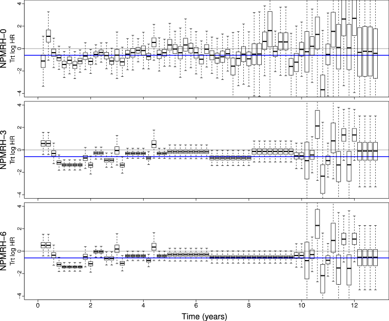
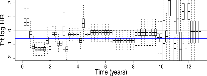
One of the most notable features of our results are in the estimated log-ratio of the treatment effect, particularly in the pruned models. In examining Figure 1, we note the interval-specific differences displayed in the caterpillar plots (top 3 plots in Figure 1). These plots reveal several important pieces of information about the treatment effects, including time periods where the treatment effects were: 1) proportional (constant) or non-proportional (changing), 2) statistically significantly different from previous periods, and 3) statistically significantly different from zero or from the proportional hazards model estimate of the treatment effect. For example, in the NPMRH-3 model, the treatment effects remained steady between (approximately): 6 ms-2 years, 3.5-4 years, 5-6.5 years, 6.5-8 years, and 8-10 years. However, these periods of constant estimated treatment effects were different from one another, suggesting that while the benefits of treatment lasted for a certain number of years, the degree of improvement changed (and generally declined) over the course of the study. Between 6 months and 2 years, long-term AD therapy had an estimated 75% improvement over short term AD therapy. In examining the 95% bounds of the boxplots, this estimated log-hazard ratio is statistically different than the log-ratio estimate from the proportional hazards model of (which translates to 45% improvement for the +24m group). Additionally, the estimated log-ratio in this time period is statistically significantly different than the estimated treatment effects between 5-6.5 and 8-10 years, which only showed an estimated 26% improvement for subjects on long-term therapy (see Figure 2, bottom). In both pruned models, the treatment effect held steady for a certain number of years, then diminished slightly, and held steady for another number of years, before diminishing in effectiveness again. Overall, long-term AD therapy did better in prolonging time to biochemical failure throughout most of the first 10 years of the study, despite the fact that in certain periods the log-ratio is not statistically significantly different from zero.
The results of all the MRH models provide two important insights: 1) The proportional hazards assumption indeed did not hold for treatment effects (agreeing with the Cox model test), and there were in fact periods of time where the estimated effects are statistically significantly different from each other, and 2) On average, the subjects on +24m of AD therapy experienced benefits for at least 10 years post treatment.
In Figure 1 (bottom right), we present the smoothed version of the caterpillar plots above, illustrating the overlap of the credible regions around the estimated log-hazard ratio for the four different models. The smoothing was done using a cubic smoothing spline (with 5 degrees of freedom, 53 knots, and a smoothing parameter equal to 0.82), which was implemented via the smooth.spline() function in R. While the caterpillar plots are useful for identifying specific interval differences in the treatment effect, these smoothed plots emphasize the difference in the uncertainty among the models and the different shapes of both the estimated effects and their credible intervals. For example, we see that among the NPMRH models, the unpruned model (NPMRH-0) has the widest credible interval bands, while the fully pruned model (NPMRH-6) has the narrowest credible interval bands, which is due to the smaller number of estimated parameters and larger failure counts per bin in the pruned model. While the PHMRH model clearly has the narrowest credible region, the constant parameter estimate cannot identify periods of increased or decreased long-term treatment benefit. This discrepancy is particularly visible in the last third of the study, where the benefits of long-term treatment seem to be decreasing.
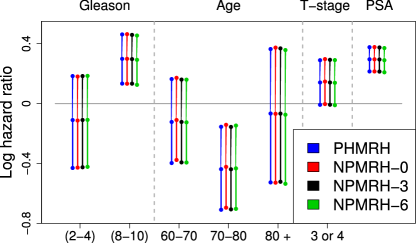
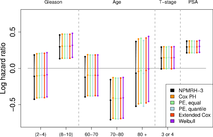
The estimates and their 95% credible intervals for the time-invariant effects (effects of age, Gleason scores, PSA measures, and T-stage) are almost identical among all the MRH models, and are shown in the “cat-scratch” plot in Figure 1, bottom left.
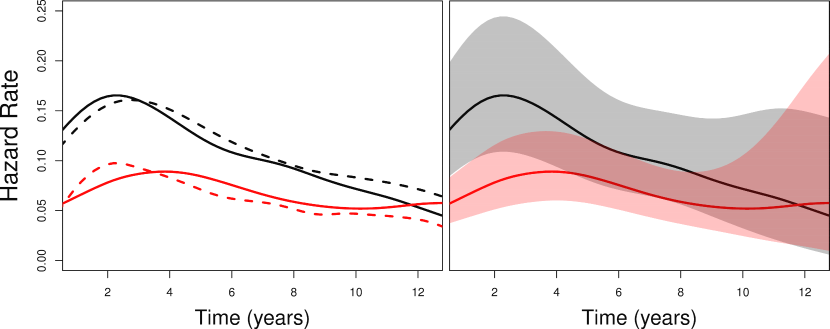
In all models, estimates of the biochemical failure hazard rate for each treatment group showed an increase in the first two to four years, with a steady decline afterwards (see Figure 2, upper left). However, subjects who received 24 months of additional AD therapy had a lower hazard rate than those who did not, with a flatter peak between 2 and 4 years. The non-proportionality between the hazards is particularly visible when compared to the results from the proportional hazards model. While both the NPMRH-3 and PHMRH models show similar estimated hazard rates for the +0m AD therapy group, the estimated hazard rates for the +24m group had significant departures in the first four to five years of the study, as well as in the last two years of the study. It does appear that, while long-term treatment effects diminished over time, biochemical failure was not simply postponed for the +24m group, but the risk was in fact reduced even over a longer period of time.
Time-invariant effect estimates show that an increase in Gleason scores was associated with an increased hazard rate, with a statistically significant difference between baseline subjects and subjects with scores greater than 8 (HR = 1.35, 95% CI: 1.14, 1.59). The hazard of biochemical failure decreased with age, although significant differences were only observed for subjects between 70 and 80 years old and baseline subjects (HR = 0.64, 95% CI: 0.49, 0.86). As expected, subjects with a T-stage of 3 or 4 had a higher hazard of biochemical failure compared to subjects with a T-stage equal to 2 (HR = 1.15 , 95% CI: 0.99, 1.34). Similarly, for every point increase in PSA scores on the log scale (a 2.7 factor increase in PSA measures on the standard PSA scale), there was a statistically significant 34% increase in the hazard rate. (See Table 2, Figure 1 bottom left.)
| Coefficient | 95% CI for | |||
|---|---|---|---|---|
| Gleason score | 2-4 | -0.11 | 0.90 | (-0.43, 0.18) |
| 8-10 | 0.30 | 1.35 | (0.13, 0.46) | |
| Age | -0.12 | 0.88 | (-0.39, 0.16) | |
| -0.44 | 0.64 | (-0.71, -0.16) | ||
| 80 or older | -0.07 | 0.94 | (-0.52, 0.37) | |
| T-stage 3 or 4 | 0.14 | 1.15 | (-0.01, 0.29) | |
| log(PSA), centered | 0.29 | 1.34 | (0.21, 0.37) | |
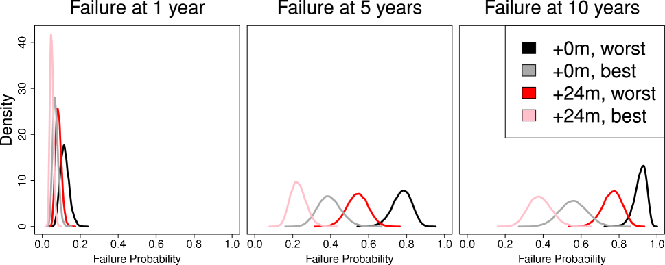
The probability of biochemical failure at 1, 5, and 10 years can be observed in Figure 3, which shows the smooth posterior predictive probability densities of biochemical failure, stratified by treatment type for hypothetical subjects with a“worst” or “best” covariate profile. A subject with a “worst” profile had a Gleason score , a T-stage 3 or 4 tumor, and a PSA score equal to 1 standard deviation greater than the mean (PSA ). A subject with a “best” profile had a Gleason score , a T-stage equal to 2, and a PSA score equal to 1 standard deviation below the mean (PSA ). At one year post diagnosis, we see that the posterior predictive densities were very similar among the four groups, all concentrated between 0 and 20%. However, by the 5-year post-diagnosis mark, the failure densities were very different. A worst profile subject on +0m AD therapy had failure probability centering around 80%, while a best profile subject on +24m of AD therapy had failure probability centering around 20%. It can also be observed that a worst profile subject had higher failure probability than a best profile subject, regardless of treatment type. The failure probability at 10 years post-diagnosis is perhaps the most telling, with a worst profile subject on +0m AD therapy having a failure probability ranging from 80-100%, which is a narrower range when compared to the other groups. Meanwhile, a best profile subject on +24m therapy had failure rates centering around 40%, over a wider interval from approximately 20% to 60%. While all posterior predictive densities overlapped at one year, at 5 and 10 years there was only a small amount of overlap between the best and worst profile subjects within the same treatment regimen.
4.2 Model Checking and Comparison
To assess the impact of different modeling and smoothness assumptions on the hazard of time to biochemical failure, we compared the four MRH models to each other as well as to other models, including the Cox proportional hazards model, a parametric non-proportional hazards Weibull model, two piece-wise exponential (PE) models, a dependent Dirichlet Process (DDP) survival model, and a semi-parametric Bayesian accelerated failure time (AFT) model, allowing for time-varying treatment effects in all models. In addition, we performed a sensitivity analysis to the parameter which controls the smoothness in the MRH tree prior (Bouman et al. (2005), see Appendix A for details). When applicable, models were compared through a goodness-of-fit measure (defined in Section 4.2.3), as well as via information criteria including BIC (Schwarz, 1978), AIC (Akaike, 1974), and DIC (Spiegelhalter et al., 2002; Celeux et al., 2006).
Cox Proportional Hazards Model
Because the Cox proportional hazards model is widely used in the analysis of survival data, we included this model as a comparison to other non-proportional hazards model for contrast (Cox, 1972). While we modeled the treatment effect under the proportional hazards assumption, it is important to note that the Schoenfeld residuals and methods presented by Grambsch and Therneau (1994) showed evidence that the treatment effect (long-term versus short-term therapy) was not proportional over the entire study period (see Figure 4). No other covariate effects showed evidence of non-proportionality over time.

Cox Model Extension
In addition to the traditional Cox proportional hazards model, we included an extended proportional hazards model with a time-varying treatment effect (Martinussen and Scheike, 2006). This extended Cox model has a hazard rate with the form
| (1) |
where is a -dimensional covariate, is a dimensional time-varying (i.e. NPH) regression coefficient that is estimated non-parametrically, and is the q-dimensional regression parameter for the PH covariate effects. An implementation of this model was performed using the timecox() function in the “timereg” package (Scheike, 2014), where parameters are estimated using score equations, and the optimal smoothing parameter was chosen based on the lowest -2*log-likelihood value and the lowest GOF scores.
Accelerated Failure Time Model
Accelerated failure time models are an alternative way to investigate the effects of non-proportional hazards. In our analysis, we used a Bayesian AFT model (Komárek and Lesaffre, 2007). This model can accommodate more complex clustered, interval-censored survival data, with the log of the survival times is modeled as:
where is the event time of the observation of the cluster. The model estimates the effects, , of the fixed effects and the i.i.d random effects . The fixed and random covariate effects are modeled using the classical Bayesian linear mixed model approach (such as Gelman et al. (2004)), and the hazard rate is approximated by normal mixtures. For the purposes of the prostate data, we omit any clustering effects.
Dependent Dirichlet Process Survival Model
As the most flexible alternative, we also consider a non-parametric Bayesian model that can accommodate non-proportional hazards. This model is based on the ANOVA Dependent Dirichlet Process (DDP) model presented in De Iorio et al. (2004), that has been extended to the survival analysis setting (De Iorio et al., 2009). The DDP survival model performs survival regression based on a Dirichlet Process prior.
The set of the random probability distributions or functions are dependent in an ANOVA-type fashion: If is the set of random distributions indexed by the categorical covariates , and the collection of random distributions is defined as
with and representing a point mass at then dependence is introduced by modeling the locations through the covariates (as explained in De Iorio et al. (2004) and De Iorio et al. (2009)). This model allows all group-specific hazards to be modeled non-proportionally, and covariate effects are interpreted in the standard ANOVA manner. The model is also capable of accommodating continuous covariates.
Because of the greater flexibility with the DDP survival model, this model is often unable to estimate all desired covariate effects. As a result, we present this model on a reduced set of variables that were found to be significant in other models: treatment, a high Gleason score, age between 70 and 80 years, and log(PSA).
Non-Proportional Hazards Weibull Model
The non-proportional effects Weibull model was designed with separate Weibull hazard rates for each treatment group and proportional hazard covariate effects shared among both treatment groups. Parameter estimates for this model were obtained using numerical optimization of the likelihood function:
where are the covariate effects modeled under the proportional hazards assumption. The estimate of the log-hazard ratio of the non-proportional effect of treatment at time in the Weibull model was then obtained as
where group 0 is the short-term treatment group, and group 1 is the long-term treatment group. The non-proportional hazards Weibull model parameter estimation was not performed using any available software packages, but is available on request from the authors.
Piece-wise Exponential Models
The piece-wise exponential (PE) model is a commonly used frequentist semi-parametric model for joint estimation of the hazard rate and covariate effects (for example, see Friedman (1982)). It is similar to the MRH model in that both assume constant hazard rates within a time bin (), but it does not have the multi-resolution aspects of MRH.
As with the non-proportional hazards Weibull model, we fit a PE model with separate hazard rates for each treatment group, and shared proportional hazards effects among all subjects. If we let represent the constant hazard rate in the bin for the treatment group ( and ), then the piece-wise exponential likelihood can be written as:
where
To make the PE model comparable with the pruned MRH models, we use a data-driven method to select the optimal number of bins as well as the optimal bin width(s). In addition, we modify the standard PE approach slightly in order to overcome a common obstacle in the estimation of the variance. Namely, given that the Fisher Information for the hazard rate in bin for group can be derived as:
bins with no observed failures will yield of zero, making the Fisher Information matrix singular. In such instances, we have remedied this issue by (repeated) merging of the bins with no observed failures into the adjacent bins to the left. With that modification, for each of the hazard rates, we find the PE model with the optimal number of bins and bin widths based on an information criterion such as AIC (Akaike, 1974), in two ways:
-
1.
Equal-bin model: The “equal-bin” PE model partitions the time axis evenly into bins (where ). Among the equal-bin PE models, we retain the model that has the lowest AIC value.
-
2.
Quantile-bin model: The “quantile-bin” PE model partitions the time axis into quantiles (). Among the quantile-bin PE models, we retain the model that has the lowest AIC value.
In the RTOG 92-02 data set, the final equal-bin PE model had 17 bins for the +0m treatment group hazard rate and 18 bins for the +24m treatment group hazard rate. The last three bins were combined for the +0m treatment group, and the last two bins had to be combined for the +24m treatment group hazard rate. (Note that as the result, not all bins were of equal length due to the combined bins at the end of the study). The final quantile-bin model had 24 bins for the +0m treatment group hazard rate and 25 bins for the +24m treatment group hazard rate. The last three bins were combined for the +0m treatment group, and the last two bins were combined for the +24m treatment group.
4.2.1 Comparison of Estimated Hazard Ratio and Predictor Effects
The estimates from all models are compared visually in Figures 6 and 5. All models were remarkably similar in terms of the proportional hazard covariate effects, both in point estimates and their 95% bounds (credible intervals for the MRH model, and confidence intervals for the remaining models), as can be seen in Figure 5. Given this similarity, we refer the readers to Table 2 and Section 4.1 for interpretation and discussion of these effects in the NPMRH-3 model. (Note that the estimated covariate effects for the AFT and DDP survival models are not shown as their number and interpretation are different than the other models.)
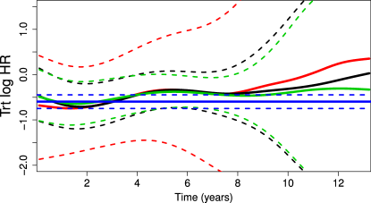
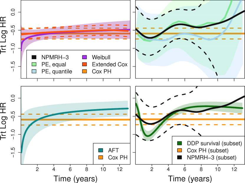
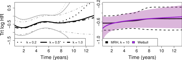
In contrast, the estimates of the time-varying treatment effect show notable differences (Figure 6). The PE and MRH models provide similar estimates, although the PE model log-HR estimates exhibit a rapid increase towards the end of the study when the number of observed failures becomes sparse (top right graph). Due to its parametric form, the NPH Weibull model has an initial dip in the estimated treatment effect, and then slowly but steadily increases over the course of the study, although the estimated effects remain negative throughout the study period. The extended Cox model shows a similar pattern and estimate, without the initial dip (top left graph). The AFT estimated log-HR follows a trajectory similar to that of the NPH Weibull model, including the wider 95% confidence interval bounds in the initial study period (bottom left graph). The DDP survival model (calculated on the subset of significant predictors only) shows an initial pattern similar to that of the NPMRH-3 model (also calculated on the subset of significant predictors only), with a dip at the two year mark, followed by an upward trend. The DDP survival model is the only model that shows a possible decreasing trend towards the end of the study. For comparison, the Cox PH model treatment estimate (included under the proportional hazards assumption), has been included in all graphs as a constant value over time (, 95% CI: -0.74, -0.44). It can be observed that throughout various periods of the study, all models have estimated treatment effects that extend outside the 95% confidence interval for the Cox PH model treatment effect. In addition, all models show that long-term treatment is beneficial over longer periods of time, even if the effects may be diminishing.
4.2.2 Sensitivity Analysis to Parameter in the MRH Models
In all the MRH models, the parameter controls the correlation among the hazard increments within each bin (Bouman et al. (2005), see Appendix A for details). The default value for in the above analyses was 0.5, which implies zero a priori correlation among the hazard increments. However, when , the increments are positively correlated a priori, and, similarly, when the hazard increments are negatively correlated a priori. Another way to understand the impact of is that higher values lead to smoother hazard functions.
In practice, different approaches to choosing a hyperprior for , including empirical Bayes methods, are possible. However, will in general tend to depend on the resolution level (Bouman et al., 2005), as well as with the significance level used in the pruning algorithm (Chen et al., 2014). Both the resolution and the pruning can be also used to imply the desired a priori level of smoothness of the hazard function. For this reason, we fix in the above analyses, and perform a sensitivity analysis to examine the effect the choice of k might have on the posterior hazard rate estimates. We only examine the effects of different values of in the 3-level pruned MRH model (NPMRH-3) (see Subsection 4.2.3 for motivation.)
The sensitivity analysis results are displayed in Figure 7. On the left plot in Figure 7, the original NPMRH-3 model (with ) is contrasted against the models with negatively correlated hazard increments (), and positively correlated hazard increments (). As anticipated, in the negatively correlated model the log-HR is less smooth, and has wider 95% credible intervals, resembling the PE model results. However, the NPMRH-3 model with is smoother, with narrower 95% credible intervals. The positive correlation between hazard increments results in smoother posterior estimates, as more information is shared across bins. The right graph of Figure 7 highlights the adaptability of the MRH model in controlling the smoothness of the log-hazard ratio through the parameter . In this instance, with fixed at a very high value of 10 (highly positively correlated increments), the NPMRH-3 model closely mimics the results of the parametric NPH Weibull model.
4.2.3 Model Performance Comparison
In addition to model parameter comparisons in Subsection 4.2.1, the set of models were also compared based on their goodness of fit (GOF), as well as several information criteria. The GOF was evaluated using the following simple measure over time:
where denotes absolute value, is an indicator variable which equals if the subject fails after time and equals 0 otherwise, and is the model-based probability of the subject experiencing biochemical failure. This probability is found based on the estimated model parameters (posterior medians, or maximum likelihood estimates) and covariates for subject . Patients who were censored before time were not included in the GOF calculation at time . Therefore, represents the total number of patients in the cohort minus the number of patients censored before time , so that the maximum value the GOF statistic can take is 1. In other words, the GOF measure calculates the average difference between the observed failure time and the probability of failure at that time point. Lower GOF values indicate more accurate failure approximations and a better fitting model.
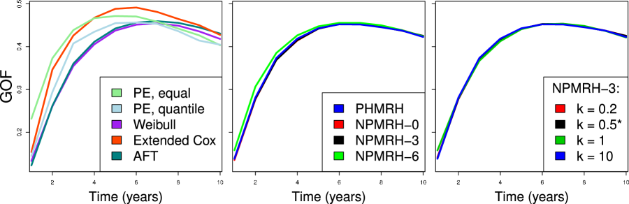
Results from the GOF statistic calculations are shown in Figure 8. Most models show very similar results and trajectories, with exception for both of the adjusted PE models and the extended Cox model. The adjusted PE model with equal bins has the worst survival prediction initially, followed by the extended Cox model and the adjusted PE model with bins determined through quantiles. After four years, the extended Cox model has the highest GOF of all models. Differences between the MRH models (including those with different values of the prior parameter ) are negligible, and also very similar to the results for the NPH Weibull and AFT models. Note that the GOF statistic was not calculated for the Cox proportional hazards model, as no estimate of the hazard rate is typically produced by Cox models. That statistic was also not calculated for the DDP survival model, as subject-specific survival curves are not provided in that package.
Table 3 shows several information criteria (AIC, BIC, and DIC where appropriate) for all the models considered (with the exception of the DDP survival model, as subject-specific hazard rates and survival curves are not provided in that package). Among the MRH models, the PHMRH model has the highest DIC value, which is about 5000 points greater than any of the NPMRH models. It also has the highest negative log-likelihood, BIC and AIC values, despite the smaller number of parameters when compared to the NPMRH models. This is consistent with our earlier observation that the PH model does not seem to provide a good description of the data.
When comparing the NPMRH models with different levels of pruning (NPMRH-0, NPMRH-3, NPMRH-6), the NPMRH-3 model has the lowest negative log-likelihood value, followed closely by the NPMRH-6 model. The NPMRH-6 model has the lowest DIC, BIC, and AIC values as it has the smallest number of estimated parameters of all MRH models considered. However, all three NPMRH models have very similar information criteria values, with the exception of BIC for NPMRH-0 whose penalty for its large number of parameters sets it apart from the rest of the models. It is also notable that among the NPMRH-3 models, the lowest negative log-likelihood, DIC, BIC, and AIC values are for the model with , which may be a good choice for examining the hazard rate of biochemical failure for this particular data set, as it captures the most details in the failure pattern. The negative log-likelihood values (and hence BIC and AIC calculations) of the adjusted PE models are slightly smaller than those of the NPMRH models, although the values are comparable. When compared to the NPH Weibull models, the NPMRH models all have lower negative log-likelihood values. However, BIC and AIC values are higher in the NPMRH models due to the higher number of estimated parameters. The AFT model has a higher negative log-likelihood value when compared to the other models (with the exception of the PHMRH model), and the extended Cox model has a slightly higher negative log-likelihood value when compared to the MRH models, but the values are similar. Regardless of model choice however, all evidence points to the treatment effects not being proportional: the effects of an additional 24 months of AD therapy change over the entire length of the study.
| Model | -2*log(L) | Effective Number | DIC | BIC | AIC | |
| of Parameters | ||||||
| MRH | PHMRH | 12628.0 | 32 | 9651.1 | 12860.3 | 10555.8 |
| NPMRH-0 | 4703.1 | 139 | 4751.5 | 5712.1 | 4981.1 | |
| NPMRH-3 | 4669.8 | 43 | 4665.0 | 4981.9 | 4755.8 | |
| NPMRH-6 | 4679.0 | 38 | 4602.1 | 4954.8 | 4755.0 | |
| NPMRH-3 () | 4667.9 | 43 | 3582.9 | 4980.1 | 4753.9 | |
| NPMRH-3 () | 4669.8 | 43 | 4665.0 | 4981.9 | 4755.8 | |
| NPMRH-3 () | 4700.7 | 43 | 4298.7 | 5012.9 | 4786.7 | |
| NPMRH-3 () | 4792.8 | 43 | 4578.2 | 5105.0 | 4878.8 | |
| PE | Equal bins | 4611.1 | 42 | - | 4916.0 | 4695.1 |
| Quantile bins | 4596.7 | 56 | - | 5003.2 | 4708.7 | |
| NPH Weibull | 4759.9 | 11 | - | 4839.7 | 4781.9 | |
| AFT | 5277.9 | - | - | - | - | |
| Extended Cox | 4747.0 | - | - | - | - | |
5 Discussion
This paper illustrates how different modeling and smoothing assumptions effect the estimate of the time-varying treatment effect. We present results from a suite of models ranging from parametric to non-parametric, and demonstrate that different assumptions can lead to very smooth, flat log-hazard ratio estimates (such as those in the NPH Weibull model) to estimates which vary more over time (such as those in the MRH, PE, and the DDP survival model). Additionally, the different models exhibited a high degree of variability in the goodness-of-fit measure and the penalized goodness of fit criteria. We have also shown how choosing different values of gives the MRH model the flexibility to perform similarly to other models, ranging from the piece-wise exponential to the parametric Weibull model. The NPMRH model allows for multiple changes in the treatment effects over time, with multiple increases and decreases over the length of a study period.
Other patient and disease characteristic covariate effects were similar to those previously seen in this trial (Horwitz et al., 2008) and expected based on the effects of these factors in other studies. Men with higher Gleason scores had greater hazard of biochemical failure, although this difference was statistically significant only for those with Gleason scores of 8 or more. In addition, those with more advanced tumor stage (T-stage 3 or 4) or with higher PSA level at diagnosis also had a higher hazard rate of biochemical failure. Men who were older at diagnosis were found to have a lower hazard rate of biochemical failure, although this may be still partly confounded with the censoring patterns in older patients and warrants further exploration.
Additionally, the presented analysis has allowed insight into the effects of the duration of AD therapy on biochemical failure, and in particular into how the effects of AD therapy changed throughout the course of the study. While it was already apparent that 24 months of additional AD therapy is beneficial (relative to the 0 additional months of AD therapy) in that it prolongs the time until biochemical failure and other failure endpoints (Horwitz et al., 2008), our investigation has revealed additional insights. During and immediately after active therapy, the peak in the hazard rate around two years is much flatter for the +24m treatment group. In addition, the +24 month group continued to have a lower hazard rate throughout most of the observation period (over 10 years), although smaller due to the non-proportionality of the treatment effect. Thus, it does appear that the benefits of the additional months of AD therapy, while diminishing over time, are persistent, which suggests that failure in the longer AD duration group are not simply deferred but possibly avoided. On the other hand, for those patients who received short AD therapy and did not fail early or during the peak period of failures, their late term prognosis is nearly as favorable as those who underwent long duration AD. Thus, until such patients can be prospectively identified, the long AD approach would seem to be preferred for all patients. To this end, we also illustrate how the Bayesian approach can allow the use of posterior predictive failure probabilities, such as in Figure 3, as aids in clinical contexts.
Appendix A: Details on the MRH prior and Pruning Method
MRH prior
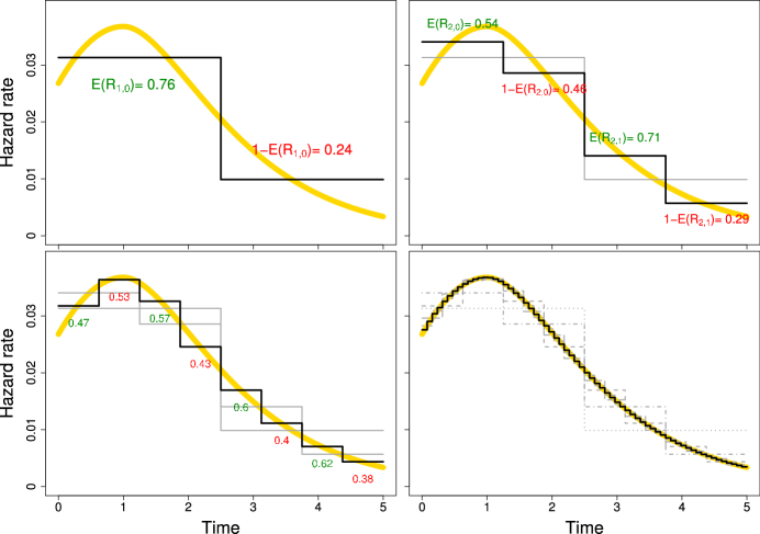
The foundation of the MRH method is a tree-like wavelet-based multi-resolution prior on the hazard function, chosen conveniently to allow scalability and consistency across different time scales (i.e minutes, weeks, years, etc). It uses a piece-wise constant approximation of the hazard function over time intervals, parametrized by a set of hazard increments . Here, each represents the aggregated hazard rate over the time interval, ranging from . In the standard survival analysis notation, , where is the hazard rate at time .
To facilitate the recursive diadic partition of the multiresolution tree, we assume that . Here, is an integer, set large enough to achieve the desired time resolution for the hazard rate. can also be chosen using model selection criteria or clinical input, as in Bouman et al. (2005), and Dignam et al. (2009). Note that the cumulative hazard, , is equal to the sum of all hazard increments . The model then recursively splits at different branches via the “split parameters” . Here, is recursively defined as (with , and ). The split parameters, each between 0 and 1, guide the shape of the a priori hazard rate over time (Figure 9).
The complete hazard rate prior specification is obtained via priors placed on all tree parameters: a Gamma() prior is placed on the cumulative hazard , and Beta prior on each split parameter , . For example, the priors for and in 3-level MRH model () would be:
| (2) |
Under this parametrization, the prior distribution of each hazard increment is governed by these Beta and Gamma distributions. In particular, their prior expectations depend on the hyperparameters of the Beta and Gamma priors – for example, in the above 3-level model . Similarly, these MRH hyperparameters control the correlation between the hazard increments , and thus directly relate to the smoothness of the multiresolution prior, as shown in Bouman et al. (2005) and Chen et al. (2014). This parametrization also insures the self-consistency of the MRH prior at multiple resolutions (Bouman et al., 2005; Chen et al., 2014).
Pruning the MRH tree
The MRH prior resolution is chosen as a compromise between the desire for detail in the hazard rate, and the amount of data. As the resolution increases (and the number of time intervals increases), observed failure counts within each bin will decrease. While useful for revealing detailed patterns, a large number of intervals (and consequently, a large number of model parameters) will generally require longer computing times and result in estimators with lower statistical efficiency (Chen et al., 2014). “Pruning”, as used in Chen et al. (2014), is a data-driven pre-processing technique, which combines consecutive s that are statistically similar (and happens frequently with periods of low failure counts). The technique increases the computational efficiency by decreasing the parameter dimension a priori, which can greatly speed up analyses of non-proportional hazards. The pruning method thus changes the overall time resolution of the MRH prior, keeping the higher resolution during the periods of high event counts, and lower resolution during periods of low event counts.
The MRH pruning technique has been extensively studied in Chen et al. (2014). Briefly, pruning starts with the full MRH tree prior, and merges adjacent bins that are constructed via the same split parameter, , when the hazard increments in these two bins ( and ) are statistically similar. This is inferred by testing the hypothesis against the alternative , with a pre-set type I error , for each split parameter (). If the null hypothesis is not rejected, that split is set to and the adjacent hazard increments are considered equal and the time bins declared “fused”. The hypothesis testing can be applied to all levels of the tree or just a higher resolution subset of the tree. While the pruning is expected to reduce the amount hazard rate detail discovered by the MRH method, the posterior hazard rate estimator is shown to have lower risk compared to its equivalent from the non-pruned model (Chen et al., 2014).
Appendix B: Estimation and Pruning Steps
The estimation algorithm is performed two steps: the pruning step and the Gibbs sampler routine. The details are listed below.
Pruning step
The pruning step is run only once for each of the hazard rates at the beginning of the algorithm as a pre-processing step in order to finalize the MRH tree priors. The parameters for which the null hypothesis is not rejected are set to with probability 1, while the rest are estimated in the Markov chain Monte Carlo (MCMC) routine.
Gibbs sampler steps
After the pruning step, the Gibbs sampler algorithm is performed to obtain the approximate posterior distribution of , and the that have not been set to 0.5 for each stratum () as well as .
The algorithm is as follows, with steps repeated until convergence:
-
1.
For each of the treatment hazard rates ():
-
(a)
Sample from the posterior for , which is a gamma density with the shape parameter , and rate parameter , where = .
-
(b)
Sample from their respective posterior distributions (see below).
-
(c)
Sample each for which the null hypothesis was rejected from the full conditional:
-
(d)
Sample from their respective posterior distributions (see below).
-
(a)
-
2.
With a prior (with a known variance) on each covariate effect modeled under the proportional hazards assumption, ), each has the following full conditional distribution:
Note that this posterior distribution includes the full set of observations and covariates, from all strata jointly.
Full conditionals for the hyperparameters , and
The parameters in the prior distributions of and all s for each covariate stratum (), , and , can either be fixed at desired values, or treated as random variables with their own set of hyperpriors. In the case of the latter, they would be sampled within the Gibbs sampler separately for each stratum, according to their own full conditional distributions. Below are the forms of these full conditional distributions for a specific set of hyperpriors we chose.
For notational simplicity, the stratum-specific index is suppressed below. The notation will be used to denote the set of all data and all parameters except for the parameter itself. The full conditionals are as follows:
-
•
If is given a zero-truncated Poisson prior, (chosen for computational convenience), the full conditional distribution for is:
-
•
If the scale parameter in the gamma prior for the cumulative hazard function is given an exponential prior with mean , the resulting full conditional is:
-
•
If is given an exponential prior distribution with mean , the full conditional distribution for is as follows:
-
•
If a Beta(, ) prior is placed on each , the full conditional distribution for each is proportional to:
References
- Akaike (1974) Akaike, H. “A new look at the statistical model identification.” IEEE Transactions on Pattern Analysis and Machine Intelligence, 19:716–723 (1974).
- Albertsen et al. (2005) Albertsen, P., Hanley, J., and Fine, J. “20-year outcomes following conservative management of clinically localized prostate cancer.” The Journal of the American Medical Association, 293:2095–2101 (2005).
- American Joint Committee on Cancer (2014) American Joint Committee on Cancer. “What is cancer staging?” http://cancerstaging.org/references-tools/Pages/What-is-Cancer-Staging.%aspx (2014). Date accessed: October 1, 2014.
- Amling et al. (2000) Amling, C., Blute, M., Bergstralh, E., Seay, T., Slezak, J., and Zincke, H. “Long-term hazard of progression after radical prostatectomy for clinically localized prostate cancer: Continued risk of biochemical failure after 5 years.” The Journal of Urology, 164:101–105 (2000).
- Andersen et al. (1993) Andersen, P., Borgan, O., Gill, R., and Keiding, N. Statistical Methods Based on Counting Processes. Berlin: Springer-Verlag (1993).
- Arjas and Gasbarra (1994) Arjas, E. and Gasbarra, D. “Nonparametric Bayesian inference from right censored survival data, using the Gibbs sampler.” Statistica Sinica, 4:505–524 (1994).
- Barry (2001) Barry, M. “Prostate-Specific-Antigen testing for early diagnosis of prostate cancer.” The New England Journal of Medicine, 344:1373–1377 (2001).
- Berry et al. (2004) Berry, S., Berry, D., Natarajan, K., Lin, C., Hennekens, C., and Belder, R. “Bayesian survival analysis with nonproportional hazards.” Journal of the American Statistical Association, 99:515–526 (2004).
- Bouman et al. (2007) Bouman, P., Dignam, J., Dukic, V., and Meng, X. “A multiresolution hazard model for multi-center survival studies: Application to Tamoxifen treatment in early stage breast cancer.” Journal of the American Statistical Association, 102:1145–1157 (2007).
- Bouman et al. (2005) Bouman, P., Dukic, V., and Meng, X. “Bayesian multiresolution hazard model with application to an AIDS reporting delay study.” Statistica Sinica, 15:325–357 (2005).
- Brawer et al. (1992) Brawer, M., Chetner, M., Beatie, J., Buchner, D., Vessella, R., and Lange, P. “Screening for prostatic carcinoma with prostate specific antigen.” Journal of Urology, 147:841–845 (1992).
- Brooks and Gelman (1998) Brooks, S. and Gelman, A. “General methods for monitoring convergence of iterative simulations.” Journal of Computational and Graphical Statistics, 7:434–455 (1998).
- Buckley and James (1979) Buckley, J. and James, I. “Linear regression with censored data.” Biometrika, 66:429–436 (1979).
- Burridge (1981) Burridge, J. “Empirical Bayes Analysis of Survival Time Data.” Journal of the Royal Statistical Society - Series B, 43:65–75 (1981).
- Buyyounouski et al. (2008) Buyyounouski, M., Hanlon, A., Horwitz, E., and Pollack, A. “Interval to biochemical failure highly prognostic for distant metastasis and prostate cancer-specific mortality after radiotherapy.” International Journal of Radiational Oncology*Biology*Physics, 70:59–66 (2008).
- Cai and Meyer (2011) Cai, B. and Meyer, R. “Bayesian semi parametric modeling of survival data based on mixtures of B-spline distributions.” Computational Statistics and Data Analysis, 55:1260–1272 (2011).
- Catalona et al. (1991) Catalona, W., Smith, D., Ratliff, T., Dodds, K., Coplan, D., Yuan, J., Petros, J., and Andriole, G. “Measurement of Prostate-Specific Antigen in serum as a screening test for prostate cancer.” The New England Journal of Medicine, 324:1156–1161 (1991).
- Celeux et al. (2006) Celeux, G., Forbes, F., Robert, C., and Titterington, D. “Deviance information criteria for missing data models.” Bayesian Analysis, 1:651–673 (2006).
- Chakravarti et al. (2007) Chakravarti, A., DeSilvio, M., Zhang, M., Grignon, D., Rosenthal, S., Asbell, S., Hanks, G., Sandler, H., Khor, L., Pollack, A., and Shipley, W. “Prognostic value of p16 in locally advanced prostate cancer: A study based on Radiation Therapy Oncology Group protocol 9202.” Journal of Clinical Oncology, 25:3082–3089 (2007).
- Che et al. (2007) Che, M., DeSilvio, M., Pollack, A., Grignon, D., Venkatesan, V., Hanks, G., and Sandler, H. “Prognostic value of abnormal p53 expression in locally advanced prostate cancer: A study based on RTOG 9202.” International Journal of Radiational Oncology*Biology*Physics, 69:1117–1123 (2007).
- Chen et al. (2014) Chen, Y., Hagar, Y., Dignam, J., and Dukic, V. “Pruned Multiresolution Hazard (PMRH) Models for Time-to-Event Data.” Bayesian Analysis, In Review (2014).
- Cooner et al. (1990) Cooner, W., Mosley, B., Rutherford, C., Beard, J., Pond, H., Terry, W., Igel, T., and Kidd, D. “Prostate cancer detection in clinical urological practice by ultrasonography, digital rectal examination and Prostate Specific Antigen.” Journal of Urology, 143:1146–1152 (1990).
- Cox (1972) Cox, D. “Regression Models and Life-Tables.” Journal of the Royal Statistical Society - Series B, 34:187–220 (1972).
- Dabrowska et al. (1989) Dabrowska, D., Doksum, K., and Song, T. “Graphical comparison of cumulative hazards for two populations.” Biometrika, 76:763–773 (1989).
- D’Amico et al. (2003) D’Amico, A., Moul, J., Carroll, P., Sun, L., Lubeck, D., and Chen, M. “Surrogate end point for prostate cancer - specific mortality after radical prostatectomy or radiation therapy.” Journal of the National Cancer Institute, 95:1376–1383 (2003).
- De Iorio et al. (2009) De Iorio, M., Johnson, W., Müller, P., and Rosner, G. “Bayesian nonparametric nonproportional hazards survival modeling.” Biometrics, 65:762–771 (2009).
- De Iorio et al. (2004) De Iorio, M., Müller, P., Rosner, G., and MacEachern, S. “An ANOVA model for dependent random measures.” Journal of the American Statistical Association, 99:202–215 (2004).
- Dignam et al. (2009) Dignam, J., Dukic, V., Anderson, S., Mamounas, E., Wickerham, D., and Wolmark, N. “Hazard of recurrence and adjuvant treatment effects over time in lymph node-negative breast cancer.” Breast Cancer Research and Treatment, 116:595–602 (2009).
- Dillioglugil et al. (1997) Dillioglugil, O., Leibman, B., Kattan, M., Seal-Hawkins, C., Wheeler, T., and Scardino, P. “Hazard rates for progression after radical prostatectomy for clinically localized prostate cancer.” Adult Urology, 50:93–99 (1997).
- Dong and Matthews (2012) Dong, B. and Matthews, D. “Empirical likelihood for cumulative hazard ratio estimation with covariate adjustment.” Biometrics, 68:408–418 (2012).
- Dukic and Dignam (2007) Dukic, V. and Dignam, J. “Bayesian hierarchical multiresolution hazard model for the study of time-dependent failure patterns in early stage breast cancer.” Bayesian Analysis, 2:591–610 (2007).
- Epstein et al. (2005) Epstein, J., Jr., W. A., Amin, M., Egevad, L., and the ISUP Grading Committee. “The 2005 International Society of Urological Pathology (ISUP) Concensus Conference on Gleason grading of prostatic carcinoma.” American Journal of Surgical Pathology, 29:1228–1242 (2005).
- Ferguson (1974) Ferguson, T. “Prior distributions on spaces of probability measures.” The Annals of Statistics, 2:615–629 (1974).
- Friedman (1982) Friedman, M. “Piecewise exponential models for survival data with covariates.” Annals of Statistics, 10:101–113 (1982).
- Gelman et al. (2004) Gelman, A., Carlin, J., Stern, H., and Rubin, D. Bayesian Data Analysis, 2nd edition. Chapman and Hall/CRC, Boca Raton (2004).
- Gelman and Rubin (1992) Gelman, A. and Rubin, D. “Inference from iterative simulation using multiple sequences.” Statistical Science, 7:457–511 (1992).
- Geweke (1992) Geweke, J. Evaluating the accuracy of sampling-based approaches to calculating posterior moments in Bayesian Statistics 4. Clarendon Press, Oxford, UK (1992).
- Grambsch and Therneau (1994) Grambsch, P. and Therneau, T. “Proportional hazards tests and diagnostics based on weighted residuals.” Biometrika, 81:515–526 (1994).
- Gray (1990) Gray, R. “Some diagnostic methods for Cox regression models through hazard smoothing.” Biometrics, 46:93–102 (1990).
- Gray (1992) —. “Flexible methods for analyzing survival data using splines, with applications to breast cancer prognosis.” Journal of the American Statistical Association, 87:942–951 (1992).
- Gray (1996) —. “Hazard rate regression using ordinary nonparametric regression smoothers.” Journal of Computational and Graphical Statistics, 5:190–207 (1996).
- Hagar et al. (2014a) Hagar, Y., Albers, D., Pivavarov, R., Chase, H., Dukic, V., and Elhadad, N. “Survival analysis with Electronic Health Record data: Experiments with Chronic Kidney Disease.” Statistical Analysis and Data Mining, 7:385–403 (2014a).
- Hagar et al. (2014b) Hagar, Y., Chen, Y., and Dukic, V. “MRH package in R.” http://cran.r-project.org/web/packages/MRH/index.html (2014b).
- Hanlon and Hanks (2000) Hanlon, A. and Hanks, G. “Failure patterns and hazard rates for failure suggest the cure of prostate cancer by external beam radiation.” Adult Urology, 55:725–729 (2000).
- Hanson (2006) Hanson, T. “Inference for mixtures of finite Polya tree models.” Journal of the American Statistical Association, 101:1548–1565 (2006).
- Hanson and Johnson (2002) Hanson, T. and Johnson, W. “Modeling regression error with a mixture of Polya trees.” Journal of the American Statistical Association, 97:1020–1033 (2002).
- Held-Warmkessel (2006) Held-Warmkessel, J. Contemporary Issues in Prostate Cancer. Sudbury, Massachusettes: Jones and Bartlett Publishers (2006).
- Hennerfeind et al. (2006) Hennerfeind, A., Brezger, A., and Fahrmeir, L. “Geoadditive Survival Models.” Journal of the American Statistical Association, 101:1065–1075 (2006).
- Hess (1994) Hess, K. “Assessing time-by-covariate interactions in proportional hazards regression models using cubic spline functions.” Statistics in Medicine, 13:1045–1062 (1994).
- Hjort (1990) Hjort, N. “Nonparametric Bayes estimators based on beta processes in models for life history data.” Annals of Statistics, 18:1259–1294 (1990).
- Holford (1976) Holford, T. “Life tables with concomitant information.” Biometrics, 32:587–597 (1976).
- Holford (1980) —. “The analysis of rates and of survivorship using log-linear models.” Biometrics, 36:299–305 (1980).
- Horwitz et al. (2008) Horwitz, E., Bae, K., Hanks, G., Porter, A., Grignon, D., Brereton, H., Venkatesan, V., Lawton, C., Rosenthal, S., Sandler, H., and Shipley, W. “Ten-year follow-up of Radiation Therapy Oncology Group protocol 92-02: a phase III trial of the duration of elective androgen deprivation in locally advanced prostate cancer.” (2008).
- Ibrahim et al. (2001) Ibrahim, J., Chen, M., and Sinha, D. Bayesian Survival Analysis. New York: Springer (2001).
- Jara et al. (2012) Jara, A., Hanson, T., Quintana, F., Mueller, P., and Rosner, G. “DPpackage package in R.” cran.r-project.org/web/packages/DPpackage/DPpackage.pdf (2012).
- Kalbfleisch (1978) Kalbfleisch, J. “Non-parametric Bayesian Analysis of survival time data.” Journal of the Royal Statistical Society - Series B, 40:214–221 (1978).
- Kalbfleisch and Prentice (2002) Kalbfleisch, J. and Prentice, R. The Statistical Analysis of Failure Time Data. Chichester: SWiley (2002).
- Komárek (2015) Komárek, A. “bayesSurv package in R.” http://cran.r-project.org/web/packages/bayesSurv/bayesSurv.pdf (2015).
- Komárek and Lesaffre (2007) Komárek, A. and Lesaffre, E. “Bayesian Accelerated failure time model for correlated interval-censored data with a normal mixture as error distribution.” Statistica Sinica, 17:549–569 (2007).
- Laird and Olivier (1981) Laird, N. and Olivier, D. “Covariance analysis of censored survival data using log-linear analysis techniques.” Journal of the American Statistical Association, 76:231–240 (1981).
- Lavine (1992) Lavine, M. “Some aspects of Polya tree distributions for statistical modelling.” The Annals of Statistics, 20:1222–1235 (1992).
- Lee and Kim (2004) Lee, J. and Kim, Y. “A new algorithm to generate beta processes.” Computational Statistics and Data Analysis, 47:441–453 (2004).
- Martinussen and Scheike (2006) Martinussen, T. and Scheike, T. Dynamic Regression Models for Survival Data. New York, NY: Springer (2006).
- McKeague and Zhao (2002) McKeague, I. and Zhao, Y. “Simultaneous confidence bands for ratios of survival functions via empirical likelihood.” Statistics and Probability Letters, 60:405–415 (2002).
- Moyer (2012) Moyer, V. “Screening for prostate cancer: U.S. Preventive Services Task Force recommendation statement.” Annals of Internal Medicine, 157:120–135 (2012).
- Muliere and Walker (1997) Muliere, P. and Walker, S. “A Bbayesian non-parametric approach to survival analysis using Polya trees.” Scandinavian Journal of Statistics, 24:331–340 (1997).
- Müller and Rodriguez (2013) Müller, P. and Rodriguez, A. Nonparametric Bayesian Inference. Beachwood, Ohio and Alexandria, Virginia, USA: Institute of Mathematical Statistics and American Statistical Association (2013).
- Nguyen et al. (2013) Nguyen, Q., Levy, L., Lee, A., Choi, S., Frank, S., Pugh, T., McGuire, S., Hoffman, K., and Kuban, D. “Long-term outcomes for men with high-risk prostate cancer treated definitively with external beam radiotherapy with or without androgen deprivation.” Cancer, 119:3265–71 (2013).
- Nieto-Barajas (2014) Nieto-Barajas, L. “Bayesian semiparametric analysis of short- and long-term hazard ratios with covariates.” Computational Statistics and Data Analysis, 71:477–490 (2014).
- Nieto-Barajas and Müller (2012) Nieto-Barajas, L. and Müller, P. “Rubbery Polya tree.” Scandinavian Journal of Statistics, 39:166–184 (2012).
- Nieto-Barajas and Walker (2002) Nieto-Barajas, L. and Walker, S. “Markov beta and gamma processes for modeling hazard rates.” Scandinavian Journal of Statistics, 29:413–424 (2002).
- Parzen et al. (1997) Parzen, M., Wei, L., and Ying, Z. “Simultaneous confidence intervals for the difference of two survival functions.” Scandinavian Journal of Statistics, 24:309–314 (1997).
- Pilepich et al. (2001) Pilepich, M., Winter, K., John, M., Mesic, J., Sause, W., Rubin, P., Lawton, C., Machtay, M., and Grignon, D. “Phase III Radiation Therapy Oncology Group (RTOG) trial 86-10 of androgen deprivation adjuvant to definitive radiotherapy in locally advanced carcinoma of the prostate.” International Journal of Radiational Oncology*Biology*Physics, 50:1243–1252 (2001).
- Pilepich et al. (2005) Pilepich, M., Winter, K., Lawton, C., Krisch, R., Wolkov, H., Movsas, B., Asbell, E. H. S., and Grignon, D. “Androgen suppression adjuvant to definitive radio- therapy in prostate carcinoma: Long-term results of phase III RTOG 85-31.” International Journal of Radiational Oncology*Biology*Physics, 61:1285–1290 (2005).
- Radiation Therapy Oncology Group (2014a) Radiation Therapy Oncology Group. “RTOG 9202 Protocol Information.” http://www.rtog.org/ClinicalTrials/ProtocolTable/StudyDetails.aspx?stud%y=9202 (2014a). Last Updated: March 11, 2014.
- Radiation Therapy Oncology Group (2014b) —. “RTOG History.” http://www.rtog.org/AboutUs/History.aspx (2014b). Last Accessed: October 10, 2014.
- Roach et al. (2007) Roach, M., III, De Silvio, M., Rebbick, T., Grignon, D., Rotman, M., Wolkov, H., Fisher, B., Hanks, G., Shipley, W., Pollack, A., Sandler, H., and Watkins-Bruner, D. “Racial differences in CYP3A4 Genotype and Survival among men treated on Radiation Therapy Oncology Group (RTOG) 9202: A Phase III randomized trial.” International Journal of Radiational Oncology*Biology*Physics, 69:79–87 (2007).
- Roach et al. (2006) Roach, M., III, Hanks, G., Thames, H., Jr., Schellhammer, P., Shipley, W., Sokol, G., and Sandler, H. “Defining biochemical failure following radiotherapy with or without hormonal therapy in men with clinically localized prostate cancer: recommendations of the RTOG-ASTRO Phoenix consensus conference.” International Journal of Radiational Oncology*Biology*Physics, 65:965–974 (2006).
- Sargent (1997) Sargent, D. “A flexible approach to time-varying coefficients in the Cox regression setting.” Lifetime Data Analysis, 3:13–25 (1997).
- Sartor et al. (1997) Sartor, C., Strawderman, M., Lin, X., Kish, K., McLaughlin, P., and Sandler, H. “Rate of PSA rise predicts metastatic versus local recurrence after definitive radiotherapy.” International Journal of Radiational Oncology*Biology*Physics, 38:947–947 (1997).
- Scheike (2014) Scheike, T. “timereg package in R.” http://cran.r-project.org/web/packages/timereg/timereg.pdf (2014).
- Schröder et al. (2012) Schröder, F., Crawford, E., Axcrona, K., Payne, H., and Kean, T. “Androgen deprivation therapy: past, present and future.” BJUI, 109:1–12 (2012).
- Schwarz (1978) Schwarz, G. E. “Estimating the dimension of a model.” Annals of Statistics, 6:461–464 (1978).
- Sinha and Dey (1997) Sinha, D. and Dey, D. K. “Semiparameteric Bayesian analysis of survival data.” Journal of the American Statistical Association, 92:1195–1212 (1997).
- Spiegelhalter et al. (2002) Spiegelhalter, D. J., Best, N. G., Carlin, B. P., and der Linde, A. V. “Bayesian measures of model complexity and fit (with discussion).” JRSSB, 64:583–616 (2002).
- Taira et al. (2013) Taira, A., Merrick, G., Butler, W., Galbreath, R., Fiano, R., MD, K. W., and MD, E. A. “Time to failure after definitive therapy for prostate cancer: implications for importance of aggressive local treatment.” Contemporary Brachytherapy, 5:215–221 (2013).
- Taulbee (1979) Taulbee, J. “A general model for the hazard rate with covariables.” Biometrics, 35:439–450 (1979).
- Thompson et al. (2004) Thompson, I., Pauler, D., Goodman, P., Tangen, C., Lucia, M., Parnes, H., Minasian, L., Ford, L., Lippman, S., Crawford, E., Crowley, J., and Coltman, C. “Prevalence of prostate cancer among men with a Prostate-Specific Antigen Level 4.0 ng per millileter.” The New England Journal of Medicine, 350:2239–2246 (2004).
- Walz et al. (2008) Walz, J., Chun, F., Klein, E., Reuther, A., Graefen, M., Huland, H., and Karakiewicz, P. “Risk-adjusted hazard rates of biochemical recurrence for prostate cancer patients after radical prostatectomy.” European Urology, 55:412–421 (2008).
- Wei and Schaubel (2008) Wei, G. and Schaubel, D. “Estimating cumulative treatment effects in the presence of nonproportional hazards.” Biometrics, 64:724–732 (2008).
- Wong and Ma (2010) Wong, W. and Ma, L. “Optional Polya tree and Bayesian Inference.” The Annals of Statistics, 38:1433–1459 (2010).
- Yang and Prentice (2005) Yang, S. and Prentice, R. “Semiparametric analysis of short-term and long-term hazard ratios with two sample survival data.” Biometrika, 92:1–17 (2005).
- Zelen (1974) Zelen, M. “Piecewise exponential models for survival data with covariates.” Journal of Chronic Diseases, 27:365–375 (1974).
- Zhao and Hanson (2011) Zhao, L. and Hanson, T. “Spatially dependent Polya tree modeling for survival data.” Biometrics, 67:391–403 (2011).
- Zhao et al. (2009) Zhao, L., Hanson, T., and Carlin, B. “Mixtures of Polya trees for flexible spatial frailty survival modelling.” Biometrika, 96:263–276 (2009).