Imaginary Time Correlations for a High-Density two-dimensional Electron Gas

Abstract

We evaluate imaginary time density-density correlation functions for a two-dimensional homogeneous electron gas using the phaseless auxiliary field quantum Monte Carlo method. We show that such methodology, once equipped with suitable numerical stabilization techniques necessary to deal with exponentials, products and inversions of large matrices, gives access to the calculation of imaginary time correlation functions for medium-sized systems; we present simulations of a number up to $42$ correlated fermions in the continuum, using up to $300$ plane waves as basis set elements. We discuss the numerical stabilization techniques and the computational complexity of the methodology. We perform the inverse Laplace transform of the obtained density-density correlation functions, assessing the ability of the phaseless auxiliary field quantum Monte Carlo method to evaluate dynamical properties of many-fermion systems.

I Introduction

The homogeneous electron gas (HEG) is one of the most widely studied systems in condensed matter physics wigner ; bloch ; overhauser ; ceperley ; vignale ; shiwei1 . It represents a model of recognized importance, which offers the opportunity to explore the quantum behavior of many-body systems on a fundamental basis and provides a ground test for several quantum chemistry Szabo1996 , many-body fetter and quantum Monte Carlo (QMC) ceperley ; tanatar ; kwon ; saverio1 methodologies. Furthermore, recent years have witnessed the realization of increasingly high-quality two-dimensional (2D) HEGs in devices of considerable experimental interest such as quantum-well structures sperimentali1 ; sperimentali2 and field-effect transistors sperimentali3 .

The accuracy of QMC calculations for the HEG is unavoidably limited by the well-known sign problem feynman ; loh , arising from the antisymmetry of many-fermion wavefunctions. The vast majority of QMC simulations of many-fermion systems circumvent the sign problem relying on the Fixed-Node (FN) approximation fn ; fn2 . Methodologies based on the FN approximation provide very accurate estimations of ground state properties such as the kinetic and potential energy, and the static structure factor. On the other hand, as the extension of the FN approximation to the manifold of excited states is less understood and established noi ; Ceperley1991 , the study of dynamical properties of many-fermion systems is a very active and challenging research field fci ; assaad ; jcp_vari ; fc ; jcp_dyn ; noi ; chan1 .

In a recent work noi , performing an extensive study of exactly solvable few-fermion Hamiltonians, we have shown that the phaseless Auxiliary Fields Quantum Monte Carlo (AFQMC) scalapino ; af1 ; af3/2 ; af2 ; assaad ; senechal ; shiwei_bp ; shiwei_bp2 ; jcpshiwei1 ; jcpshiwei2 ; jcpshiwei3 method can become an important tool for the calculation of imaginary time correlation functions.

Motivated by this result, in the present work we apply the phaseless AFQMC method to the 2D HEG. In particular, we focus on the high-density regime ($r_{s}\leq 2$), since our previous study has revealed that the computational cost of the algorithm increases severely with $r_{s}$, making a study at high $r_{s}$ hardly practicable. This is due to the fact that, increasing $r_{s}$, the number of plane waves required to reach convergence in the basis set size becomes larger, making cumbersome to perform the linear algebra operations required by the methodology. From a more physical point of view, the stronger correlations give rise to a more pronounced curvature in the wave function, which is accurately reproduced by a large number of Fourier coefficients. Nevertheless, the high-density regime is extremely interesting as the presence of the interaction leads to the emergence of important correlation effects, enhanced by the low dimensionality. We evaluate density-density correlation functions in imaginary time $F({\bm{q}},\tau)$ and we perform their inverse Laplace transform to extract information about the excitations of the system. We introduce and describe a method for stabilizing the calculation of imaginary time correlation functions in AFQMC, and present numerical tests demonstrating its accuracy. We finally assess the accuracy of the calculations comparing AFQMC results with predictions within the random phase approximation (RPA) for finite systems fetter ; Sawada1957 . We also compare AFQMC estimates with the results of Fixed-Node calculations saverio1 ; rept , performed with a nodal structure encompassing optimized rational backflow correlations kwon ; Umrigar2008 ; Motta2015 .

The paper is organized as follows: the phaseless AFQMC method is briefly reviewed in Section II, the results of the study are discussed in Section III, and conclusions are drawn in the last Section IV.

II Methodology

II.1 The Model

The 2D HEG is a system of charged spin-$\frac{1}{2}$ fermions interacting with the Coulomb potential and immersed in a uniform positively-charged background. For the purpose of studying the 2D HEG we simulate a system of $N$ particles moving inside a square region $\mathcal{R}$ of surface $\Omega=L^{2}$, employing periodic boundary conditions (PBC) at the boundaries of the simulation domain, in conjunction with an Ewald summation procedure ewald . In the present work, energies are measured in Hartree units $E_{Ha}$, and lengths in Bohr radii $a_{B}$. The Hamiltonian of the system reads, in such units:

$$\hat{H}=\sum_{\bm{k}\sigma}\frac{|\bm{k}|^{2}}{2}\,\hat{a}^{\dagger}_{\bm{k}\sigma}\hat{a}_{\bm{k}\sigma}+\frac{1}{2\Omega}\,\sum_{\bm{q}\neq 0}\frac{2\pi}{|\bm{q}|}\sum_{\begin{subarray}{c}\bm{k}\sigma\\ \bm{p}\varsigma\end{subarray}}\hat{a}^{\dagger}_{\bm{k}+\bm{q}\sigma}\hat{a}^{\dagger}_{\bm{p}-\bm{q}\varsigma}\hat{a}_{\bm{p}\varsigma}\hat{a}_{\bm{k}\sigma}$$ (1)

where spin-definite plane waves:

$$\varphi_{\bm{k}\sigma}(\bm{r},\omega)=\frac{e^{i\bm{k}\cdot\bm{r}}}{\sqrt{\Omega}}\delta_{\omega,\frac{1}{2}-\sigma}\quad\frac{L}{2\pi}\bm{k}\in\mathbb{Z}^{2},\,\,\sigma=\pm\frac{1}{2}$$ (2)

with $\bm{r}\in\mathcal{R}$, $\omega=0,1$ are used as a basis for the single-particle Hilbert space. The ground-state energy per particle of the system is obtained adding, to the mean value of (1), the corrective constant term:

$$\xi=\frac{1}{2L}\left[2\sum_{\begin{subarray}{c}\bm{n}\in\mathbb{Z}^{2}\\ \bm{n}\neq\bm{0}\,\,\end{subarray}}\frac{\textrm{erfc}\left(\sqrt{\pi}|\bm{n}|\right)}{|\bm{n}|}-4\right]=-3.900265\,\frac{1}{2L}$$ (3)

arising from the Ewald summation procedure employed ewald . The Hamiltonian (1) can be parametrized in terms of the dimensionless Seitz radius $r_{s}$ defined by:

$$\frac{\Omega}{N}=\frac{1}{n}=\pi r_{s}^{2}a_{B}^{2}$$ (4)

where $n$ is the density of the system and $a_{B}$ the Bohr radius. This parametrization shows that the matrix elements of the kinetic energy roughly scale as $|\bm{k}|^{2}\simeq r_{s}^{-2}$, and those of the potential energy as $1/\Omega|\bm{q}|\simeq r_{s}^{-1}$. Thus, for increasing Seitz radius, the interaction part of $\hat{H}$ plays a more and more relevant role.

II.2 The Phaseless AFQMC

To address the calculation of static and dynamical properties of the 2DHEG, we rely on the phaseless AFQMC method scalapino ; af1 ; af3/2 ; af2 ; assaad ; senechal ; shiwei_bp ; shiwei_bp2 ; jcpshiwei1 ; jcpshiwei2 ; jcpshiwei3 , that moves from observation that the imaginary time propagator $e^{-\tau\hat{H}}$ acts as a projector onto the ground state $|\Phi_{0}\rangle$ of the system in the limit of large imaginary time. Therefore, as long as a trial state $|\Psi_{T}\rangle$ has non-zero overlap with $|\Phi_{0}\rangle$ the relation:

$$|\Phi_{0}\rangle\propto\lim_{\tau\to\infty}e^{-\tau\left(\hat{H}-\epsilon_{0}\right)}|\Psi_{T}\rangle$$ (5)

holds, $\epsilon_{0}$ being the ground state energy, that can be estimated adaptively following a common procedure in Diffusion Monte Carlo (DMC) calculations Foulkes2001 . QMC methods rely on the observation that the deterministic evolution (5) can be mapped onto suitable stochastic processes and solved by randomly sampling appropriate probability distributions. Determinantal QMC methods, such as the phaseless AFQMC, use a Slater determinant as trial state $|\Psi_{T}\rangle$, typically the Hartree-Fock state, and map (5) onto a stochastic process in the abstract manifold $\mathfrak{D}(N)$  of $N$-particle Slater determinants. This association is accomplished by a discretization of the imaginary time propagator $e^{-\tau\left(\hat{H}-\epsilon_{0}\right)}$:

$$e^{-\tau\left(\hat{H}-\epsilon_{0}\right)}|\Psi_{T}\rangle=\left(e^{-\delta\tau\left(\hat{H}-\epsilon_{0}\right)}\right)^{n}|\Psi_{T}\rangle\quad\quad n\in\mathbb{N},\delta\tau=\frac{\tau}{n}$$ (6)

and by a combined use of the Trotter-Suzuki decomposition trotter ; suzuki , of the Hubbard-Stratonovich transformation hubbard ; stratonovich ; senechal and of an importance sampling technique senechal ; noi on the propagator $e^{-\delta\tau\left(\hat{H}-\epsilon_{0}\right)}$. The result is:

$$e^{-\delta\tau\left(\hat{H}-\epsilon_{0}\right)}|\Psi_{T}\rangle\simeq\int dg(\bm{\eta})\,\mathfrak{W}\left[\bm{\eta},\bm{\xi}\right]\,\frac{\hat{G}(\bm{\eta}-\bm{\xi})|\Psi_{T}\rangle}{\langle\Psi_{T}|\hat{G}(\bm{\eta}-\bm{\xi})|\Psi_{T}\rangle}\\$$

where $dg(\bm{\eta})$ is a multidimensional standard normal probability distribution, $\hat{G}(\bm{\eta})$ is a product of exponentials of one-body operators and:

$$\mathfrak{W}\left[\bm{\eta},\bm{\xi}\right]=e^{-\frac{\bm{\xi}\cdot\bm{\xi}}{2}-\bm{\eta}\cdot\bm{\xi}}\langle\Psi_{T}|\hat{G}(\bm{\eta}-\bm{\xi})|\Psi_{T}\rangle$$ (7)

is a weight function depending on a complex-valued parameter $\bm{\xi}$, which is chosen to minimize fluctuations in $\mathfrak{W}\left[\bm{\eta},\bm{\xi}\right]$ to first order in $\delta\tau$. Equation (II.2) illustrates the mechanism responsible for the appearence of the sign problem in the framework of AFQMC: when the overlap between $\hat{G}(\bm{\eta}-\bm{\xi})|\Psi_{T}\rangle$ and the trial state vanishes massive fluctuations occur in (II.2). In the method conceived by S. Zhang, the exact complex-valued weight function appearing in (7) is replaced af2 ; noi by the approximate form:

$$\mathfrak{W}\left[\bm{\eta},\bm{\xi}\right]\simeq e^{-\delta\tau\left(\epsilon_{loc}\left(\hat{G}(\bm{\eta}-\bm{\xi})|\Psi_{T}\rangle\right)-\epsilon_{0}\right)}\times\max(0,\cos(\Delta\theta))$$ (8)

where $\epsilon_{loc}(\Psi)=\mbox{Re}\left[\frac{\langle\Psi_{T}|\hat{H}|\Psi\rangle}{\langle\Psi_{T}|\Psi\rangle}\right]$ is the local energy functional, and:

$$\Delta\theta=\mbox{Im}\left[\log\left[\frac{\langle\Psi_{T}|\hat{G}(\bm{\eta}-\bm{\xi})|\Psi\rangle\rangle}{\langle\Psi_{T}|\Psi\rangle}\right]\right]$$ (9)

The first factor corresponds to the real local energy approximation, which turns (7) into a real quantity, avoiding phase problems rising from complex weights; the real local energy approximation is implemented neglecting some fluctuations in the auxiliary fields noi . The second factor, together with the introduction of the shift parameters, has been argued in af2 ; senechal to keep the overlap between the determinants involved in the random walk and the trial determinant far from zero. In fact, the angle $\Delta\theta$ corresponds to the flip in the phase of a determinant during a step of the random walk: the term $\max(0,\cos(\Delta\theta))$ is meant to suppress determinants whose phase undergoes an abrupt change, under the assumption af2 ; senechal that such behaviour indicates the vanishing of the overlap with the trial state.

II.3 Hubbard-Stratonovich Transformation in the plane-wave Basis Set

In general, the structure of $\hat{G}(\bm{\eta})$ is specified through a procedure that might result lengthy and computationally expensive senechal ; noi . When spin-definite plane waves are used as a basis for the single-particle Hilbert space, a remarkable simplification derived in details in Appendix (A) occurs in its calculation and leads to the following result:

$$\hat{G}(\bm{\eta})=e^{-\frac{\delta\tau}{2}\hat{H}_{0}}e^{-i\sqrt{\delta\tau}\sum_{\bm{q}\neq 0}\eta_{1\bm{q}}\hat{A}_{1}(\bm{q})+\eta_{2\bm{q}}\hat{A}_{2}(\bm{q})}e^{-\frac{\delta\tau}{2}\hat{H}_{0}}$$ (10)

with:

$$\begin{split}\hat{H}_{0}&=\sum_{\bm{k}\sigma}\left(\frac{|\bm{k}|^{2}}{2}-\frac{1}{2\Omega}\sum_{\bm{p}\neq\bm{k}}\frac{2\pi}{|\bm{p}-\bm{k}|}\right)\,\hat{a}^{\dagger}_{\bm{k}\sigma}\hat{a}_{\bm{k}\sigma}=\\ &=\sum_{\bm{k}\sigma}\left(\mathcal{H}_{0}\right)_{\bm{k}}\,\hat{a}^{\dagger}_{\bm{k}\sigma}\hat{a}_{\bm{k}\sigma}\end{split}$$ (11)

and, denoting $\hat{\rho}_{\bm{q}}$ the Fourier component of the local density:

$$\hat{A}_{1}(\bm{q})=\sqrt{\frac{2\pi}{\Omega|\bm{q}|}}\,\frac{\hat{\rho}_{\bm{q}}+\hat{\rho}_{-\bm{q}}}{2}\quad\hat{A}_{2}(\bm{q})=\sqrt{\frac{2\pi}{\Omega|\bm{q}|}}\,\frac{i\hat{\rho}_{\bm{q}}-i\hat{\rho}_{-\bm{q}}}{2}$$ (12)

The operators (12) will be henceforth written as:

$$\hat{A}_{s}(\bm{q})=\sum_{\bm{k}\bm{p}\sigma}\left(\mathcal{A}_{s}(\bm{q})\right)_{\bm{k}\bm{p}}\,\hat{a}^{\dagger}_{\bm{k}\sigma}\hat{a}_{\bm{p}\sigma}$$ (13)

with:

$$\begin{split}\left(\mathcal{A}_{1}(\bm{q})\right)_{\bm{k}\bm{p}}=\sqrt{\frac{2\pi}{\Omega|\bm{q}|}}\,\frac{\delta_{\bm{k},\bm{p}+\bm{q}}+\delta_{\bm{k},\bm{p}-\bm{q}}}{2}\\ \left(\mathcal{A}_{2}(\bm{q})\right)_{\bm{k}\bm{p}}=\sqrt{\frac{2\pi}{\Omega|\bm{q}|}}\,\frac{i\delta_{\bm{k},\bm{p}+\bm{q}}-i\delta_{\bm{k},\bm{p}-\bm{q}}}{2}\\ \end{split}$$ (14)

We remind that formulae (10),(11) and (12) result from an exact calculation, immediately generalizable to all radial two-body interaction potentials, and to all spatial dimensionalities.

II.4 Numeric Implementation

The observations outlined above give rise to a polynomially complex algorithm for numerically sampling (5), a pictorial representation of which is given in Fig. 1. Several Slater determinants $\{|\Psi^{(w)}_{0}\rangle\}_{w=1}^{N_{w}}$, called walkers, are initialized to the Hartree-Fock ground state, a filled Fermi sphere in the case of translationally invariant systems such as the 2D HEG, and given initial weights $\{\mathfrak{W}^{(w)}_{0}\}_{w=1}^{N_{w}}$ equal to $1$.

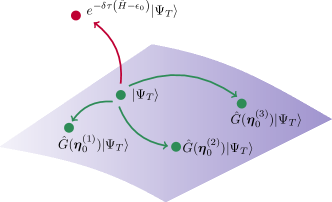
Figure 1: (color online) pictorial representation of the random walk in the manifold of $N$-particle Slater determinants $\mathfrak{D}(N)$ (lavender surface). The figure points out that the imaginary time propagator $e^{-\delta\tau\left(\hat{H}-\epsilon_{0}\right)}$ drives a Slater determinant $|\Psi_{T}\rangle$ away from $\mathfrak{D}(N)$, while the one-body propagators $\hat{G}({\mathbf{\eta}})$ preserve $\mathfrak{D}(N)$. This permits to retrieve the analytically intractable state $e^{-\delta\tau\left(\hat{H}-\epsilon_{0}\right)}|\Psi_{T}\rangle$ as a stochastic linear combination of Slater determinants $\hat{G}({\mathbf{\eta}}^{(w)}_{0})|\Psi_{T}\rangle$ according to (15).

Subsequently, each walker is let evolve under the action of the operators (10) and its weight is updated through multiplication by (8). An estimate for the ground state of the system is provided by the following stochastic linear combination of Slater determinants:

$$|\Phi_{0}\rangle\simeq\frac{1}{\sum_{w=1}^{N_{w}}\mathfrak{W}^{(w)}_{n}}\sum_{w=1}^{N_{w}}\mathfrak{W}^{(w)}_{n}\frac{|\Psi^{(w)}_{n}\rangle}{\langle\Psi_{T}|\Psi^{(w)}_{n}\rangle}$$ (15)

Since numeric calculations can be carried out on finitely-generated Hilbert spaces only, the numeric implementation of the phaseless AFQMC algorithm requires the single-particle Hilbert space basis (2) of the system to be truncated, i.e. only the $M$ lowest-energy plane-waves to be retained.

II.5 Dynamical Correlation Functions

The formalism outlined in II.2, II.4 enables the calculation of ground state properties, and also of the imaginary time correlation function (ITCF):

$$\begin{split}F_{\hat{A},\hat{B}}(\tau)&=\langle\Phi_{0}|\hat{A}e^{-\tau\left(\hat{H}-\epsilon_{0}\right)}\hat{B}|\Phi_{0}\rangle\\ \end{split}$$ (16)

of two single-particle many-body operators $\hat{A},\hat{B}$. (16) is a purely mathematical function, related to the dynamical or energy-resolved structure factor:

$$S_{\hat{A},\hat{B}}(\omega)=\int_{\mathbb{R}}dt\,\frac{e^{i\omega t}}{2\pi}\,\langle\Phi_{0}|\hat{A}(t)\hat{B}|\Phi_{0}\rangle$$ (17)

of $\hat{A},\hat{B}$, a quantity appearing in linear response theory and providing precious information on the time-dependent response of the system to external fields. Dynamical structure factors and ITCFs are related to each other, as revealed by their Lehmann representation, by a Laplace transform fetter .

Within the AFQMC formalism, the issue of computing ITCFs is complicated by the circumstance that the one-body operators $\hat{A},\hat{B}$ do not map Slater determinants onto Slater determinants, but on rather complicated states. Nevertheless, making use of the canonical anticommutation relations between fermionic creation and destruction operators it is possible to show noi that:

$$e^{-\delta\tau\left(\hat{H}-\epsilon_{0}\right)}\hat{B}=\int dg(\bm{\eta})\,\hat{B}(\bm{\eta})\hat{G}(\bm{\eta})$$ (18)

where $\hat{B}(\bm{\eta})$ is a suitable one-particle operator. In the case of the 2D HEG, it reads:

$$\begin{split}\hat{B}(\bm{\eta})&=\sum_{\bm{k}\bm{p}\sigma}\left(\mathcal{B}(\bm{\eta})\right)_{\bm{k}\bm{p}}\,\hat{a}^{\dagger}_{\bm{k}\sigma}\hat{a}_{\bm{p}\sigma}\end{split}$$ (19)

where:

$$\mathcal{B}(\bm{\eta})=\mathcal{D}(\bm{\eta})\mathcal{B}\mathcal{D}(\bm{\eta})^{-1}$$ (20)

is defined through:

$$\begin{split}\left(\mathcal{D}(\bm{\eta})\right)_{\bm{k}\bm{p}}=e^{-\frac{\delta\tau}{2}\left(\mathcal{H}_{0}\right)_{\bm{k}}}\left(e^{-i\sqrt{\delta\tau}\sum_{\bm{q}s}\eta_{\bm{q}s}\mathcal{A}_{s}(\bm{q})}\right)_{\bm{k}\bm{p}}e^{-\frac{\delta\tau}{2}\left(\mathcal{H}_{0}\right)_{\bm{p}}}\end{split}$$ (21)

By application of (18) and of the backpropagation technique shiwei_bp ; shiwei_bp2 ; noi , it is possible to express the ITCF $F_{\hat{A},\hat{B}}(\tau)$ as mean value of a random variable over the random path followed by the walkers in the manifold of Slater determinants.

Further details of this calculation procedure are reported in noi . For the purpose of the present work, it is sufficient to recall that the phaseless AFQMC estimator of $F_{\hat{A},\hat{B}}(\tau)$ reads:

$$\begin{split}F_{\hat{A},\hat{B}}(r\delta\tau)\simeq&\frac{1}{\sum_{w=1}^{N_{w}}\mathfrak{W}^{(w)}_{m+n-r}}\\ &\sum_{w=1}^{N_{w}}\sum_{ijkl}\,\mathcal{B}_{kl}\,\mathfrak{W}^{(w)}_{m+n}\,\frac{\langle\Psi^{(w)}_{BP,m}|\hat{A}\hat{a}^{\dagger}_{i}\hat{a}_{j}|\Psi^{(w)}_{n}\rangle}{\langle\Psi^{(w)}_{BP,m}|\Psi^{(w)}_{n}\rangle}\\ &\mathcal{D}(\bm{\eta}^{(w)}_{n-1}-\bm{\xi}^{(w)}_{n-1},\dots,\bm{\eta}^{(w)}_{n-r}-\bm{\xi}^{(w)}_{n-r})_{ik}\\ &\mathcal{D}^{-1}(\bm{\eta}^{(w)}_{n-1}-\bm{\xi}^{(w)}_{n-1},\dots,\bm{\eta}^{(w)}_{n-r}-\bm{\xi}^{(w)}_{n-r})_{lj}\\ \end{split}$$ (22)

where:

$$\begin{split}|\Psi^{(w)}_{BP,m}\rangle&=\hat{G}^{\dagger}(\bm{\eta}_{n}-\bm{\xi}_{n})\dots\hat{G}^{\dagger}(\bm{\eta}_{n+m-1}-\bm{\xi}_{n+m-1})|\Psi_{T}\rangle\\ \end{split}$$ (23)

and:

$$\begin{split}&\mathcal{D}(\bm{\eta}^{(w)}_{n-1}-\bm{\xi}^{(w)}_{n-1},\dots,\bm{\eta}^{(w)}_{n-r}-\bm{\xi}^{(w)}_{n-r})=\\ =&\mathcal{D}(\bm{\eta}^{(w)}_{n-1}-\bm{\xi}^{(w)}_{n-1})\dots\mathcal{D}(\bm{\eta}^{(w)}_{n-r}-\bm{\xi}^{(w)}_{n-r})\end{split}$$ (24)

The estimator (22) is essentially a weighted average of suitably-constructed matrix elements; each walker $w$ constructs the matrix element and the weights $\mathfrak{W}^{(w)}_{m+n-r}$, $\mathfrak{W}^{(w)}_{m+n}$ involved in the weighted average (22) from two Slater determinants $|\Psi^{(w)}_{n}\rangle$, $|\Psi^{(w)}_{BP,m}\rangle$ and two matrices $\mathcal{D}(\bm{\eta}^{(w)}_{n-1}-\bm{\xi}^{(w)}_{n-1},\dots,\bm{\eta}^{(w)}_{n-r}-\bm{\xi}^{(w)}_{n-r})$ These objects are functions of the auxiliary fields configurations $\bm{\eta}^{(w)}$ defining the random path followed by the walker in the manifold of Slater determinants, and their calculation is pictorially illustrated in Fig. 2.

Figure 2: (color online) pictorial representation of the phaseless AFQMC estimator for $F_{\hat{A},\hat{B}}(\tau)$, equation (22); $F_{\hat{A},\hat{B}}(\tau)$ is computed at $\tau=r\,\delta\tau$ with $r=2$, with $n=5$ propagation steps and $m=3$ backpropagation steps. The matrix $\mathcal{D}$ appearing in (24) is computed between the time steps $n-r$ and $n$ (at which $|\Psi^{(w)}_{n}\rangle$ is computed); the determinant $|\Psi^{(w)}_{BP,m}\rangle$ is computed between the time steps $n$ and $n+m$, and the weights $\mathfrak{W}^{(w)}_{m+n-r}$ and $\mathfrak{W}^{(w)}_{m+n}$ are computed at the time steps $m+n-r$ and $m+n$.

In the present work, we consider the imaginary time density-density correlation function:

$$F({\bm{q}},\tau)=\frac{\langle\Phi_{0}|\hat{\rho}_{-\bm{q}}e^{-\tau\left(\hat{H}-\epsilon_{0}\right)}\hat{\rho}_{\bm{q}}|\Phi_{0}\rangle}{N}$$ (25)

which is the Laplace transform of the dynamical structure factor $S(\bm{q},\omega)$. This quantity is notoriously related to the differential cross section of electromagnetic radiation scattering, and provides essential information for the quantitative description of excitations of the HEG, collective charge density flutuations, i.e. plasmons, end electron-hole excitations fetter ; vignale .

II.6 Numeric Stabilization

In a previous work noi we have pointed out that, due to the presence of such matrix elements, the estimator (22) is negatively-conditioned by a form of numeric instability. The aim of the present section is to elucidate the origin of such phenomenon and to propose a method for stabilizing the calculation of ITCFs in AFQMC. The AFQMC estimator (22) of the ITCF $F_{\hat{A},\hat{B}}(\tau)$ involves a weighted average, over the random paths followed by the $N_{w}$ walkers employed in the simulation, of a quantity in which the matrix elements of $\mathcal{D}(\bm{\eta}^{(w)}_{n-1}-\bm{\xi}^{(w)}_{n-1},\dots,\bm{\eta}^{(w)}_{n-r}-\bm{\xi}^{(w)}_{n-r})$ and of its inverse appear. In the reminder of the present section, these matrices will be referred to as $\mathcal{D}$ and $\mathcal{D}^{-1}$ for brevity. The matrices $\mathcal{D}$ and $\mathcal{D}^{-1}$ need to be computed numerically, respectively as product of $r$ matrices and inverse of $\mathcal{D}$. It is well-known that the numerical computation of $\mathcal{D}$ and $\mathcal{D}^{-1}$ introduces rounding-off errors Turing1948 , which accumulate as $r$ increases with detrimental impact on the results of the computation loh .

Rounding-off errors are particularly severe when the $\infty$-norm condition number:

$$\kappa(\mathcal{D})=\|\mathcal{D}\|_{\infty}\|\mathcal{D}^{-1}\|_{\infty}$$ (26)

of the matrix $\mathcal{D}$, in which $\|A\|_{\infty}=\max_{ij}|A_{ij}|$ denotes the $\infty$-norm on the space of $M\times M$ complex-valued matrices, is large. For the systems under study, we observe a condition number roughly increasing as $\kappa(\mathcal{D})\simeq C_{1}^{r}$ for some constant $C_{1}$. The rapid increase of $\kappa(\mathcal{D})$ indicates that the numeric matrix inversion $\mathcal{I}\left(\mathcal{D}\right)$ used to estimate $\mathcal{D}^{-1}$ might be ill-conditioned, an intuition that can be confirmed by studying the figure of merit:

$$\|E\|_{\infty}=\|\mathbb{I}-\mathcal{D}\mathcal{I}\left(\mathcal{D}\right)\|_{\infty}$$ (27)

For small $r$, $\frac{\|E\|_{\infty}}{M}$ is comparable with the machine precision $\epsilon=10^{-16}$; it then increases as $C_{2}^{r}$ for some constant $C_{2}$ and eventually saturates around $1$. In appendix (B) a qualitative explanation of the power-law increase of $\frac{\|E\|_{\infty}}{M}$ is provided. The gradual corruption of data revealed by the increase of $\|E\|_{\infty}$ reflects, as illustrated in figure (3), on the quality of the AFQMC estimates of ITCFs, which combine the matrix elements of $\mathcal{D}$ and $\mathcal{I}\left(\mathcal{D}\right)$ as prescribed by (22). We propose to mitigate the numeric instability of the ITCF estimator by performing a Tikhonov regularization Tikhonov1977 of the numeric inverse $\mathcal{I}\left(\mathcal{D}\right)$. Practically, the SVD of $\mathcal{D}$ is computed:

$$\mathcal{D}=U\mbox{diag}(\sigma_{1}\dots\sigma_{M})V^{\dagger}$$ (28)

and $\mathcal{I}\left(\mathcal{D}\right)$ is obtained as:

$$\mathcal{I}\left(\mathcal{D}\right)=V\mbox{diag}(\tilde{\sigma}_{1}\dots\tilde{\sigma}_{M})U^{\dagger}$$ (29)

where $\tilde{\sigma}_{i}=\frac{\sigma_{i}}{\lambda^{2}+\sigma_{i}^{2}}$ is defined by a regularization parameter $\lambda$. Large singular values $\sigma_{i}\gg\lambda$ are mapped to $\tilde{\sigma}_{i}\simeq\frac{1}{\sigma_{i}}$, while small singular values $\sigma_{i}\lesssim\lambda$ are kept below the threshold $\frac{1}{2\lambda}$. Particular care must be taken in choosing the regularization parameter $\lambda$, since for small $\lambda$ the Tikhonov regularization is clearly ineffective, while for large $\lambda$ it provokes a severe alteration in $\mathcal{I}\left(\mathcal{D}\right)$. On the other hand, an intermediate value of $\lambda$ prevents small errors in $\mathcal{D}$, associated to small singular values $\sigma_{i}$, to be dramatically amplified by the numeric inversion.

The effect of the Tikhonov regularization has been probed considering the model systems of $2$ particles introduced in noi , for which exact numeric solution of the Hamiltonian eigenvalue problem is feasible, and thus the ITCFs is exactly known. In figure (3) we show the effect of the Tikhonov regularization (29) on the ITCFs. The results show the existence of a broad interval of $\lambda$, comprising the machine precision $\epsilon=10^{-16}$, for which the Tikhonov regularization mitigates the numeric instability affecting the AFQMC estimator of ITCFs without introducing any appreciable bias besides that introduced by the real local energy and phaseless approximations. The figure displays, in the upper and lower panel respectively, the statistical errors of the AFQMC estimations and the discrepancies with respect to the exact results for three different values of $\lambda$. It is evident that, as the imaginary time becomes large, the effect of the regularization is very important.

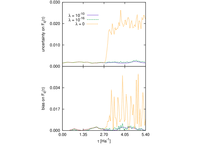
Figure 3: (color online) Effect of the Tykhonoff regularization (29) on an ITCFs relative to a system of $N=2$ electrons with $M=21$ basis set elements. Upper panel: statistical uncertainty affecting the AFQMC estimate of $F(q,\tau)$ with $\lambda=10^{-10}$ (lavender solid lines), $\lambda=10^{-16}$ (green dashed lines) and $\lambda=0$ (orange dotted lines). Lower panel: bias affecting the AFQMC estimate of $F(q,\tau)$.

II.7 Computational Cost

The AFQMC estimator of ITCFs should join numeric stability and low computational cost. The aim of the present section is to show that the computational cost of (22) is $\mathcal{O}(M^{3})$, $M$ being the number of orbitals constituting the single-particle basis. The contribution $F_{w}$ to (22) brought by a single walker of index $w$ reads:

$$\begin{split}F_{w}=\sum_{ijklrs}\mathcal{A}_{rs}\,\mathcal{B}_{kl}\,\langle\hat{a}^{\dagger}_{r}\hat{a}_{s}\hat{a}^{\dagger}_{i}\hat{a}_{j}\rangle_{w}\mathcal{D}_{ik}\mathcal{D}^{-1}_{lj}\\ \end{split}$$ (30)

where the abbreviation:

$$\langle\cdot\rangle_{w}=\frac{\langle\Psi^{(w)}_{BP,m}|\cdot|\Psi^{(w)}_{n}\rangle}{\langle\Psi^{(w)}_{BP,m}|\Psi^{(w)}_{n}\rangle}$$ (31)

has been inserted. The generalized Wick’s theorem balian ; noi implies that:

$$\langle\hat{a}^{\dagger}_{r}\hat{a}_{s}\hat{a}^{\dagger}_{i}\hat{a}_{j}\rangle_{w}=\langle\hat{a}^{\dagger}_{r}\hat{a}_{s}\rangle_{w}\langle\hat{a}^{\dagger}_{i}\hat{a}_{j}\rangle_{w}+\langle\hat{a}^{\dagger}_{r}\hat{a}_{j}\rangle_{w}\langle\hat{a}_{s}\hat{a}^{\dagger}_{i}\rangle_{w}$$ (32)

(32) is most conveniently expressed, introducing the definition $\mathcal{G}_{ij}=\langle\hat{a}^{\dagger}_{i}\hat{a}_{j}\rangle_{w}$ and recalling canonical anticommutation relations, as:

$$\langle\hat{a}^{\dagger}_{r}\hat{a}_{s}\hat{a}^{\dagger}_{i}\hat{a}_{j}\rangle_{w}=\mathcal{G}_{rs}\mathcal{G}_{ij}+\mathcal{G}_{rj}\left(\delta_{is}-\mathcal{G}_{is}\right)$$ (33)

Combining (30) and (33) yields:

$$\begin{split}F_{w}&=\sum_{ijklrs}\mathcal{A}_{rs}\,\mathcal{B}_{kl}\,\mathcal{G}_{rs}\mathcal{G}_{ij}\mathcal{D}_{ik}\mathcal{D}^{-1}_{lj}\\ &+\sum_{ijklr}\mathcal{A}_{ri}\,\mathcal{B}_{kl}\,\mathcal{G}_{rj}\mathcal{D}_{ik}\mathcal{D}^{-1}_{lj}\\ &-\sum_{ijklrs}\mathcal{A}_{rs}\,\mathcal{B}_{kl}\,\mathcal{G}_{rj}\mathcal{G}_{is}\mathcal{D}_{ik}\mathcal{D}^{-1}_{lj}\\ \end{split}$$ (34)

Despite its cumbersome appearance, (34) can be efficiently evaluated computing the intermediate tensors $\mathcal{D}\mathcal{B}$, $\mathcal{A}\mathcal{G}^{T}$ and $\mathcal{D}^{-1}\mathcal{G}^{T}$ at the cost of $\mathcal{O}(M^{3})$ operations, and subsequently computing $F_{w}$ as:

$$\begin{split}F_{w}&=\left(\sum_{r}\left(\mathcal{A}\mathcal{G}^{T}\right)_{rr}\right)\left(\sum_{il}\left(\mathcal{D}\mathcal{B}\right)_{il}\left(\mathcal{D}^{-1}\mathcal{G}^{T}\right)_{li}\right)\\ &+\sum_{ilr}\left(\mathcal{D}\mathcal{B}\right)_{il}\left(\mathcal{D}^{-1}\mathcal{G}^{T}\right)_{lr}\mathcal{A}_{ri}\\ &-\sum_{ilr}\left(\mathcal{D}\mathcal{B}\right)_{il}\left(\mathcal{D}^{-1}\mathcal{G}^{T}\right)_{li}\left(\mathcal{A}\mathcal{G}^{T}\right)_{ri}\end{split}$$ (35)

at the cost of $\mathcal{O}(M^{3})$ more operations. The calculation of $F_{w}$ further simplifies for operators $\hat{A}$ whose matrix elements read $\mathcal{A}_{ij}=\mathcal{A}_{j}\,\delta_{i,a(j)}$ for some function $a:\{1\dots M\}\to\{1\dots M\}$. The density fluctuation operator $\hat{\rho}_{\bm{q}}=\sum_{\bm{k}\sigma}\hat{a}^{\dagger}_{\bm{k}+\bm{q}\sigma}\hat{a}_{\bm{k}\sigma}$ falls within such category.

The complexity $\mathcal{O}(M^{3})$ is the best allowed by the phaseless AFQMC methodology: in fact, the calculation of ITCFs requires at least $\mathcal{O}(M^{3})$ operations to accumulate the matrix $\mathcal{D}$, and the contractions in (34) do not compromise this favorable scaling with the number of single-particle orbitals.

III Results

In the present work we have simulated paramagnetic systems of $N=18,26,42$ electrons at $r_{s}=0.1,0.5,1$; we show also results for $N=18$ particles at $r_{s}=2$. Our calculations qualify the phaseless AFQMC as a practical and useful methodology for the accurate evaluation of $F(\bm{q},\tau)$, for systems of $N=\mathcal{O}(10^{2})$ correlated fermions in the continuum. The complexity scales as $M^{3}$ ($M$ being the number of basis sets elements), and the absolute statistical error of $F(\bm{q},\tau)$ can be kept at the level $10^{-3}-2.5\,10^{-3}$ with moderate computational resources even at values of $\tau\simeq 3/E_{F}$ for $r_{s}=0.1,0.5,1$ and $\tau\simeq 2.5/E_{F}$ for $r_{s}=2$, $E_{F}=1/r_{s}^{2}$ being the Fermi energy.

The number $N$ of electrons constituting the system is inferior to that typically involved in QMC ground state calculations of bulk fermionic systems, but comparable to that used in the context of excited-states calculations through imaginary time correlation functions evaluated via configurational QMC methods reported in literaturefc .

The imaginary time steps used in our calculations were $\delta\tau=0.003,0.004,0.006,0.008$ $E_{Ha}^{-1}$ at $r_{s}=0.1,0.5,1,2$ respectively. For each simulation, the number of plane-waves constituting the single-particle Hilbert space has been raised up to $M=300$ according to the number of particles and to the strength of the interaction. For all calculations, it was verified that decreasing the time step and increasing the number of plane-waves had a negligible effect on the ground state energy. To obtain correct estimates of ITCFs, it is necessary to perform a sufficiently large number $m$ of backpropagation steps. However, it is well-known shiwei_bp2 that raising $m$ can result in an increase in variance, which severely limits the possibility of extracting physical information from the long imaginary-time tails of the ITCFs. We have used a number of backpropagation steps in the range $m=200-600$. When $m=600$ has proved insufficient, to avoid the increases in variance mentioned above, AFQMC estimates have been extrapolated to the $m\to\infty$ limit (data obtained by extrapolation will be henceforth marked with an asterisk).

III.1 Imaginary time correlation functions and excitation energies

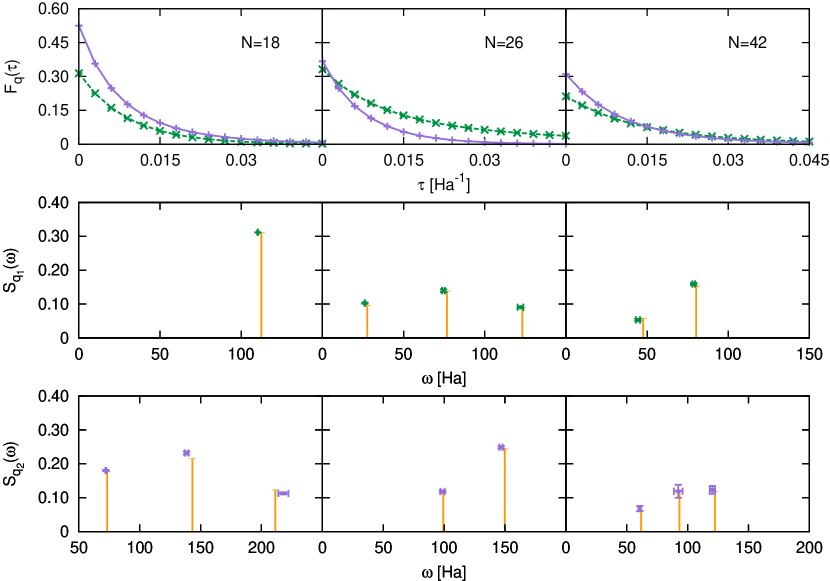
Figure 4: (color online) Upper panel: imaginary time correlation functions of the density fluctuation operator $\hat{\rho}_{\bm{q}}$ for paramagnetic systems of $N=18,26$ and $42$ particles (left to right) at $r_{s}=0.1$, with transferred momenta $\bm{q}_{1}$ (green dashed lines) and $\bm{q}_{2}$ (lavender solid lines). When not visible, errors are below the symbol size. Lines are only a guide for eyes. Central panel: dynamical structure factor for $N=18,26$ and $42$ particles (left to right) with transferred momentum $\bm{q}_{1}$ (RPA: orange impulses, AFQMC: green symbols). Lower panel: dynamical structure factor for $N=18,26$ and $42$ particles (left to right) with transferred momentum $\bm{q}_{2}$ (RPA: orange impulses, AFQMC: lavender symbols).

For all the values of $N$ and $r_{s}$, an AFQMC estimate of the ITCF (25) is produced according to the procedure sketched in section II.5. The obtained $F(\bm{q},\tau)$ is shown in the upper panel of Figures 4, 5, 6 and 7. As it is well-known gift , it is highly non-trivial to extract physical information from ITCFs. In the case of the HEG, the finite size of the systems under study induces to expect contributions to $F(\bm{q},\tau)$ coming from excited states of the system, which are obtained from the ground state by creation of particle-hole pairs. The dynamical structure factor $S(\bm{q},\omega)$, the inverse Laplace transform of $F(\bm{q},\tau)$, is thus expected to display multiple peaks corresponding to the excitation energies. This picture is confirmed by RPA calculations for finite systems, reported in Appendix C.

The presence of multiple peaks complicates the task of performing the analytic continuation providing an estimation of $S(\bm{q},\omega)$. Therefore, since the number of peaks grows rapidly with the wave-vector modulus $|\bm{q}|$, we have limited our attention to the wave-vectors $\bm{q}_{1}=(2\pi/L)\,(1,0)$ and $\bm{q}_{2}=(2\pi/L)\,(1,1)$. Notice that $|\bm{q}_{1}|/k_{F}=0.707,0.5,0.447$ and $|\bm{q}_{2}|/k_{F}=1,0.707,0.632$ for $N=18,26,42$ respectively. Naturally, $k_{F}=\sqrt{2}/r_{s}$ is the Fermi wave-vector. These low-momentum excitations are very interesting also from a physical point of view, in connection with the well-known collective plasmon excitation of the HEG. Therefore, we do not attempt to predict the full $S(\bm{q},\omega)$, but limit ourselves to extract the excitations energies and weights by fitting the evaluated ITCF to a sum:

$$F(\tau)=\sum_{i=1}^{N_{w}}s_{i}e^{-\tau\omega_{i}}$$ (36)

of exponential functions with positive frequencies $\omega_{i}$ and weights $s_{i}$ relying on the well-established Levenberg-Marquardt curve-fitting method Levenberg1944 . The number $N_{w}\leq 3$ of such frequencies and weights is that leading to the best fit.

In Figures 4, 5, 6 and 7 we show results relative to the simulation of paramagnetic systems at $r_{s}=0.1,0.5,1,2$ respectively. Each figure contains data relative to the particle numbers $N=18,26,42$ and wave-vectors $\bm{q}_{1},\bm{q}_{2}$. In the upper panel we show the estimated $F(\bm{q},\tau)$, while in the middle and lower panels we show, for $\bm{q}_{1}$ and $\bm{q}_{2}$ respectively, the obtained frequencies and weights, together with the RPA results. The AFQMC estimations of the quantities $s_{i},\omega_{i}$ are displayed as points with both horizontal and vertical statistical errors: the horizontal ones provide the uncertainties on the frequencies $\omega_{i}$ of the excitations, while the vertical ones gives the error bars on the weights $s_{i}$. The coordinates of the points give, naturally, the mean frequencies and weights. The statistical uncertainties on the quantities $s_{i},\omega_{i}$ are those yield by the fit procedure. The frequencies predicted by the RPA are represented as impulses with height equal to the corresponding weights. We see that, at $r_{s}=0.1$, there is a close agreement between AFQMC and RPA predictions of both frequencies and spectral weights. Since it is known that, for small $r_{s}$, RPA predictions are very accurate, such agreement provides a robust check for the reliability of AFQMC methodology in providing information about the manifold of excited states of the system. It is well known noi that, in the same situation, calculations of $F(\bm{q},\tau)$ based on the Fixed-Node approximation would give inaccurate results even if the nodal structure of the ground state wave function is known with very high accuracy. As $r_{s}$ increases, discrepancies appear between the two approaches. The presence of such discrepancies is naturally expected: none of the methodologies used in the present work is free from approximations. The approximations underlying RPA and AFQMC, in particular, are quite different in nature and are expected to agree only in the limit of high density (very low $r_{s}$). Incidentally, we observe that, due to the finite size of the systems investigated, we cannot provide quantitative predictions about the plasmonic mode, which becomes a well defined collective excitation in the thermodynamic limit. What we expect is that, as the system size becomes large enough, of the several peaks that are present for the finite systems, one will acquire a dominant spectral weight, eventually becoming a well defined collective excitation. In order to further assess the quality of our results, in Tables 1, 2 and 3 we detail the comparison with the RPA and configurational Monte Carlo results for the ground state energy per particle, the static structure factor $S(\bm{q})=F(\bm{q},0)$ and the static density response function:

$$\tilde{\chi}(\bm{q})=-\frac{\chi(\bm{q})}{2n}=\int_{0}^{+\infty}d\tau\,F(\bm{q},\tau)$$ (37)

In the AFQMC calculations, $\tilde{\chi}(\bm{q})$ is obtained using the parameters yield by the fitting procedure of the density-density correlations $F(\bm{q},\tau)$. As far as ground state energies per particle are concerned, as shown in Table 1, at $r_{s}=0.1$ the three methods give compatible results. As $r_{s}$ increases, AFQMC estimates are always closer to FN than RPA, lying between them. The configurational Quantum Monte Carlo evaluation of the ground state per particle has been obtained via Diffusion Quantum Monte Carlo (DMC) calculation, with a nodal structure encompassing backflow correlations, optimized by means of the Linear Method Umrigar2008 ; Motta2015 . It is well-known that FN calculations with optimized nodal structures yield highly accurate estimates of the ground state energy, as confirmed by comparison with Full Configuration Interaction QMC calculations Alavi2012 ; Alavi2013 : this result, therefore, confirms the great accuracy of the phaseless approximation phaseless1 ; phaseless2 .

The configurational QMC evaluation of the static structure factor $S(\bm{q})$ has been obtained via FN DMC calculations with the nodal structure described above. DMC estimates have been extrapolated Foulkes2001 . Moreover, we have compared AFQMC estimations of the static density response function $\tilde{\chi}(\bm{q})$ with RPA and Fixed-Node estimations. In principle, the Fixed-Node evaluation of the static density response function $\tilde{\chi}(\bm{q})$ is highly non trivial, involving the manifold of excited states. However, it is well-known that this difficulty can be circumvented saverio1 extracting $\tilde{\chi}(\bm{q})$ from the ground state energy $E(v_{\bm{q}})$ of a system subject to an external periodic potential of amplitude $v_{\bm{q}}$ in the $v_{\bm{q}}\to 0$ limit. We observe that, increasing $r_{s}$ above $0.1$, the AFQMC predictions remain, in general, closer to the configurational Monte Carlo ones than to the RPA ones: this is a strong indication about the quality of AFQMC results, since the Monte Carlo calculations include correlations beyond the RPA level. This result is remarkable, since the AFQMC evaluation of $\tilde{\chi}(\bm{q})$ is considerably influenced by the low-energy excitations which, if predicted unaccurately, can significantly bias the result. As $r_{s}$ further increases, however, the agreement decreases. We have verified that the number of plane-waves and the number of backpropagation steps are sufficiently large to extrapolate the results and to filter the excited states contributions from the trial wave function. Hence, the origin of the discrepancies between the estimations yield by the three methodologies used in the present work has to be sought in the approximation schemes underlying them.

$N$	$r_{s}$	$\frac{\epsilon_{0}}{N}$ (RPA)	$\frac{\epsilon_{0}}{N}$ (AF)	$\frac{\epsilon_{0}}{N}$ (FN)
18	0.1	40.14	40.14(2)	40.13(1)
26	0.1	45.84	45.82(1)	45.81(1)
42	0.1	42.18	42.18(1)	42.17(1)
18	0.5	0.5065	0.5007(2)	0.5012(2)
26	0.5	0.7520	0.7360(2)	0.7326(8)
42	0.5	0.6031	0.6002(1)	0.5922(9)
18	1.0	-0.2489	-0.2562(1)	-0.2580(1)
26	1.0	-0.1847	-0.1921(1)	-0.1961(1)
42	1.0	-0.2215	-0.2283(1)	-0.2309(2)
18	2.0	-0.2661	-0.2695(1)	-0.2717(1)

Table 1: RPA (column 3), AFQMC (column 4) and FN-DMC (column 5) estimates of the ground state energy for various systems (parameters are listed in columns 1-3); energies are measured in $E_{Ha}$. The RPA ground state energy is calculated on the Gaskell trial wavefunction Gaskell1962 .

$N$	$r_{s}$	$|\bm{q}|$	$S(\bm{q})$ (RPA)	$S(\bm{q})$ (AF)	$S(\bm{q})$ (FN)
18	0.1	8.355427	0.3105	0.314(2)	0.319(4)
18	0.1	11.81636	0.5150	0.525(4)	0.521(4)
26	0.1	6.952136	0.3326	0.342(2)	0.343(4)
26	0.1	9.831805	0.3623	0.367(6)	0.370(5)
42	0.1	5.469911	0.2101	0.212(7)	0.217(4)
42	0.1	7.735622	0.3045	0.310(6)	0.306(5)
18	0.5	1.671085	0.2511	0.258(1)	0.266(4)
18	0.5	2.363271	0.4137	0.440(3)	0.448(5)
26	0.5	1.390427	0.2225	0.254(3)∗	0.238(4)
26	0.5	1.966361	0.3009	0.313(2)	0.322(4)
42	0.5	1.093982	0.1533	0.161(2)	0.146(5)
42	0.5	1.547124	0.2366	0.247(2)	0.264(4)
18	1.0	0.835543	0.2098	0.231(2)	0.218(5)
18	1.0	1.181636	0.3451	0.395(3)	0.386(4)
26	1.0	0.695214	0.1746	0.227(2)∗	0.192(5)
26	1.0	0.983181	0.2558	0.289(2)	0.281(4)
42	1.0	0.546991	0.1219	0.141(1)	0.126(5)
42	1.0	0.773562	0.1938	0.219(2)	0.208(5)
18	2.0	0.417771	0.1657	0.172(2)∗	0.176(4)
18	2.0	0.590818	0.2732	0.304(3)∗	0.305(4)

Table 2: RPA (column 4), AFQMC (column 5) and FN-DMC (column 6) estimates of the static structure factor $S(\bm{q})$ for various systems and wave-vectors (parameters are listed in columns 1-3); wave-vectors are measured in $a_{B}^{-1}$. AFQMC estimates marked with an asterisk are extrapolated.

$N$	$r_{s}$	$|\bm{q}|$	$\tilde{\chi}(\bm{q})$ (RPA)	$\tilde{\chi}(\bm{q})$ (AF)	$\tilde{\chi}(\bm{q})$ (FN)
18	0.1	8.355427	0.00276	0.0028(4)	0.00287(1)
18	0.1	11.81636	0.00449	0.0046(1)	0.00469(1)
26	0.1	6.952136	0.00598	0.0065(2)	0.00653(4)
26	0.1	9.831805	0.00282	0.0028(1)	0.00287(4)
42	0.1	5.469911	0.00311	0.0032(4)	0.00325(4)
42	0.1	7.735622	0.00330	0.0034(2)	0.00335(2)
18	0.5	1.671085	0.04516	0.048(1)	0.0484(4)
18	0.5	2.363271	0.06992	0.081(2)	0.0788(4)
26	0.5	1.390427	0.06298	0.085(6)∗	0.069(2)
26	0.5	1.966361	0.04827	0.051(1)	0.0504(4)
42	0.5	1.093982	0.04074	0.043(5)	0.042(2)
42	0.5	1.547124	0.04903	0.051(3)	0.049(2)
18	1.0	0.835543	0.12612	0.152(3)	0.143(2)
18	1.0	1.181636	0.18979	0.301(6)	0.226(1)
26	1.0	0.695214	0.14601	0.22(2)∗	0.162(2)
26	1.0	0.983181	0.13872	0.188(6)	0.161(2)
42	1.0	0.546991	0.10212	0.158(7)	0.14(1)
42	1.0	0.773562	0.13014	0.176(9)	0.16(1)
18	2.0	0.417771	0.31451	0.34(1)∗	0.374(4)
18	2.0	0.590818	0.46238	0.89(1)∗	0.590(2)

Table 3: RPA (column 4), AFQMC (column 5) and FN-DMC (column 6) estimates of the compressibility $\tilde{\chi}(\bm{q})$ for various systems and wave-vectors (parameters are listed in columns 1-3); wave-vectors are measured in $a_{B}^{-1}$, and $\tilde{\chi}(\bm{q})$ in $E_{Ha}^{-1}$. AFQMC estimates marked with an asterisk are extrapolated.

$\mathrm{r_{s}}=0.1$

$\mathrm{r_{s}}=0.5$

Figure 5: (color online) Upper panel: imaginary time correlation functions of the density fluctuation operator $\hat{\rho}_{\bm{q}}$ for paramagnetic systems of $N=18,26$ and $42$ particles (left to right) at $r_{s}=0.5$, with transferred momenta $\bm{q}_{1}$ (green dashed lines) and $\bm{q}_{2}$ (lavender solid lines). When not visible, errors are below the symbol size. Lines are only a guide for eyes. Central panel: dynamical structure factor for $N=18,26$ and $42$ particles (left to right) with transferred momentum $\bm{q}_{1}$ (RPA: orange impulses, AFQMC: green symbols). Lower panel: dynamical structure factor for $N=18,26$ and $42$ particles (left to right) with transferred momentum $\bm{q}_{2}$ (RPA: orange impulses, AFQMC: lavender symbols).

$\mathrm{r_{s}}=1$

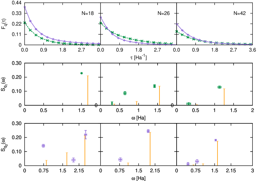
Figure 6: (color online) Upper panel: imaginary time correlation functions of the density fluctuation operator $\hat{\rho}_{\bm{q}}$ for paramagnetic systems of $N=18,26$ and $42$ particles (left to right) at $r_{s}=1$, with transferred momenta $\bm{q}_{1}$ (green dashed lines) and $\bm{q}_{2}$ (lavender solid lines). When not visible, errors are below the symbol size. Lines are only a guide for eyes. Central panel: dynamical structure factor for $N=18,26$ and $42$ particles (left to right) with transferred momentum $\bm{q}_{1}$ (RPA: orange impulses, AFQMC: green symbols). Lower panel: dynamical structure factor for $N=18,26$ and $42$ particles (left to right) with transferred momentum $\bm{q}_{2}$ (RPA: orange impulses, AFQMC: lavender symbols).

$\mathrm{r_{s}}=2$

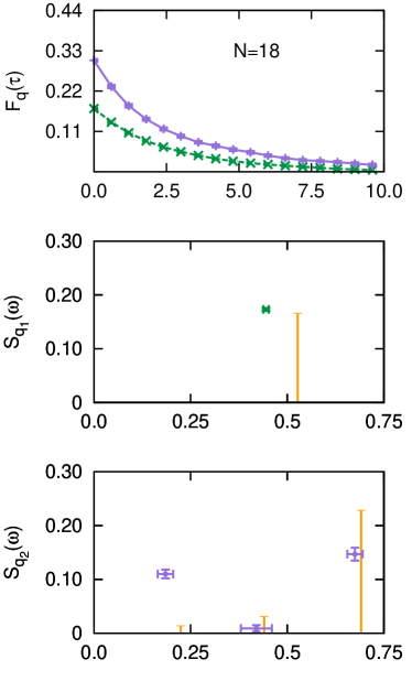
Figure 7: (color online) Upper panel: imaginary time correlation functions of the density fluctuation operator $\hat{\rho}_{\bm{q}}$ for paramagnetic systems of $N=18,26$ and $42$ particles (left to right) at $r_{s}=2$, with transferred momenta $\bm{q}_{1}$ (green dashed lines) and $\bm{q}_{2}$ (lavender solid lines). When not visible, errors are below the symbol size. Lines are only a guide for eyes. Central panel: dynamical structure factor for $N=18,26$ and $42$ particles (left to right) with transferred momentum $\bm{q}_{1}$ (RPA: orange impulses, AFQMC: green symbols). Lower panel: dynamical structure factor for $N=18,26$ and $42$ particles (left to right) with transferred momentum $\bm{q}_{2}$ (RPA: orange impulses, AFQMC: lavender symbols).

IV Conclusions

We have shown the possibility to provide accurate first principles calculations of imaginary time correlations for medium-sized fermionic systems in the continuum, using the phaseless Auxiliary Fields Quantum Monte Carlo method.

We have simulated a $2D$ homogeneous electron gas of up to $N=42$ electrons using a plane-waves basis set of up to $M=300$ elements. We have shown that the density-density correlation function in imaginary time can be calculated via a polynomially complex algorithm with the favorable scaling $\mathcal{O}(M^{3})$. In order to achieve a good accuracy level in the calculations, we propose stabilization procedures to deal with matrix inversion, which can be used in combination with well-established stabilization procedures for matrix exponentiation and multiplication Sugar ; Alhassid : in particular, we suggest a Tikhonov regularization that allows to maintain a good accuracy level even for imaginary time values of the order of $3/E_{F}$. We have yielded also comparisons with predictions of the static structure factor and the static density response obtained via the RPA approximation and via Fixed-Node Quantum Monte Carlo calculations.

At small $r_{s}$ the AFQMC correctly reproduces the RPA results. At larger $r_{s}$ on the other hand, it provides quantitative estimates of the deviations from the RPA, as the comparison with FN calculations reveals. We believe this is a relevant result for QMC simulations: it is known, in fact, that the widely employed Fixed-Node approximation fails to properly sample the imaginary-time propagator, due to the imposition of the ground-state nodal structure to excited states. AFQMC, on the other hand, appears to provide a useful tool to explore, from first principles, the manifold of the excited states of a fermionic system.

V Acknowledgements

We acknowledge the CINECA and the Regione Lombardia award, under the LISA initiative, for the availability of high-performance computing resources and support. M. M. also acknowledges funding provided by the Dr. Davide Colosimo Award, celebrating the memory of physicist Davide Colosimo.

Appendix A Hubbard-Stratonovich Transformation for the 2DHEG

By a straightforward application of the canonical anticommutation relations, the Hamiltonian (1) can be exactly rewritten as:

$$\hat{H}=\sum_{\bm{k}\sigma}\left(\frac{|\bm{k}|^{2}}{2}-\mu(\bm{k})\right)\,\hat{a}^{\dagger}_{\bm{k}\sigma}\hat{a}_{\bm{k}\sigma}+\frac{1}{2\Omega}\,\sum_{\bm{q}}\frac{2\pi}{|\bm{q}|}\hat{\rho}_{\bm{q}}\hat{\rho}_{-\bm{q}}$$ (38)

where:

$$\mu(\bm{k})=\frac{1}{2\Omega}\sum_{\bm{p}\neq\bm{k}}\frac{2\pi}{|\bm{p}-\bm{k}|}$$ (39)

and $\hat{\rho}_{\bm{q}}=\sum_{\bm{k}\sigma}\hat{a}^{\dagger}_{\bm{k}-\bm{q}\sigma}\hat{a}_{\bm{k}\sigma}$ is the density fluctuation operator. Recalling the parity of $\frac{2\pi}{|\bm{q}|}$ and the anticommutation relation:

$$\left[\hat{\rho}_{\bm{q}},\hat{\rho}_{-\bm{q}}\right]_{+}=\frac{(\hat{\rho}_{\bm{q}}+\hat{\rho}_{-\bm{q}})^{2}}{2}+\frac{(i\hat{\rho}_{\bm{q}}-i\hat{\rho}_{-\bm{q}})^{2}}{2}$$ (40)

one eventually finds:

$$\hat{H}=\hat{H}_{0}+\frac{1}{2}\,\sum_{\bm{q}}\left(\hat{A}_{1}(\bm{q})^{2}+\hat{A}_{2}(\bm{q})^{2}\right)$$ (41)

with:

$$\hat{H}_{0}=\sum_{\bm{k}\sigma}\left(\frac{|\bm{k}|^{2}}{2}-\mu(\bm{k})\right)\,\hat{a}^{\dagger}_{\bm{k}\sigma}\hat{a}_{\bm{k}\sigma}$$ (42)

and:

$$\hat{A}_{1}(\bm{q})=\sqrt{\frac{2\pi}{\Omega|\bm{q}|}}\,\frac{\hat{\rho}_{\bm{q}}+\hat{\rho}_{-\bm{q}}}{2}\quad\hat{A}_{2}(\bm{q})=\sqrt{\frac{2\pi}{\Omega|\bm{q}|}}\,\frac{i\hat{\rho}_{\bm{q}}-i\hat{\rho}_{-\bm{q}}}{2}$$ (43)

which, since $\hat{\rho}_{-\bm{q}}=\hat{\rho}_{\bm{q}}^{\dagger}$, are hermitian operators. Applying the Hubbard-Stratonovich transformation to the propagator of the Hamiltonian (11) yields:

$$\hat{G}(\bm{\eta})=e^{-\frac{\delta\tau}{2}\hat{H}_{0}}e^{-i\sqrt{\delta\tau}\sum_{\bm{q}}\eta_{1\bm{q}}\hat{A}_{1}(\bm{q})+\eta_{2\bm{q}}\hat{A}_{2}(\bm{q})}e^{-\frac{\delta\tau}{2}\hat{H}_{0}}$$ (44)

Appendix B Numeric Stability of Matrix Inversion

The distance:

$$\|\mathcal{I}\left(\mathcal{D}_{r}\right)-\mathcal{D}_{r}^{-1}\|_{\infty}$$ (45)

between the actual inverse $\mathcal{D}_{r}^{-1}$ of $\mathcal{D}_{r}$ and its numeric estimate $\mathcal{I}\left(\mathcal{D}_{r}\right)$ (45) is bounded Turing1948 by:

$$\|\mathcal{I}\left(\mathcal{D}_{r}\right)-\mathcal{D}_{r}^{-1}\|_{\infty}\leq M\|\mathcal{I}\left(\mathcal{D}_{r}\right)\|_{\infty}\frac{\|E_{r}\|_{\infty}}{1-M\|E_{r}\|_{\infty}}$$ (46)

with:

$$\|E_{r}\|_{\infty}=\|\mathbb{I}-\mathcal{D}_{r}\mathcal{I}\left(\mathcal{D}_{r}\right)\|_{\infty}$$ (47)

Equation (46) holds for $\|E_{r}\|_{\infty}<\frac{1}{M}$, and is therefore adequate to the description of $\|E_{r}\|_{\infty}$ for small $r$. It can be combined with the following estimate Fox1948 :

$$\|\mathcal{I}\left(\mathcal{D}_{r}\right)-\mathcal{D}_{r}^{-1}\|_{\infty}\simeq\epsilon\|\mathcal{D}_{r}^{-1}\|^{2}_{\infty}\frac{M^{3}}{3}$$ (48)

to yield:

$$M\|E_{r}\|_{\infty}\simeq\frac{\epsilon\frac{M^{3}}{3}\|\mathcal{D}_{r}^{-1}\|^{2}_{\infty}}{\|\mathcal{I}\left(\mathcal{D}_{r}\right)\|_{\infty}+\epsilon\frac{M^{3}}{3}\|\mathcal{D}_{r}^{-1}\|^{2}_{\infty}}$$ (49)

In the case of AFQMC calculations, where $\mathcal{D}_{r}$ and $\mathcal{D}_{r}^{-1}$ come from the product of $r$ matrices:

$$\|\mathcal{D}_{r}^{-1}\|_{\infty}=C_{3}^{r}\quad\|\mathcal{I}(\mathcal{D}_{r})\|_{\infty}=C_{4}^{r}$$ (50)

where $C_{3}$ and $C_{4}$ are suitable constants, close to each other. Merging (48) and (50) leads to:

$$\|E_{r}\|_{\infty}\simeq\frac{\epsilon\frac{M^{2}}{3}}{\left(\frac{C_{4}}{C_{3}^{2}}\right)^{r}+\epsilon\frac{M^{3}}{3}}$$ (51)

which reduces to:

$$\|E_{r}\|_{\infty}\simeq\epsilon\frac{M^{2}}{3}\left(\frac{C_{3}^{2}}{C_{4}}\right)^{r}$$ (52)

in the limit of small $r$. Since $C_{4}<C_{3}^{2}$, $C_{3}$ and $C_{4}$ being close to each other, the estimate (52) leads to a power-law increase of $\|E_{r}\|_{\infty}$.

Appendix C RPA for Finite Homogeneous Systems

The aim of this appendix is to provide a brief description of the Random Phase Approximation (RPA) Sawada1957 ; fetter ; vignale for finite interacting systems and of the procedure leading to the excitation energies and weights, with which AFQMC results have been compared.

The RPA can be regarded to fetter as a refinement of the well-known Tamm-Dancoff approximation tamm ; dancoff ; fetter (TDA), which has long been supporting the study of excitations in nuclear systems. The TDA relies on the assumptions that the ground state of the system is the Hartree-Fock determinant, and that excited states can be represented as superpositions of determinants obtained promoting a single particle above the Fermi surface. Within RPA, on the other hand, a better approximation $|\Phi_{0}\rangle$ for the actual ground state of the interacting system is employed to build up an Ansatz for plasmonic wavefunctions. To this purpose, the distinction between spin-orbitals below and above the Fermi level is made explicit by writing:

$$\hat{a}^{\dagger}_{\bm{k}\sigma}=\left\{\begin{split}\hat{c}^{\dagger}_{\bm{k}\sigma}\quad\mbox{if $|\bm{k}|>k_{F}$}\\ \hat{b}^{\phantom{{\dagger}}}_{\bm{k}\sigma}\quad\mbox{if $|\bm{k}|\leq k_{F}$}\\ \end{split}\right.$$ (53)

and the Hamiltonian (1) is consequently expressed as:

$$\begin{split}\hat{H}&=\hat{T}+\hat{V}=\\ &=\sum_{\bm{k}\sigma}t_{\bm{k}}\,\hat{c}^{{\dagger}}_{\bm{k}\sigma}\hat{c}^{\phantom{{\dagger}}}_{\bm{k}\sigma}+\sum_{\bm{k}\sigma}t_{\bm{k}}\,\left(1-\hat{b}^{\dagger}_{\bm{k}\sigma}\hat{b}^{\phantom{{\dagger}}}_{\bm{k}\sigma}\right)+\\ &+\frac{1}{2\Omega}\,\sum_{\bm{q}\neq 0}\phi_{\bm{q}}\hat{\rho}_{\bm{q}}\hat{\rho}_{-\bm{q}}\end{split}$$ (54)

where $t_{\bm{k}}=\frac{|\bm{k}|^{2}}{2}$, $\phi_{\bm{q}}=\frac{2\pi}{|\bm{q}|}$, the first sum goes over all wave-vectors $\bm{k}$ such that $|\bm{k}|>k_{F}$, the second sum goes over all wave-vectors $\bm{k}$ such that $|\bm{k}|\leq k_{F}$ and the density fluctuation operator $\hat{\rho}_{\bm{q}}$ is approximated Sawada1957 by:

$$\hat{\rho}_{\bm{q}}\simeq\sum_{\bm{k}\sigma}\hat{c}^{{\dagger}}_{\bm{k+q}\sigma}\hat{b}^{\dagger}_{\bm{k}\sigma}+\hat{b}^{\phantom{{\dagger}}}_{\bm{k+q}\sigma}\hat{c}^{\phantom{{\dagger}}}_{\bm{k}\sigma}$$ (55)

where the first sum, describing forward scattering processes in which a particle is promoted above the Fermi level, goes over all wave-vectors $\bm{k}$ such that $|\bm{k}|>k_{F}$ and $|\bm{k}+\bm{q}|\leq k_{F}$, and the second sum, describing backward scattering processes in which a particle is brought back below the Fermi level, goes over all wave-vectors $\bm{k}$ such that $|\bm{k}|\leq k_{F}$ and $|\bm{k}+\bm{q}|>k_{F}$. The RPA Ansatz for plasmonic wavefunctions is:

$$|\Phi_{\bm{q}}\rangle=\sum_{\bm{k}\sigma}X_{\bm{k}}\hat{c}^{{\dagger}}_{\bm{k+q}\sigma}\hat{b}^{\dagger}_{\bm{k}\sigma}|\Phi_{0}\rangle+\sum_{\bm{k}\sigma}Y_{\bm{k}}\hat{b}^{\phantom{{\dagger}}}_{\bm{k+q}\sigma}\hat{c}^{\phantom{{\dagger}}}_{\bm{k}\sigma}|\Phi_{0}\rangle$$ (56)

(56) is justified by the observation that the pair destruction operator $\hat{b}_{\bm{k+q}\sigma}\hat{c}_{\bm{k}\sigma}$ annihilates the Hartree-Fock determinant but not the actual ground state of the interacting system. The eigenvalues $\epsilon$ such that $\hat{H}|\Phi_{\bm{q}}\rangle=\epsilon|\Phi_{\bm{q}}\rangle$ are obtained recalling that the commutators between the Coulomb interaction and the pair creation and destruction operators can be approximated Sawada1957 as:

$$[\hat{c}^{{\dagger}}_{\bm{k+q}\sigma}\hat{b}^{\dagger}_{\bm{k}\sigma},\hat{V}]\simeq-\frac{\phi_{q}}{\Omega}\hat{\rho}_{\bm{q}}$$ (57)

and:

$$[\hat{b}^{\phantom{{\dagger}}}_{\bm{k+q}\sigma}\hat{c}^{\phantom{{\dagger}}}_{\bm{k}\sigma},\hat{V}]\simeq\frac{\phi_{q}}{\Omega}\hat{\rho}_{\bm{q}}$$ (58)

respectively. Now, since $|\Phi_{0}\rangle$ and $|\Phi_{\bm{q}}\rangle$ and eigenstates of $\hat{H}$ with eigenvalues $\epsilon_{0}$ and $\epsilon=\epsilon_{0}+\Delta\epsilon$ respectively, the following identity holds:

$$\begin{split}0=&\langle\Phi_{\bm{q}}|(\epsilon-\hat{H})\,\hat{c}^{{\dagger}}_{\bm{k+q}\sigma}\hat{b}^{\dagger}_{\bm{k}\sigma}|\Phi_{0}\rangle=\\ =&\Delta\epsilon\,\langle\Phi_{\bm{q}}|\hat{c}^{{\dagger}}_{\bm{k+q}\sigma}\hat{b}^{\dagger}_{\bm{k}\sigma}|\Phi_{0}\rangle-\langle\Phi_{\bm{q}}|[\hat{H},\hat{c}^{{\dagger}}_{\bm{k+q}\sigma}\hat{b}^{\dagger}_{\bm{k}\sigma}]|\Phi_{0}\rangle\end{split}$$ (59)

from which:

$$\langle\Phi_{\bm{q}}|\hat{c}^{{\dagger}}_{\bm{k+q}\sigma}\hat{b}^{\dagger}_{\bm{k}\sigma}|\Phi_{0}\rangle=\frac{\frac{\phi_{q}}{\Omega}\langle\Phi_{\bm{q}}|\hat{\rho}_{\bm{q}}|\Phi_{0}\rangle}{\Delta\epsilon+t_{\bm{k}}-t_{\bm{k+q}}}$$ (60)

follows. Similarly:

$$\langle\Phi_{\bm{q}}|\hat{b}_{\bm{k+q}\sigma}\hat{c}_{\bm{k}\sigma}|\Phi_{0}\rangle=-\frac{\frac{\phi_{q}}{\Omega}\langle\Phi_{\bm{q}}|\hat{\rho}_{\bm{q}}|\Phi_{0}\rangle}{\Delta\epsilon+t_{\bm{k}}-t_{\bm{k+q}}}$$ (61)

Equation (60) and (61) can be summed over $\bm{k},\sigma$ to yield the secular equation:

$$\langle\Phi_{\bm{q}}|\hat{\rho}_{\bm{q}}|\Phi_{0}\rangle=\frac{2\phi_{\bm{q}}}{\Omega}\langle\Phi_{\bm{q}}|\hat{\rho}_{\bm{q}}|\Phi_{0}\rangle\left(\sum_{\begin{subarray}{c}|\bm{k}|\leq k_{F}\\ |\bm{k+q}|>k_{F}\end{subarray}}\frac{1}{\Delta\epsilon+t_{\bm{k}}-t_{\bm{k+q}}}-\sum_{\begin{subarray}{c}|\bm{k}|>k_{F}\\ |\bm{k+q}|\leq k_{F}\end{subarray}}\frac{1}{\Delta\epsilon+t_{\bm{k}}-t_{\bm{k+q}}}\right)$$ (62)

which, simplifying the matrix element $\langle\Phi_{\bm{q}}|\hat{\rho}_{\bm{q}}|\Phi_{0}\rangle$ in both members, and applying the change of variables $\bm{r}=-\bm{k}-\bm{q}$ in the second sum, takes the form:

$$1=\frac{\phi_{\bm{q}}}{\Omega}\left[2\,\sum_{\begin{subarray}{c}|\bm{k}|\leq k_{F}\\ |\bm{k+q}|>k_{F}\end{subarray}}\frac{1}{t_{\bm{k}}-t_{\bm{k+q}}+\Delta\epsilon}+\frac{1}{t_{\bm{k}}-t_{\bm{k+q}}-\Delta\epsilon}\right]$$ (63)

where the term between square brakets is immediately identified with the real part of the $2D$ Lindhard function $\chi_{0}(\bm{q},\Delta\epsilon)$ vignale . The coefficients $X_{\bm{k}},Y_{\bm{k}}$ are determined substituting (56) in (60) and (61), and read:

$$\begin{split}X_{\bm{k}}&=\frac{\mathcal{N}}{t_{\bm{k}}-t_{\bm{k}+\bm{q}}+\Delta\epsilon}\\ Y_{\bm{k}}&=-\frac{\mathcal{N}}{t_{\bm{k}}-t_{\bm{k}+\bm{q}}+\Delta\epsilon}\\ \end{split}$$ (64)

where $\mathcal{N}$ is a normalization constant. Notice that $X_{\bm{k}}$ is defined for $|\bm{k}|\leq k_{F}$, $|\bm{k+q}|>k_{F}$ while $Y_{\bm{k}}$ for $|\bm{k}|>k_{F}$ and $|\bm{k+q}|\leq k_{F}$. The right-hand side of (63) is a function $f(\Delta\epsilon)=\frac{\phi_{\bm{q}}}{\Omega}\,\chi_{0}(\bm{q},\Delta\epsilon)$, illustrated in Fig. 8, with the following properties:

$$\begin{split}\lim_{\Delta\epsilon\to 0}f(\Delta\epsilon)&<0\\ \lim_{\Delta\epsilon\to+\infty}f(\Delta\epsilon)&=0^{+}\\ \end{split}$$ (65)

and diverging in corrispondence to the particle-hole energies $t_{\bm{k+q}}-t_{\bm{k}}$. As a consequence, there exists a root of the secular equation (63) between all the poles of $f(\Delta\epsilon)$ and another root above them. The excited state corresponding to this root has coefficients $X_{\bm{k}},Y_{\bm{k}}$ sharing the same sign, and is therefore a coherent superposition of particle-hole excitations describing a collective high-energy oscillation being precursive of the plasmon. The excited states orresponding to other roots of (63) have coefficients $X_{\bm{k}},Y_{\bm{k}}$ with non-constant sign, and therefore take into account the persistence of non-interacting properties in the spectrum of the electron gas, even in presence of Coulomb interaction.

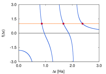
Figure 8: (color online) RPA secular equation for a paramagnetic system of $N=18$ particles at $r_{s}=1$, and $\bm{q}_{2}$. The blue solid line is the right member $f(\Delta\epsilon)$ of (63), and the orange dashed line is the constant function $g(\Delta\epsilon)=1$; intersections between the two graphs are marked with red dots. the RPA eigenvalues are the abscissae of such intersections.

We have seen that the RPA approximation yields an Ansatz for the energies $\epsilon_{\bm{q},n}$ and wavefunctions $|\Phi_{\bm{q},n}\rangle$ of excited states with definite momentum $\bm{q}$, which results in the following approximation for the image of the RPA ground state through the density fluctuation operator $\hat{\rho}_{\bm{q}}$:

$$\hat{\rho}_{\bm{q}}|\Phi_{0}\rangle=\sum_{n}|\Phi_{\bm{q},n}\rangle\langle\Phi_{\bm{q},n}|\hat{\rho}_{\bm{q}}|\Phi_{0}\rangle$$ (66)

with:

$$\langle\Phi_{\bm{q},n}|\hat{\rho}_{\bm{q}}|\Phi_{0}\rangle=\sum_{\begin{subarray}{c}|\bm{k}|\leq k_{F}\\ |\bm{k+q}|>k_{F}\end{subarray}}X_{\bm{k},n}+\sum_{\begin{subarray}{c}|\bm{k}|>k_{F}\\ |\bm{k+q}|\leq k_{F}\end{subarray}}Y_{\bm{k},n}$$ (67)

and for the dynamical structure factor:

$$S(\bm{q},\omega)=\frac{1}{N}\sum_{n}\delta(\omega-\epsilon_{\bm{q},n})|\langle\Phi_{\bm{q},n}|\hat{\rho}_{\bm{q}}|\Phi_{0}\rangle|^{2}$$ (68)

References

- (1) E. P. Wigner, Phys. Rev. 46, 1002 (1934)
- (2) F. Bloch Z. Phys. 57, 549 (1929)
- (3) A. W. Overhauser, Phys. Rev. Lett. 3, 414 (1959)
- (4) D. Ceperley, Phys. Rev. B 18, 3126 (1978); D. M. Ceperley and B. J. Alder, Phys. Rev. Lett. 45, 566 (1980)
- (5) G. F. Giuliani and G. Vignale, Quantum Theory of the Electon Liquid, Cambridge University Press (2005)
- (6) S. Zhang and D. Ceperley, Phys. Rev. Lett. 100, 236404 (2008)
- (7) For a comprehensive review of the existing quantum chemistry methodologies see for example the book: A. Szabo, and N.S. Ostlund, Modern Quantum Chemistry: Introduction to Advanced Electronic Structure Theory, Dover Publications (1996)
- (8) A. L. Fetter and J. D. Walecka, Quantum Theory of Many-Particle Systems, Dover (2003)
- (9) B. Tanatar and D. M. Ceperley, Phys. Rev. B 39, 5005 (1989)
- (10) Y. Kwon, D. M. Ceperley and R. M. Martin, Phys. Rev. B 48, 12037 (1993)
- (11) S. Moroni, D. M. Ceperley and G. Senatore Phys. Rev. Lett. 75, 689 (1995)
- (12) M. Padmanabhan, T. Gokmen, N. C. Bishop, and M. Shayegan, Phys. Rev. Lett. 101, 026402 (2008)
- (13) T. Gokmen, M. Padmanabhan, K. Vakili, E. Tutuc, and M. Shayegan, Phys. Rev. B 79, 195311 (2009)
- (14) Y.-W. Tan, J. Zhu, H. L. Stormer, L. N. Pfeiffer, K. W. Baldwin, and K. W. West, Phys. Rev. Lett. 94, 016405 (2005)
- (15) R. P. Feynman and A. R. Hibbs Quantum Mechanics and Path Integrals, McGraw-Hill (1965)
- (16) E. Y. Loh et al., Phys. Rev. B 41, 9301 (1990)
- (17) J. Anderson, J. Chem. Phys. 69, 1499 (1975)
- (18) P. J. Reynolds, D. M. Ceperley, B. J. Alder and W. A. Lester, J. Chem. Phys. 77, 5593 (1982)
- (19) M. Motta, D. E. Galli, S. Moroni and E. Vitali, J. Chem. Phys. 140, 024107 (2014)
- (20) D. M. Ceperley, J. Stat. Phys. 63, 1237 (1991)
- (21) G. H. Booth, A. J. W. Thom and A. Alavi J.Chem. Phys 131, 054106 (2009)
- (22) M. Feldbacher and F. F. Assaad Phys. Rev. B 63, 073105 (2001)
- (23) D. M. Ceperley and B. Bernu, J. Chem. Phys. 89, 6316 (1988); P.-M. Zimmerman, J. Toulouse, Z. Zhang, C.-B. Musgrave, C.-J. Umrigar J. Chem. Phys. 131, 124103 (2009)
- (24) M. Nava, A. Motta, D. E. Galli, E. Vitali and S. Moroni Phys. Rev. B 85, 184401 (2012)
- (25) G. H. Booth and G. Chan J. Chem. Phys. 137, 191102 (2012)
- (26) G. H. Booth, G. Chan Phys. Rev. B 91, 155107 (2015)
- (27) R. Blankenbecler, D. J. Scalapino and R. L. Sugar Phys. Rev. D 24, 2278 (1981)
- (28) G.Sugiyama and S. E. Koonin Ann. Phys. 168, 1 (1986)
- (29) S. Zhang and H. Krakauer, Phys. Rev. Lett. 90, 136401 (2003)
- (30) S. Zhang, H. Krakauer, W. A. Al Saidi and M. Suewettana Comp. Phys. Comm. 169, 394 (2005)
- (31) S. Zhang in Theoretical Methods for Strongly Correlated Electron Systems Springer Verlag (2003)
- (32) S. Zhang, J. Carlson and J. E. Gubernatis Phys. Rev. B 55, 7464 (1997)
- (33) W. Purwanto and S. Zhang, Phys. Rev. E 70, 056702 (2004)
- (34) W. Purwanto, S. Zhang and H. Krakauer J. Chem. Phys. 130, 094107 (2009)
- (35) W. Purwanto, H. Krakauer, Y. Virgus and S. Zhang J. Chem. Phys. 135, 164105 (2011)
- (36) W. Purwanto, H. Krakauer and S. Zhang Phys. Rev. B 80, 214116 (2009)
- (37) K. Sawada, Phys. Rev. 106, 372 (1957)
- (38) S. Baroni and S. Moroni, Phys. Rev. Lett. 82, 4745 (1999)
- (39) J. Toulouse and C. J. Umrigar, J. Chem. Phys. 128, 174101 (2008)
- (40) M. Motta, G. Bertaina, D. E. Galli and E. Vitali, Comp. Phys. Comm. 190 62-71 (2015)
- (41) P. P. Ewald Ann. Phys. 369, 253 (1921)
- (42) W. M. C. Foulkes, L. Mitas, R. J. Needs and G. Rajagopal Rev. Mod. Phys. 73, 33 (2001)
- (43) H. F. Trotter Proc. Amer. Math. Soc. 10, 545 (1959)
- (44) M. Suzuki Progr. Theor. Phys. 56, 1454 (1976)
- (45) J. Hubbard, Phys. Rev. Lett. 3, 77 (1959)
- (46) R. L. Stratonovich, Sov. Phys. Doklady 2, 416 (1957)
- (47) A. M. Turing, Q. J. Mech. Appl. Math. 1, 287 (1948)
- (48) A. N. Tikhonov and V. Y. Arsenin, Solution of Ill-posed Problems, Winston & Sons (1977)
- (49) R. Balian, E. Brezin, Il Nuovo Cimento B 64, 37 (1969)
- (50) T. Gaskell, Proc. Phys. Soc. 77, 1182 (1961); T. Gaskell, Proc. Phys. Soc. 80, 1091 (1962)
- (51) E. Vitali, M. Rossi, L. Reatto and D. E. Galli Phys. Rev. B 82, 174510 (2010)
- (52) K. Levenberg Quart. Appl. Math. 2 164 (1944); D. Marquardt SIAM J. Appl. Math. 11 431 (1963)
- (53) J. J. Shepherd, G. H. Booth, A. Grüneis, and A. Alavi, Phys. Rev. B 85, 081103(R) (2012)
- (54) J. J. Shepherd, G. H. Booth and A. Alavi J. Chem. Phys. 136, 244101 (2012)
- (55) H. Shi, S. Zhang Phys. Rev. B 88, 125132 (2013)
- (56) F. Ma, W. Purwanto, S. Zhang, H. Krakauer Phys. Rev. Lett. 114, 226401 (2015)
- (57) E. Y. Loh Jr., J. E. Gubernatis, R. T. Scalettar, R. L. Sugar and S. R. White, Interacting Electrons in Reduced Dimensions, NATO ASI Series 213 55-60 (1989)
- (58) C. N. Gilbreth and Y. Alhassid, Comp. Phys. Comm. 188 1-6 (2014).
- (59) L. Fox, H. D. Huskey and J. H. Wilkinson, Q. J. Mech. Appl. Math. 1, 149 (1948)
- (60) I. Tamm, J. Phys. (USSR) 9, 499 (1945)
- (61) S. M. Dancoff, Phys. Rev 78, 382 (1950)