Wealth distribution across communities
of adaptive financial agents

Abstract

This paper studies the trading volumes and wealth distribution of a novel agent-based model of an artificial financial market. In this model, heterogeneous agents, behaving according to the Von Neumann and Morgenstern utility theory, may mutually interact. A Tobin-like tax (TT) on successful investments and a flat tax are compared to assess the effects on the agents’ wealth distribution. We carry out extensive numerical simulations in two alternative scenarios: i) a reference scenario, where the agents keep their utility function fixed, and ii) a focal scenario, where the agents are adaptive and self-organize in communities, emulating their neighbours by updating their own utility function. Specifically, the interactions among the agents are modelled through a directed scale-free network to account for the presence of community leaders, and the herding-like effect is tested against the reference scenario. We observe that our model is capable of replicating the benefits and drawbacks of the two taxation systems and that the interactions among the agents strongly affect the wealth distribution across the communities. Remarkably, the communities benefit from the presence of leaders with successful trading strategies, and are more likely to increase their average wealth. Moreover, this emulation mechanism mitigates the decrease in trading volumes, which is a typical drawback of TTs.

1 Introduction

Neoclassical economics plays a fundamental role in the study of price and income distributions in markets [1]. Recent studies are focused on the development of tools and approaches that may complement neoclassical economics, removing some of its main assumptions, such as rationality and homogeneity of the financial agents [2, 3]. A special interest emerged for a complex system approach, which involves the use of agent-based and behavioural models [4, 5, 6, 7, 3, 8, 9, 10, 11, 2, 12, 13, 14, 15, 16, 17, 18, 19, 20]. In this way, the simulated behaviour of a high number of decision-makers and institutions (the agents), interacting through prescribed rules, can be investigated to highlight the macro features of the market emerging from the dynamic interactions among the players.

In the last decades, notable artificial financial models have been developed. The model in [11] provides a tenable explanation for bubbles and crashes, replicating liquidity crashes that cannot be predicted with equilibrium models. The studies in [21, 22] support the idea that scaling and fluctuations in financial prices arise from mutual agents’ interactions rather than from the efficient market hypothesis. The dynamics of companies’ growth and decline have been reproduced in [23], reflecting the power-law distribution of company size. In agent-based financial markets, agents can be modelled as zero-intelligence traders, acting randomly with a budget constraint [24], or as heterogeneous agents with bounded rationality, endowed with utility functions, who can envision strategies with limited complexity [10, 25, 7]. Moreover, agents may have the capability of adapting their actions according to their current state, the information gathered from the environment [26], and the rules governing their behaviour [27]. Different types of adaptive behaviour may be considered, such as learning, search and imitation [28]. Indeed, the capability of an investor of imitating the actions of others is one of the key elements of the widespread phenomenon of herding in financial markets [29, 30, 31, 32]. The concepts of learning and adaptation are also applied to utility functions, that may not be fixed, as observed in [33, 34, 32].

Agent-based approaches have also been used to test the effects of policies, regulations and taxation systems on the market dynamics, see for instance [15, 16]. Inspired by the seminal work of Tobin [35], several taxes on financial transactions were proposed to regulate the markets, whose effects have been controversial [36, 37]. The effect of taxation was also investigated in the kinetic exchange market models, see [17, 18, 19, 20] and references therein. In [17, 18], the authors reviewed the recent advances in the study of income and wealth distribution. In particular, they focused on the kinetic exchange market models and illustrated their microeconomic foundations. In [19], an ad hoc stochastic asset evolution was considered which explained the gamma-function-like income distribution. Later, Ref. [20] provided a microeconomic framework to derive asset equations consistent to those used in the ideal gas market models: at each time step, the agents randomly meet to transact according to the maximization of their Cobb-Douglas utility function. The authors analysed the steady-state income distribution for different values of a redistribution parameter, which mitigates the inequalities in wealth distribution. In particular, in [20] the steady-state wealth distribution was observed to be gamma-function-like, and studied in presence of a redistributive tax.

To the best of our knowledge, none of the existing models of artificial markets accounts for herding phenomena and different taxation schemes at the same time. In this work, we build a novel artificial financial market capable of testing the delicate interplay between herding-like interactions, the inequality in wealth distribution, and the balancing of two common alternative taxation schemes. The agents behave according to utility theory, and are grouped in three classes with different risk attitudes and subsequent trading strategies. We study the emerging features of the market in terms of trading volumes and wealth distribution, characterized through the Gini coefficient [38], in presence of a Tobin-like tax (TT) and a flat tax (FT), respectively. Specifically, we investigate two agents’ behavioural scenarios: i) stubborn agents [39], who keep their own risk attitude regardless of the effectiveness of the consequent trading strategy (reference scenario); ii) adaptive agents, who self-organize in communities to emulate the strategy of their richest neighbours (focal scenario). These latter act as leaders and are modelled as the hubs of a directed scale-free network [40].

The outline of the paper is as follows. In section 2, we describe the proposed model of a financial market in terms of agents behaviour, alternative taxation schemes, and interaction rules. In section 3, the focal scenario is tested against the reference one. The interplay between the different taxation systems and agents’ behavioural adaptation is analysed, with a special emphasis on the effects on wealth distribution and trading volumes. Finally, conclusions are drawn in section 4.

2 The model

We introduce an agent-based model of a financial market populated by a set of $n$ agents, who can choose among alternative financial assets. The state of each agent $j$ is defined as his current wealth $x_{j}$ and risk attitude $\alpha_{j}$. The agents behave according to the Von Neumann and Morgenstern utility theory [41], and alternative taxation schemes and interaction rules are considered.

2.1 Market structure

At time $0$, the state of agent $j$ is given by his initial wealth and risk attitude, denoted $x_{j0}$ and $\alpha_{j0}$, respectively, $j=1,\ldots,n$. At each time step $k=1,2,...$, a simulated trading session is performed. Each agent, in a sequential random order, evaluates the convenience of investing a given fraction $\delta$ of his current wealth $x_{j}(k)$ in one of the financial assets from the set $\mathcal{I}=\{1,\ldots,m\}$. The assets in $\mathcal{I}$ are characterized by a limited availability $A_{i},i=1,...,m$, where $A_{m}=+\infty$ is associated to a virtual asset, corresponding to no-investment. In view of this, each agent is allowed to invest in one of the available assets, that is, in any element of $\mathcal{I}$ such that $A_{i}\geq\delta x_{j}(k)$. Agents’ access to trading is randomly permuted at each time step $k$, so that, on average, no agent is favoured. After each trading, the availability of the selected asset is updated before the next agent is allowed to trade.

2.2 Agent behaviours

2.2.1 Agent trading strategy

A power-law utility function characterizes the risk attitude of each agent. At each trading session $k$, agent $j$ decides to invest a fraction $\delta$ of its current wealth $x_{j}(k)$ in the most profitable asset $i\in\mathcal{I}$, selected by comparing the expected utilities

$$E[U_{j}(x_{j}(k),i)]=0.5\left[(a_{i}\delta x_{j}(k))^{\alpha_{j}(k)}+(b_{i}\delta x_{j}(k))^{\alpha_{j}(k)}\right],\ i=1,...,m,$$ (1)

where ${{\alpha}_{j}}(k)$ is a (possibly time-varying) coefficient which determines the risk attitude of the j-th agent, $a_{i}$ and $b_{i}$ are the win and loss rates associated to the i-th asset, $i=1,\ldots,m$ . Based on their current risk attitude, we group the agents in three classes. In the first one, there are the agents characterized by a low risk attitude, denoted in what follows as prudent agents. The agents that are more prone to take risks are denoted audacious and grouped in the third class. Finally, the intermediate class groups the ordinary agents. We emphasize here that an agent may decide not to invest (formally, to invest in the $m$-th asset), if $E[U_{j}(x_{j}(k),m)]\geq E[U_{j}(x_{j}(k),i)]$ for all $i=1,\ldots,m-1$. The outcome of the trade is the realization $\beta$ of a uniform Bernoulli random variable $B$. Therefore, the wealth $x_{j}^{-}(k)$ of the agent $j$ at time $k$ before the taxation is given by:

$$x^{-}_{j}(k)=x_{j}(k-1)+\beta\delta x_{j}(k)(a_{i}-1)-(1-\beta)\delta x_{j}(k)(1-b_{i}).$$ (2)

When the trading session is over, a tax is applied and the wealth of agent $j$ at time $k$ is updated as

$$x_{j}(k)=\tau(x^{-}_{j}(k)),$$ (3)

where $\tau$ is the function describing the selected taxation scheme, see section 2.4.

2.2.2 Interaction among the agents

We consider two alternative scenarios. In the reference scenario, the market is composed of stubborn agents, who do not modify their utility function even if they observe that their investing strategy is not successful. Accordingly, their risk attitude is considered as a parameter rather than an evolving state, that is, $\alpha_{j}(k)=\alpha_{j0}$, for all $k\in\mathbb{N}$, $j=1,\ldots,n$. In the focal scenario, instead, the agents are adaptive, as they are prone to directly interact with each other and update their trading strategy. In particular, we model the strategy modification as a variation of the coefficient $\alpha_{j}(k)$ in (1). We emphasize that $\alpha_{j}(k)$ is referred to as “risk attitude” for simplicity, but it may also embed other relevant factors determining the expected utility function of agent $j$, such as the perceived information level of the other investors [32]. The reciprocal influence among the agents diffuses through a connection topology described by a directed graph $\mathcal{G}=\{{\mathcal{V},\mathcal{E}}\}$, where $\mathcal{V}$ is the set of nodes, corresponding to the agents, and $\mathcal{E}$ is the set of directed edges connecting the nodes. The existence of an edge $(i,j)$ implies that the risk attitude of node $j$ is influenced by that of node $i$. The herding-like dynamics of the coefficients $\alpha_{j}(k)$ in (1) is described by

$$\alpha_{j}(k)=(1-w)\alpha_{j}(0)+\frac{w}{|\mathcal{N}_{j}|}\sum_{h\in\mathcal{N}_{j}}\alpha_{h}(k-1),$$ (4)

where $w$ is the interaction weight, $\alpha_{j}(0)=\alpha_{j0}$, and $\mathcal{N}_{j}$ is the set of the neighbours of the j-th agent, defined as $\mathcal{N}_{j}=\left\{i\in\mathcal{V}:(i,j)\in\mathcal{E}\right\}$. We remark that the bigger the coefficient $w$ is, the more the agents are prone to modify their utility function: $w=0$ models the case of stubborn agents, while $w=1$ the case in which the agents completely disregard their innate risk attitudes and emulate the neighbours’ behaviour.

2.3 Leaders and communities

The interaction topology is modelled as a disjoint directed scale-free network, and the graph $\mathcal{G}$ is decomposed in up to three disconnected components, the communities, each of which is guided by leaders belonging to the same risk attitude class. Namely, inside each community, we consider emulating the rich dynamics, where the richest agents are stubborn, but influence the other agents, so playing the role of leaders [42]. We choose to consider separated communities so that each follower cannot be influenced by leaders with significantly different risk attitudes. Accordingly, each follower elects to emulate the strategy he considers most profitable. The size of the communities is proportional to the total wealth of their leaders and, inside each community, the richest agents are more likely to activate links.

The interaction is triggered at a given time instant $k_{t}$. Henceforth, the dynamics of $\alpha_{j}(k)$, $j=1,...,n$, described in (4), are strongly influenced by the structure of the graph $\mathcal{G}$ describing the diffusion flow. In turn, the structure of $\mathcal{G}$ is established at time $k_{t}$, based on the current wealth $x_{j}(k_{t})$, for $j=1,\ldots,n$.

2.4 Taxation schemes

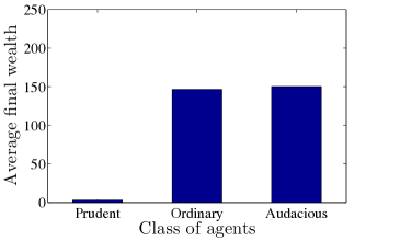
Figure 1: Reference scenario. Final wealth distribution when TT 1 and FT 1 schemes are introduced, respectively.

We consider two alternative taxation systems, which affect the current wealth of the agents $x^{-}_{j}(k)$ in different ways: a) taxation on financial transactions, and b) taxation on wealth. Type a) tax is a Tobin-like tax, which reduces the current wealth of the winning agents by a profit fraction $u(k)$ given by

$$u(k)=\left\{\begin{array}[]{ll}\frac{p(k)}{\sum_{j=1}^{n}s_{j}(k)},\ \ \,p(k)>0,\\ 0,\qquad\qquad p(k)\leq 0,\end{array}\right.$$ (5)

where $s_{j}(k)=x^{-}_{j}(k)-x_{j}(k-1)$, and $p(k)=\sum_{j=1}^{n}(x^{-}_{j}(k)-x_{j0})$. Accordingly, (3) becomes

$$x_{j}(k)=x^{-}_{j}(k)-H(s_{j}(k))s_{j}(k)u(k),$$ (6)

where $H$ is the Heaviside step function.

The alternative taxation scheme b) is a FT, in which the amount of the tax is proportional to the total wealth of the individual. Accordingly, (3) becomes

$$x_{j}(k)=v(k)x^{-}_{j}(k),$$ (7)

where $v(k)=\frac{\sum_{j=1}^{n}x_{j0}}{\sum_{j=1}^{n}x^{-}_{j}(k)}$.

Notice that, to allow for a proper comparison between the two taxation schemes, the coefficients $u(k)$ and $v(k)$ in (5) and (7), respectively, are selected so as to keep the average wealth constant over time, that is, $\frac{1}{n}\sum_{j=1}^{n}x_{j}(k)=\bar{x}$.

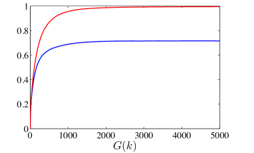
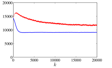
Figure 2: Reference scenario. Gini coefficient 2 and trading volumes 2 when TT (blue line) and FT (red line) schemes are introduced, respectively.

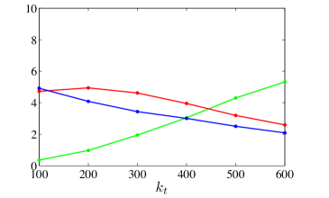
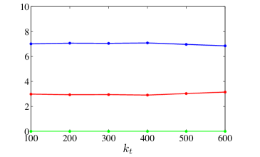
Figure 3: Focal scenario. Average number of leaders of belonging to the communities 1 (red line), 2 (blue line) and 3 (green line) for different interaction triggering time $k_{t}$ when TT 3 and FT 3 schemes are introduced, respectively.

Figure 4: Final wealth distribution when TT scheme is introduced: reference 4 and focal 4 scenarios, respectively. The width of the bars is proportional to the numerosity of the classes.

3 Results

The proposed model of artificial financial market can take into account different scenarios, in terms of both taxation schemes and interaction rules. In this section, we analyse the emerging features in the focal scenario, aiming at identifying the possible interplay between taxation and interaction in determining the trading volumes and the wealth distribution among the agents. To do so, we compare the results of extensive simulations of the focal scenario against those of the reference one. The effect of the alternative taxation schemes are firstly pointed out in the reference scenario. Then, we focus on adaptive agents and study the effects induced by the emulating dynamics on the wealth distribution for both taxation schemes. To achieve statistical relevance, we run 1000 simulations for each scenario and consider a number of time steps sufficient to reach steady-state wealth distribution.

We consider $n=1000$ agents that share the same initial capital $x_{j0}=100\$$, $j=1,\ldots,n$, and, at each trading session $k$, can decide to invest a fraction $\delta=0.2$ of their current wealth. The cardinality of the set of assets $\mathcal{I}$ is $m=4$, that is, the agents can trade in three categories of actual assets, while the fourth one corresponds to no-investment and, therefore, has an unlimited availability. On the other hand, at every time instant, each of the three actual assets has an availability equal to $1/15$th of the total wealth of the system. The win and loss rates associated to the actual assets are selected so that the prudent agents $(0.5\leq\alpha_{j}(k)<0.67)$ only consider investing in the first and less risky asset, the ordinary agents $(0.67\leq\alpha_{j}(k)<0.83)$ also consider the second, while the audacious agents $(0.83\leq\alpha_{j}(k)\leq 1)$ also find convenient investing in the third and most risky one. Namely, the won rates are $a_{1}=1.53$, $a_{2}=1.60$, and $a_{3}=1.67$, while the loss rates are $b_{1}=0.6$, $b_{2}=0.5$, and $b_{3}=0.4$. Notice that, with this parameter selection, $E[U_{j}(x_{j}(k),1)]>E[U_{j}(x_{j}(k),2)]>E[U_{j}(x_{j}(k),3)]$, $j=1,...,n$. The initial risk attitudes $\alpha_{j0}$, $j=1,...,n$, are uniformly distributed in the interval $[0.5,1]$.

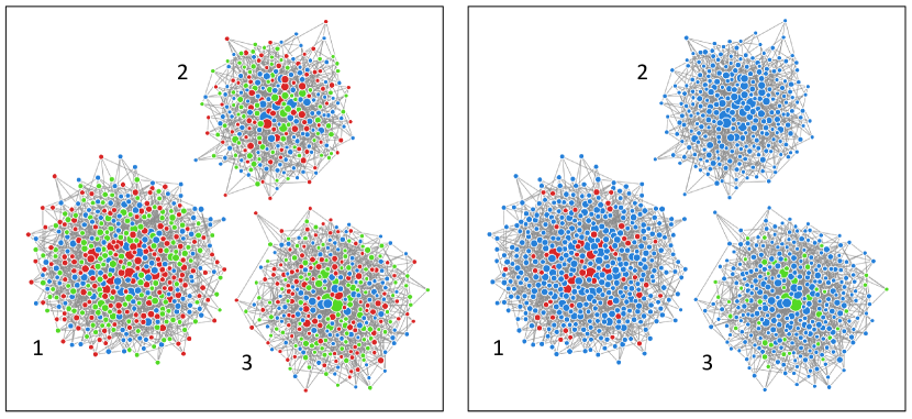
Figure 5: Focal scenario, TT scheme. Screenshots of the three communities before (left panel) and after (right panel) the herding-like effect in a sample simulation. The red, blue, and green nodes correspond to prudent, ordinary, and audacious agents, respectively. Notice that the averaging of the attitudes increases the overall density of ordinary agents. However, the leaders’ influence skews the distribution across the communities, with prudent and audacious agents still populating the first and third community, respectively.

3.1 Reference scenario

In our numerical analysis, we monitor the effect of the alternative taxation schemes on both the wealth distribution and the trading volumes in the artificial market. Specifically, we observe that the TT scheme hinders the audacious agents, favouring the prudent ones. This is clearly depicted in figure 11, which shows the sum of the average final wealth in the three classes of agents, respectively. The opposite is observed when a flat tax is adopted, in which the wealth distribution is biased towards the ordinary and audacious agents, see figure 11. In other words, the TT scheme does not reward the risk, penalizing the audacious agents, in opposition to the FT scheme, which encourages the agents to trade.

A second striking difference among the two taxation schemes is the overall wealth dispersion. To point out this emerging feature, we consider the Gini coefficient $G(k)$, proposed by Corrado Gini in [38] as a measure of inequality of income or wealth, which can be defined as

$$G(k)=1-\frac{2}{n-1}\left(n-\frac{\sum_{j=1}^{n}jx_{j}(k)}{\sum_{j=1}^{n}x_{j}(k)}\right),$$ (8)

where the wealths $x_{j}(k)$, $j=1,\ldots,n$, are indexed in non-decreasing order $(x_{j}(k)\leq x_{j+1}(k))$. The Gini coefficient varies between 0, which reflects complete equality, and 1, which indicates complete inequality (one person holds the all wealth, all others have none). As depicted in figure 22, while the TT scheme induces a wealth redistribution among the population, the FT scheme increases inequalities. On the other hand, the TT scheme leads to lower trading volumes at the steady-state, see figure 22. The latter effect is in line with the criticisms commonly made to financial transaction taxes, which are blamed for possible market depression [43, 36, 44].

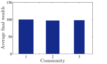
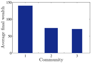
Figure 6: Average final wealth of the agents belonging to communities 1, 2 and 3, when TT scheme is introduced: reference 6 and focal 6 scenarios, respectively.

3.2 Focal scenario

We assume that, after $k_{t}$ time steps in which the agents invest based on their own risk attitude, the emulation dynamics described in (4) are triggered. The triggering instant of the emulation behaviour is indifferent to our purpose, as alternative values of $k_{t}$ only affect the size of the communities, see figure 3. The ten richest agents (the leaders) are assumed to have only outgoing edges; the followers, instead, have bidirectional edges with their neighbouring peers, and may have ingoing edges from the leaders. To model this interaction mechanism, we build a directed Barabási-Albert (BA) scale-free network [40], in which the hubs coincide with the leaders. The network is split into three communities, led by the prudent, ordinary, and audacious leaders, respectively. The size of each community is proportional to the sum of the leaders’ wealth, which is an indirect measure of their influence.

The results are compared against a twin set of simulations in the reference scenario, sharing the same set of realizations of the Bernoulli variable $B$ in (2). For the sake of clarity, we analyse the two taxation schemes separately, starting with the TT scheme. From figure 4, we observe that this taxation system, regardless of the interactions among the agents, recompenses the prudent strategies in the long run. The emulating the rich interaction, instead, skews the distribution among the communities, see figure 5. In absence of leaders, the interaction with the neighbours would tend to average the agents’ attitudes towards risk. However, the presence of leaders differentiates the communities. In particular, the community guided by the prudent leaders preserves a significant number of prudent agents (the 20.29% of the total population of the community, see table 1). Consequently, the average wealth of the agents in the first community is considerably higher compared with the other two communities (see figure 66), whose leaders pursue risky strategies which turn to be unprofitable in the long term (their steady-state capital is lower than the average agents’ wealth $\bar{x}=100$, see table 2).

Moreover, figure 7 shows that the herding mechanism has the further effect of mitigating the decrease in trading volumes typical of the TT case. This is due to the reduction of the total number of prudent agents illustrated in figure 4. Differently from the TT case, in which the prudent agents slowly but relentlessly take the leadership of the market, see figure 33, when the flat tax is introduced, a prudent strategy is disadvantageous both in the short and in the long term, see figure 33. Consequently, no agent is encouraged to emulate the prudent agents, and the market splits into only two communities, guided by the ordinary and audacious leaders, respectively. Accordingly, there are no notable differences in the average wealth of the two communities, see table 1. We emphasize that, while the emulating dynamics can strongly influence the distribution of the wealth across the communities, the overall wealth distribution is only dictated by the taxation scheme. In particular, the variation of the Gini coefficient induced by the emulation dynamics is an order of magnitude lower than that induced by a change of taxation scheme, for any possible value of the interaction weight $w$ and of the average degree of the connection topology.

Table 1: Legend. $\bar{x}_{r}(T)$ and $\bar{x}_{f}(T)$ are the average final wealth in the reference and focal scenarios, respectively; $\nu_{c_{i}}$ is the average numerosity of the $i$-th community, $i=1,2,3$; $f_{j}$ is the final percentage of agents belonging to the $j$-th class, $j=1,2,3$. Confidence intervals with significance level $0.05$ are also reported.

•	Tobin Tax			Flat Tax
Community	1	2	3	1	2	3
$\bm{\bar{x}_{r}(T)/\bar{x}}$	1.01	0.97	0.98	0	1.07	0.97
	[0.99, 1.02]	[0.96, 0.99]	[0.97, 1.00]		[1.01, 1.13]	[0.94, 1.01]
$\bm{\bar{x}_{f}(T)/\bar{x}}$	1.40	0.74	0.71	0	1.05	0.98
	[1.38, 1.42]	[0.73, 0.75]	[0.70, 0.73]		[0.99, 1.11]	[0.95, 1.01]
$\bm{\nu_{c_{i}}}$	380.76	347.63	271.61	$\ \ 0\$	246.24	753.76
	[369.89, 391.01]	[336.54, 357.92]	[260.91, 281.71]		[235.76, 256.19]	[742.78, 763.20]
$\bm{f_{1}}$(%)	20.29	0.60	0.01	0	0.80	0
	[19.78, 20.80]	[0.53, 0.66]	[0.01, 0.02]		[0.69, 0.92]
$\bm{f_{2}}$(%)	79.71	99.40	93.04	0	99.16	93.13
	[79.20, 80.21]	[99.32, 99.45]	[92.67, 93.41]		[99.04, 99.27]	[92.95, 93.32]
$\bm{f_{3}}$(%)	0	0	6.95	0	0.04	6.87
			[6.58, 7.32]		[0.03, 0.06]	[6.68, 7.05]

We remark that considering disconnected communities is an idealization of real-world aggregations, where few weak links may still connect the communities. However, all the presented results are robust to the addition of links connecting the communities. This is confirmed by a twin set of simulations in which a small fraction (less than 5%) of the network edges are rewired following a degree-preserving procedure inspired by the work in [45]. Considering 95% confidence intervals, we find that the variations of the results are not statistically significant.

Table 2: Legend. $\bar{x}_{l}(T)$ is the average final wealth of the leaders in the focal scenario; $\nu_{l_{i}}$ is the average numerosity of the leaders of the $i$-th community, $i=1,2,3$. Confidence intervals with significance level $0.05$ are also reported.

	Leaders	L1	L2	L3
	$\bm{\bar{x}_{l}(T)/\bar{x}}$	7.69	0.66	0.64
Tobin Tax		[7.18,8.19]	[0.59,0.72]	[0.37,0.90]
	$\bm{\nu_{l_{i}}}$	4.30	3.20	2.50
		[4.20,4.40]	[3.10,3.29]	[2.41,2.59]
	$\bm{\bar{x}_{l}(T)/\bar{x}}$	0	14.29	14.48
Flat Tax			[12.60,15.98]	[13.24,15.71]
	$\bm{\nu_{l_{i}}}$	0	3.03	6.97
			[2.94,3.12]	[6.88, 7.06]

4 Discussion

In this paper, we presented a novel agent-based model of a financial market. The agent behaviour has been modelled according to the Von Neumann and Morgenstern utility theory, which led to the definition of three possible trading strategies. Based on the selected strategy, the agents were classified as prudent, ordinary, or audacious. The proposed model allowed for a numerical study of the interplay between herding-like dynamics, the wealth inequalities, and the redistributive effect of two common alternative taxation schemes. Specifically, we considered agents capable of adapting their utility function emulating the strategic behaviour of the successful agents. The emerging wealth distribution and trading volumes were compared against the reference scenario of stubborn agents, who maintain their beliefs regardless of the outcome of their trades. The analysis was carried out for two alternative taxation schemes, introducing a Tobin-like tax and a flat tax. The emerging features of the market have been investigated through a set of extensive simulations in a market populated by 1000 agents.

The numerical analysis of the reference scenario replicated the well known benefits and drawbacks of the two taxation schemes. Indeed, we observed a trade-off between wealth redistribution and trading volumes: while the Tobin-like tax has the effect of redistributing the wealth among the agents, but reduces the trading volumes, the opposite happens with a flat tax, which encourages to invest, but dramatically increases the disparity among the agents. Moreover, while the TT scheme favoured the prudent agents investing only in the less risky assets, the FT scheme rewarded the audacious agents, that also consider investing in the riskiest assets. In the focal scenario, where the adaptive agents consider adjusting their risk attitude and the consequent trading strategy, we observed a significant impact of the agents interactions on the emerging features of the market. Indeed, the richest agents, recognized as the market leaders, formed separate communities. Notably, we observed that the communities benefit from the presence of leaders with successful trading strategies, and are more likely to increase their average wealth. Moreover, this herding-like behaviour mitigated the reduction of the trading volumes typical of Tobin-like taxes, while preserving its redistributive effect. Ongoing works are devoted to further investigate the driving factors of herding, explicitly accounting for the effect of external inputs, such as the information gathered from the environment.

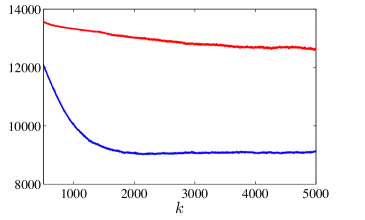
Figure 7: Trading volumes when TT scheme is introduced: reference (blue line) and focal (red line) scenarios, respectively.

References

- [1] Backhouse R 1985 A history of modern economic analysis (Oxford: Basil Blackwell)
- [2] Mantegna R N and Kertész J 2011 New Journal of Physics 13 025011
- [3] Cristelli M, Pietronero L and Zaccaria A 2010 Critical overview of agent-based models for economics Proceedings of the School of Physics ”E. Fermi”
- [4] Alfi V, Cristelli M, Pietronero L and Zaccaria A 2009 The European Physical Journal B-Condensed Matter and Complex Systems 67 385–397
- [5] Cavagna A, Garrahan J P, Giardina I and Sherrington D 1999 Physical Review Letters 83 4429
- [6] Pastore S, Ponta L and Cincotti S 2010 New Journal of Physics 12 053035
- [7] Cincotti S, Focardi S M, Marchesi M and Raberto M 2003 Physica A 324 227–233
- [8] Farmer J D and Foley D 2009 Nature 460 685–686
- [9] Gilbert N 2008 Agent-based models 153 (Sage)
- [10] LeBaron B 2001 Quantitative Finance 1 254–261
- [11] LeBaron B 2002 Building the Santa Fe artificial stock market Brandeis University, working paper
- [12] Tumminello M, Lillo F, Piilo J and Mantegna R N 2012 New Journal of Physics 14 013041
- [13] Westerhoff F 2010 New Journal of Physics 12 075035
- [14] San Miguel M, Johnson J H, Kertesz J, Kaski K, Díaz-Guilera A, MacKay R S, Loreto V, Érdi P and Helbing D 2012 European Physical Journal-Special Topics 214 245
- [15] Westerhoff F H and Dieci R 2006 Journal of Economic Dynamics and Control 30 293–322
- [16] Dignum F, Dignum V and Jonker C M 2009 Towards agents for policy making Multi-Agent-Based Simulation IX (Springer-Verlag) pp 141–153
- [17] Chakrabarti B K, Chakraborti A, Chakravarty S R and Chatterjee A 2013 Econophysics of Income and Wealth Distributions (New York: Cambridge University Press)
- [18] Pareschi L and Toscani G 2014 Interacting Multiagent Systems (Oxford, United Kingdom: Oxford University Press)
- [19] Guala S D 2009 Interdisciplinary Description of Complex Systems 7 1–7
- [20] Chakrabarti A S and Chakrabarti B K 2009 Physica A 388 4151–4158
- [21] Lux T and Marchesi M 1999 Nature 397 498–500
- [22] Zawadowski A G, Karadi R and Kertesz J 2002 Physica A: Statistical Mechanics and its Applications 316 403–412
- [23] Axtell R L 2001 Science 293 1818–1820
- [24] Gode D K and Sunder S 1993 Journal of Political Economy 101 119–137
- [25] Amilon H 2008 Journal of Empirical Finance 15 342–362
- [26] Lillo F, Miccichè S, Tumminiello M, Pillo J and Mantegna R N 2015 Quantitative Finance 15 213–229
- [27] Baek Y, Lee S H and Jeong H 2010 Physical Review E 82 026109
- [28] Blume L and Easley D 1992 Journal of Economic theory 58 9–40
- [29] Shapira Y, Berman Y and Ben-Jacob E 2014 New Journal of Physics 16 053040
- [30] Cipriani M and Guarino A 2009 Journal of the European Economic Association 7 206–233
- [31] Lillo F, Moro E, Vaglica G and Mantegna R N 2008 New Journal of Physics 10 043019
- [32] Decamps J P and Lovo S 2002 Available at SSRN 301962
- [33] Cohen M D and Axelrod R 1984 The American Economic Review 74 30–42
- [34] Cyert R M and DeGroot M H 1979 Adaptive utility Expected Utility Hypotheses and the Allais Paradox (Springer) pp 223–241
- [35] Tobin J 1978 Eastern Economic Journal 4 pp. 153–159 ISSN 00945056
- [36] Hanke M, Huber J, Kirchler M and Sutter M 2010 Journal of Economic Behavior & Organization 74 58–71
- [37] Li H, Tang M, Shang W and Wang S 2013 Procedia Computer Science 18 1764–1773
- [38] Gini C 1912 Reprinted in Memorie di metodologica statistica (Ed. Pizetti E, Salvemini, T). Rome: Libreria Eredi Virgilio Veschi 1
- [39] Porfiri M, Bollt E M and Stilwell D 2007 The European Physical Journal B-Condensed Matter and Complex Systems 57 481–486
- [40] Barabási A L and Albert R 1999 Science 286 509–512
- [41] Von Neumann J and Morgenstern O 2007 Theory of Games and Economic Behavior (60th Anniversary Commemorative Edition) (Princeton University Press)
- [42] Ellero A, Fasano G and Sorato A 2013 Physical Review E 87 042806
- [43] Baltagi B H, Li D and Li Q 2006 Empirical Economics 31 393–408
- [44] Mannaro K, Marchesi M and Setzu A 2008 Journal of Economic Behavior & Organization 67 445–462
- [45] Lancichinetti A, Fortunato S and Radicchi F 2008 Physical Review E 78 046110