Abstract

Recently, there has been much interest in holographic computations of two-point non-equilibrium Green functions from AdS-Vaidya backgrounds. In the strongly coupled quantum field theory on the boundary, the dual interpretation of the background is an equilibration process called a holographic quench. The two dimensional AdS-Vaidya spacetime is a special case, dual to conformal quantum mechanics. We study how the quench is incorporated into a Hamiltonian $H+\theta(t)\Delta H$ and into correlation functions. With the help of recent work on correlation functions in conformal quantum mechanics, we first rederive the known two point functions, and then compute non-equilibrium 3- and 4-point functions. We also compute the 3-point function Witten diagram in the two-dimensional AdS-Vaidya background, and find agreement with the conformal quantum mechanics result.

1 Introduction and summary

Partially motivated by the AdS/CFT correspondence, there has been recent progress in understanding correlation functions in conformally invariant quantum mechanics (CQM), relevant for the AdS₂/CFT₁ case. In this case, the $SO(2,1)$-isometry of the bulk AdS₂ manifold manifests as a $SO(2,1)$ conformal invariance of a quantum mechanical theory on the boundary.

The benchmark model of conformal quantum mechanics, viewed as the $D=1$ limit of $SO(D+1,1)$ conformally invariant scalar field theories with a $g\phi^{2D/(D-2)}$ potential in $D$ spacetime dimensions, was studied by de Alfaro, Fubini and Furlan (dAFF) [1]. The action is invariant under $SO(2,1)$ i.e. $SL(2,\mathbb{R})$ transformations, with the generators satisfying, after quantization, the commutation relations

$$i[D,H]=H,\quad i[D,K]=-K,\quad i[K,H]=2D$$ (1.1)

of a $so(2,1)$ Lie algebra. There are many other quantum mechanical realizations of (1.1) besides the original dAFF model. For the AdS₂/CFT₁ correspondence, we expect the relevant model to have many ($N$) interacting degrees of freedom, with the bulk calculations corresponding to a large $N$, strong coupling limit. However, the full picture of the AdS₂/CFT₁ correspondence is not yet well understood, due to complications arising from the AdS₂ fragmentation and backreaction when the geometry is reached from string theory in a form AdS${}_{2}\times X$ where $X$ is a compact space [2]. Recently, these issues were studied in context of 1+1 dimensional models of dilaton gravity coupled to matter [3]. There one can also construct solutions for an ingoing null matter pulse into a vacuum, creating a black hole, so that the two-dimensional spacetime is described by the AdS-Vaidya metric.

The null collapse to a black hole, or the AdS-Vaidya spacetime has been much studied as an analytic holographic model of one type of a global quench in the QFT on the boundary (see [4] for an early idea, and e.g. [5, 6, 7, 8, 9] for early papers on AdS-Vaidya and holographic quench). In particular, the model enables one to study nonequilibrium Green functions for a strongly coupled QFT, as these can be computed from the bulk geometry. However, it is not very transparent how exactly the quench is realized on the boundary. Furthermore, especially in higher dimensions the Green functions do not usually have a simple analytic form. In this paper, we are interested in studying the holographic quench in 0+1 dimensions, and the structure of the Green functions. We work in a simplified setting, assuming that the bulk spacetime is described by the two-dimensional AdS-Vaidya metric. For the dual theory at the boundary, we rely on the recent work [10], where the authors studied how to construct correlation functions in conformal quantum mechanics. Using only the $so(2,1)$ algebra, without specifying the underlying theory, they constructed operators which satisfied some, but not all properties of conformal primaries, and a vacuum state which was not fully invariant under (1.1). However, despite these shortcomings when the vacuum and the operators are combined to correlation functions, the result satisfies expected transformation properties for a conformally invariant theory.

In addition to the general motivation of extending the study of quenches modeled by AdS-Vaidya spacetimes to the AdS₂/CFT₁ case, we have specific motivations and goals: 1) it is interesting to study to what extent non-equilibrium correlation functions can be computed working directly on the boundary theory; 2) we would like to understand in more detail what kind of a quench the AdS-Vaidya bulk spacetime corresponds to in the boundary; 3) 3-pt and 4-pt correlation functions have been studied at thermal equilibrium [11] and more recently in the context of semiclassical limits by bulk geodesic methods [12, 13, 14], but not yet in the context of global quenches. In this work we interpret the AdS₂-Vaidya spacetime to be realized in CQM as a sudden change of the Hamiltonian. We compute analytic results for thermal and non-equilibrium 2-pt, 3-pt and 4-pt functions in quenched conformal quantum mechanics, by using the results of [10], and the 2-pt and 3-pt functions also from a bulk AdS₂-Vaidya background calculation, finding agreement with the results from the CQM computation.

This paper is organized as follows: Section 2 reviews some key concepts of conformal quantum mechanics and various choices of time evolution; in Section 3 we introduce the AdS₂-Vaidya spacetime as a model of a quench, which we find to be realized in CQM as a sudden change of the Hamiltonian, and then compute non-equilibrium two-point and 3-point correlation functions both by the holographic method from the bulk spacetime and by a direct calculation in CQM. Section 4 extends the CQM calculation to the 4-point function, and ends with some brief comments.

2 Review

We first review some key features of $so(2,1)$ representation theory. The energy eigenvalues (of $H$) are continuous and the eigenstates are all non-normalizable. In addition, there is no state that would vanish under all three generators i.e. that would be invariant under all the symmetry transformations. Let us then consider another complete set of orthonormal states. Moving to a new basis of operators with the commutators

$$R = \frac{1}{2}\left(\frac{K}{a}+aH\right),$$

$$L_{\pm} = \frac{1}{2}\left(\frac{K}{a}-aH\right)\pm iD\ ,$$ (2.1)

where $a$ is a constant with the dimension of time, the commutation relations become

$$[R,L_{\pm}]=\pm L_{\pm},\quad[L_{-},L_{+}]=2R\ ,$$ (2.2)

so that they form the Cartan-Weyl basis of the $so(2,1)$ algebra. The generator $R$ is compact with a discrete set of eigenstates. The discrete lowest weight representation can then be constructed using $L_{\pm}$ as raising and lowering operators. Explicitly:

$$R|n\rangle = r_{n}|n\rangle,$$ (2.3)

$$r_{n} = r_{0}+n\ ,\,\,\,n\in\mathbb{N}$$ (2.4)

$$\langle n^{\prime}|n\rangle = \delta_{n^{\prime},n},$$ (2.5)

$$L_{\pm}|n\rangle = \sqrt{r_{n}(r_{n}\pm 1)-r_{0}(r_{0}-1)}|n\pm 1\rangle,\mbox{ and}$$ (2.6)

$$|n\rangle = \sqrt{\frac{\Gamma(2r_{0})}{n!\Gamma(2r_{0}+n)}}(L_{+})^{n}|0\rangle\ ,$$ (2.7)

where $r_{0}$ is a parameter, the lowest weight of the representation, also connected to the eigenvalue $r_{0}(r_{0}-1)$ of the Casimir invariant $\mathcal{C}=\frac{1}{2}(HK+KH)-D^{2}=R^{2}-L_{+}L_{-}$ of the algebra. In particular, the lowest eigenstate $|0\rangle\equiv|n=0\rangle$ plays the role of a vacuum, called the $R$-vacuum. For a generic $r_{0}$, the eigenvalue equation implies that the $R$-vacuum cannot be annihilated by all the $so(2,1)$ generators.

One can also construct a continuous basis of states, $|\tau\rangle$. Using the conventions in [1, 10], the operators take the form

$$H = -i\frac{d}{d\tau}$$ (2.8)

$$D = -i(\tau\frac{d}{d\tau}+r_{0})$$ (2.9)

$$K = -i(\tau^{2}\frac{d}{d\tau}+2r_{0}\tau).$$ (2.10)

Constructing the operator $R$ in this basis, one can relate the $|n\rangle$ and $|\tau\rangle$ bases with the help of a differential equation:

$$\langle\tau|R|n\rangle=r_{n}\langle\tau|n\rangle=\frac{i}{2}\left[\left(a+\frac{\tau^{2}}{a}\right)\frac{d}{d\tau}+2r_{0}\frac{\tau}{a}\right]\langle\tau|n\rangle$$

$$\Rightarrow\beta_{n}(\tau)\equiv\langle\tau|n\rangle=(-1)^{n}\left[\frac{\Gamma(2r_{0}+n)}{n!}\right]^{\frac{1}{2}}\left(\frac{a-i\tau}{a+i\tau}\right)^{r_{n}}\frac{1}{\left(1+\frac{\tau^{2}}{a^{2}}\right)^{r_{0}}}$$ (2.11)

The constants in the expression are determined by the condition that the raising and lowering operators operate in the same way in both bases.

The $|\tau\rangle$ basis is not orthonormal, but the overlap of two states has the form

$$\langle\tau_{1}|\tau_{2}\rangle=\sum\limits_{n=0}^{\infty}\beta_{n}(\tau_{1})\beta_{n}^{*}(\tau_{2})=\Gamma(2r_{0})\left(\frac{a}{i2(\tau_{1}-\tau_{2})}\right)^{2r_{0}}\ ,$$ (2.12)

the same as for primary operators of conformal weight $r_{0}$ in a conformal theory. In [10], the authors gave an explicit interpretation of (2.12) as a vacuum 2-point function, constructing an operator $O(\tau)$ which reproduces the $|\tau\rangle$ states operating on the R-vacuum, $|\tau\rangle=O(\tau)|0\rangle$. Explicitly,

$$O(\tau)=N(\tau)\exp(-\omega(\tau)L_{+})\ ,$$ (2.13)

with

$$N(\tau) = [\Gamma(2r_{0})]^{1/2}\left(\frac{\omega(\tau)+1}{2}\right)^{2r_{0}}\ ,$$

$$\omega(\tau) = \frac{a+i\tau}{a-i\tau}\ .$$ (2.14)

so that

$$\langle\tau_{2}|\tau_{1}\rangle=\langle 0|O^{\dagger}(\tau_{2})O(\tau_{1})|0\rangle\ .$$ (2.15)

There are some issues with this form. While it does produce the correct state $|\tau\rangle$, the action of $O^{\dagger}$ on the $R$-vacuum just returns the R-vacuum multiplied with the normalization factor $N(\tau)$. This would cause the time-translation invariance to be lost when considering $\langle 0|O(\tau_{1})O^{\dagger}(\tau_{2})|0\rangle$. One could consider an alternative definition for $O$ which would still produce the same $|\tau\rangle$ states. We could use

$$O(\tau)=N(\tau)\exp[-\omega(\tau)L_{+}]\exp[-\omega^{*}(\tau)L_{-}]$$

With this definition, $O(\tau)$ would produce the same $|\tau\rangle$ states but this time $O^{\dagger}(\tau)$ produces the state $|\tau\rangle^{*}$, i.e. a state with complex conjugated coefficients. This operator is almost Hermitian, apart from the complexity of $N(\tau)$. This alternative definition is not necessary for the calculations in this paper.

However, there is another alternative form, suggested in [15]. They suggested

$$O(\tau)=\frac{[\Gamma(2r_{0})]^{1/2}}{2^{2r_{0}}}e^{i\tau H}e^{aH}$$ (2.16)

as it correctly reproduces the $|\tau\rangle$ state when acting on $|n=0\rangle$. The leftmost exponential gives the time evolution from the $|\tau=0\rangle$ state which the rightmost exponential prepares from the R-vacuum.

2.1 Alternative time evolutions

So far we have chosen $H=-i\frac{d}{d\tau}$ as the time evolution generator. Alternative choices have been considered previously in [15, 16, 17] and this enables one to compute Green functions periodic in imaginary time, associated with a finite temperature background. We motivate the alternative time evolution generators by reviewing the isometry of two-dimensional anti-de Sitter spacetime AdS₂.

Three metrics are often used in the context of AdS₂: the Poincaré metric (the metric written in the Poincaré coordinate patch covering a part of the spacetime manifold), the global metric (using the global coordinates patch that covers the full AdS covering space manifold), and the black hole metric (using a coordinate patch, which after periodic identification in imaginary time defines an anti-de Sitter black hole) (see [18] and Figure 3 therein for an illustration of the patches). The metrics have the form

$${\rm Global:}\ \ \ ds^{2}=\frac{R^{2}}{\cos^{2}\theta}(-dT^{2}+d\theta^{2}),\,\,-\infty<T<\infty,\,\,-\frac{\pi}{2}<\theta<\frac{\pi}{2}$$ (2.17)

$${\rm Poincar\'{e}:}\ \ \ ds^{2}=\frac{R^{2}}{z^{2}}(-d\tau^{2}+dz^{2}),\,\,-\infty<\tau<\infty,\,\,0<z<\infty$$ (2.18)

$${\rm Black\ hole:}\ \ \ ds^{2}=\frac{R^{2}}{u^{2}}\left(-\left(1-\frac{u^{2}}{u_{H}^{2}}\right)dt^{2}+\frac{du^{2}}{\left(1-\frac{u^{2}}{u_{H}^{2}}\right)}\right),\,\,-\infty<t<\infty,\,\,0<u<u_{H}$$ (2.19)

and the coordinates are related by the transformations

$$\tau\pm z = 2a\,\tan\left[(T\pm\theta\pm\frac{\pi}{2})/2\right],$$ (2.20)

$$z = \frac{2u}{1+\cosh(v/u_{H})+(u/u_{H})\sinh(v/u_{H})},\quad\tau-z=2u_{H}\tanh\left(\frac{v}{2u_{H}}\right),$$ (2.21)

$$v(u,t) = t-u_{H}\,{\rm artanh}\left(\frac{u}{u_{H}}\right).$$ (2.22)

Here, we used different symbols for the variables of different choices of metrics for the sake of clarity.

The Killing vector fields that generate the $SO(2,1)$ isometry of AdS₂ are represented in Poincaré coordinates by

$$H=-i\partial_{\tau}$$

$$D=-i\left(\tau\partial_{\tau}+z\partial_{z}\right)$$

$$K=-i\left[\left(\tau^{2}+z^{2}\right)\partial_{\tau}+2\tau z\partial_{z}\right]$$ (2.23)

After transforming to global coordinates, the Killing vector that generates time translations in global time $T$ is the linear combination (see also [19])

$$H_{G}=aH+\frac{K}{4a}=-i\partial_{T}\ .$$ (2.24)

Likewise, after transforming to black hole coordinates, time translations in the time $t$ are generated by the combination

$$H_{BH}=H-K/(2u_{H})^{2}=-i\partial_{t}\ .$$ (2.25)

On the (conformal) boundary of the spacetime, the relation between the different time coordinates reduces to

$$\tau=2a\,\tan(T/2)=2u_{H}\tanh(t/2u_{H})$$ (2.26)

The linear combinations (2.24) and (2.25) are the alternative time-evolution generators considered in [15]. Moving to conformal quantum mechanics, the generators are represented as infinitesimal translation operators when acting on the time basis states, e.g. $H|\tau\rangle=-i\frac{d}{d\tau}|\tau\rangle$. For the generators $H_{G},H_{BH}$, one needs to define new time states $|T\rangle,|t\rangle$ [15]. Since $|\tau\rangle=O(\tau)|0\rangle$, and (in correlation functions) $O(\tau)$ transforms under coordinate transformation like a primary of weight $r_{0}$, one defines new time states $|\tilde{t}\rangle$ by

$$|\tilde{t}\rangle=\left(\frac{dt}{d\tilde{t}}\right)^{r_{0}}|t=t(\tilde{t})\rangle\ ,$$ (2.27)

or in our case explicitly:

$$|T\rangle=a^{r_{0}}(\cos(T/2))^{-2r_{0}}|\tau=2a\tan(T/2)\rangle$$ (2.28)

$$|t\rangle=(\cosh(t/(2u_{H})))^{-2r_{0}}|\tau=2u_{H}\tanh(t/(2u_{H}))\rangle\ .$$ (2.29)

The different choices of a Hamiltonian are then represented in the different time state basis as

$$H_{P}|\tau\rangle=-i\frac{d}{d\tau}|\tau\rangle$$ (2.30)

$$H_{G}|T\rangle=-i\frac{d}{dT}|T\rangle$$ (2.31)

$$H_{BH}|t\rangle=-i\frac{d}{dt}|t\rangle\ ,$$ (2.32)

inherited from the time evolutions in the three customary AdS₂ coordinate patches. The two-point function $G_{2}(\tau_{2},\tau_{1})=\langle\tau_{2}|\tau_{1}\rangle$ can then be related to two-point functions $\langle T_{2}|T_{1}\rangle$ and $\langle t_{2}|t_{1}\rangle$ in terms of a simple rule. Although the operator $O(\tau)$ is not a primary one, it transforms as one in correlation functions evaluated with respect to the $R$-vacuum state $|0\rangle\equiv|n=0\rangle$,

$$\langle\tilde{t}_{2}|\tilde{t}_{1}\rangle\equiv\langle 0|\tilde{O}^{\dagger}(\tilde{t}_{2})\tilde{O}(\tilde{t}_{1})|0\rangle=\langle 0|\left(\frac{dt_{2}}{d\tilde{t}_{2}}\right)^{r_{0}}O^{\dagger}(t_{2}(\tilde{t_{2}}))\left(\frac{dt_{1}}{d\tilde{t}_{1}}\right)^{r_{0}}O(t_{1}(\tilde{t_{1}}))|0\rangle\ .$$ (2.33)

This leads to

$$\langle T_{2}|T_{1}\rangle=\langle 0|O^{\dagger}_{G}(T_{2})O_{G}(T_{1})|0\rangle=\frac{\Gamma(2r_{0})a^{2r_{0}}}{[4i\sin(\frac{T_{2}-T_{1}}{2})]^{2r_{0}}}$$

$$\langle t_{2}|t_{1}\rangle=\langle 0|O^{\dagger}_{BH}(t_{2})O_{BH}(t_{1})|0\rangle=\frac{\Gamma(2r_{0})a^{2r_{0}}}{[4u_{H}i\sinh(\frac{t_{2}-t_{1}}{2u_{H}})]^{2r_{0}}}\ .$$ (2.34)

3 AdS-Vaidya geometry and holographic quench

We now move to consider a holographic model of a quench, and incorporate it into conformal quantum mechanics. In gauge-gravity duality, a quench in the strongly coupled theory on the boundary has a holographic dual interpretation in the bulk AdS geometry. Perhaps the simplest and most popular model that has been studied is the AdS-Vaidya spacetime. It describes lightlike collapse of matter into a black hole in AdS_D+1 space. The holographic dual interpretation is that the theory on the $D$ spacetime dimensional boundary is initially in a vacuum state, then is at $t=0$ instantaneously sourced in a homogeneous manner into an excited state which then time evolves into thermal equilibrium. The initial non-equilibrium state is somewhat special, because expectation values of all local operators thermalize instantaneously. The non-equilibrium nature is only revealed by considering expectation values of non-local operators, such as 2-point functions or Wilson loops. The two-dimensional AdS-Vaidya spacetime is even more special, because the boundary has no space directions. In this paper, we are intereted in correlation functions. 2-point (autocorrelation) functions in AdS₂-Vaidya background have been computed in [20, 21]. We rederive the result by a simpler calculation using a coordinate transformation. We will then show that it is very simple to obtain in conformal quantum mechanics.

Figure 1: Penrose diagram of the AdS₂-Vaidya spacetime.

The AdS₂-Vaidya spacetime (the Penrose diagram is depicted in Figure 1, see also [3], Figure 1, for a related spacetime illustration) is specified by the metric

$$ds^{2}=\frac{1}{z^{2}}\Big{[}-\Big{(}1-\theta(v)\frac{z^{2}}{z_{H}^{2}}\Big{)}dv^{2}-2dvdz\Big{]}.$$ (3.1)

For $v<0$, the metric (3.1) is the metric of AdS₂ written in terms of a lightcone time coordinate $v=\tau-z$. For $v>0$, the metric (3.1) is the metric of an AdS₂ black hole spacetime, with $dv=dt-dz/(1-(z/z_{H})^{2})$ (we used $u$ instead of $z$ in (2.19)). It is useful to note that the black hole spacetime metric can also be transformed to the AdS₂ metric with a change of coordinates (that also acts on the boundary)

$$\bar{z}=\frac{2z}{1+\cosh(v/z_{H})+(z/z_{H})\sinh(v/z_{H})},\quad\bar{v}=2z_{H}\tanh(v/(2z_{H})).$$ (3.2)

We can also combine the vacuum and black hole regions of the Vaidya spacetime by a continuous piecewise coordinate transformation

$$\bar{z}=\left\{\begin{array}[]{cl}z,&v<0\\ \frac{2z}{1+\cosh(v/z_{H})+(z/z_{H})\sinh(v/z_{H})},&v>0,\\ \end{array}\right.$$ (3.3)

and

$$\bar{v}=\left\{\begin{array}[]{cl}v,&v<0\\ 2z_{H}\tanh(v/(2z_{H})),&v>0,\\ \end{array}\right.$$ (3.4)

so that the AdS₂-Vaidya metric reduces globally to that of AdS₂,

$$ds^{2}=\frac{1}{\bar{z}^{2}}\Big{(}-d\bar{v}^{2}-2d\bar{v}d\bar{z}\Big{)}.$$ (3.5)

For correlation function calculations in the AdS-Vaidya background, it is simple to work with the $(\bar{z},\bar{v})$ coordinates. Final results are then obtained by performing the inverse coordinate transformation in the end.

3.1 AdS-Vaidya 2-point function

The (near boundary) vacuum two point function in AdS₂ is well known. Let us consider for simplicity a massless bulk scalar field,

$$G_{F}^{(2)}(\bar{z}_{1},\bar{v_{1}};\bar{z}_{2},\bar{v}_{2})\approx\frac{1}{\pi}\frac{\bar{z}_{1}\bar{z}_{2}}{-(\bar{v}_{2}-\bar{v}_{1})^{2}+i\epsilon}\ .$$ (3.6)

We then perform the inverse coordinate transformation to the original coordinates $v,z$ and obtain the in-in (vacuum) two point function in the AdS₂-Vaidya. Note that the bulk Klein-Gordon equation of motion uniquely fixes the full two point function with the initial condition that it must for $\bar{v}_{1}<0$ and $\bar{v}_{2}<0$ agree with the vacuum two point function. Clearly this is the case for (3.6).

Let us then consider the region $\bar{v}_{2}>0$ and $\bar{v}_{1}<0$. Then, we use the inverse coordinate transformation, and take the boundary limit with the scaling prefactors [4] to find the boundary two point function for an operator with scale dimension $\Delta=1$.

$$G^{(2)}_{F,\partial}(t_{2},t_{1}) =\lim_{z_{1},z_{2}\rightarrow 0}(z_{1}z_{2})^{-1}G_{F}(z_{1},t_{1};z_{2}/\cosh^{2}\frac{t_{2}}{2z_{H}},2z_{H}\tanh\frac{t_{2}}{2z_{H}})$$

$$=\frac{1}{\cosh^{2}\frac{t_{2}}{l}}\frac{1}{\pi}\frac{1}{-(t_{1}-l\tanh\frac{t_{2}}{l})^{2}+i\epsilon}$$

$$=\frac{1}{\pi}\frac{1}{-(t_{1}\cosh\frac{t_{2}}{l}-l\sinh\frac{t_{2}}{l})^{2}+i\epsilon},$$ (3.7)

where we use the notation $l=2z_{H}$. From now on, we will be using the parameter $l$ which gives us the temperature $T=1/(\pi l)$. This result was obtained earlier in [20, 21, 22] using more complicated methods. For $v_{2}>0$ and $v_{1}>0$, we simply obtain the thermal two point function

$$G^{(2)}_{F,\partial}(t_{2},t_{1})=\frac{1}{\pi}\frac{1}{-(l\sinh\frac{t_{1}-t_{2}}{l})^{2}+i\epsilon}.$$ (3.8)

Similarly, for an operator with a generic scale dimension $\Delta\neq 1$, the exponent in the denominator changes, e.g. (3.6) becomes

$$G^{(2)}_{F,\partial}(t_{2},t_{1})=\frac{1}{\pi}\frac{1}{\left[-(t_{1}\cosh\frac{t_{2}}{l}-l\sinh\frac{t_{2}}{l})^{2}+i\epsilon\right]^{\Delta}}\ .$$ (3.9)

3.2 Holographic quench and correlation functions in conformal quantum mechanics

The AdS-Vaidya spacetime corresponds to a quench in the boundary theory, but its precise realization has not been transparent. From the discussion in Section (2.1) we learn that the two-dimensional AdS-Vaidya bulk geometry corresponds to a sudden change of the time evolution of the system, thus in conformal quantum mechanics the quench corresponds to the Hamiltonian

$$H=H_{P}+\theta(t)\Delta H\ ,$$ (3.10)

where $H_{P}$ generates time evolution with respect to the Poincaré time $\tau$ and $\Delta H=-K/(2u_{H})^{2}$, so that after the quench the Hamiltonian becomes $H_{BH}$, generating time evolution with respect to the black hole time coordinate $t$. The two time coordinates have a common origin $\tau=t=0$ at the quench.

Further, in 1+1 dimensional conformal field theory with a quench, it is non-trivial to compute non-equilibrium correlation functions [23]. On the other hand, in simple free quantum mechanical systems such as the harmonic oscillator, one usually works in the Heisenberg picture where in-in vacuum correlation functions can be calculated by working out the appropriate Bogoliubov transformation. In conformal quantum mechanics, at least for the holographic quench of interest here, the situation is simpler since we do not need the explicit form of the Hamiltonian of the system which would be needed to evaluate the Bogoliubov transformation. We only need to apply the rule how the operators (or more specifically, correlation functions) transform under a conformal transformation. For example, consider the non-equilibrium two-point function with $t_{2}>0$, the operator $O(t_{2})$ is inserted after the quench, and $t_{1}<0$, insertion before the quench. For the insertions, we define

$$O_{Vaidya}(t)=\left\{\begin{array}[]{l}O_{BH}(t)\ ,\ {\rm for}\ t>0\\ O_{P}(\tau)\ ,\ {\rm for}\ t=\tau<0\end{array}\right.\ ,$$ (3.12)

and recall that $\tau=\tanh(t/l)$ for $t>0$, $\tau=t$ for $t<0$. We then use the operator $O_{Vaidya}(t)$ for the two insertions. Thus, in order to calculate the correlation functions, we only need to apply the rule (2.33) how the operators (in fact, correlation functions) transform under a conformal transformation, to arrive at

$$\langle 0|O^{\dagger}_{Vaidya}(t_{2})O_{Vaidya}(t_{1})|0\rangle=\Gamma(2r_{0})\left[\frac{a}{2i[t_{1}\cosh\left(\frac{t_{2}}{l}\right)-l\sinh\left(\frac{t_{2}}{l}\right)]}\right]^{2r_{0}}\ ,$$ (3.13)

The result is in agreement (after adjusting the overall normalization) with the above bulk calculation (in the limit $\epsilon=0$), when we match the lowest weight with the scale dimension, $r_{0}=\Delta$.

3.3 Three-point functions

In conformal quantum mechanics, it is equally straightforward to compute the three- and four-point functions in the holographic quench background. This is a new result, since previous studies of holographic quenches have been focusing on two-point functions. We consider the three-point functions which have already been calculated in the zero temperature conformal quantum mechanics [10, 15]:

$$\langle\tau_{2}|\phi(\tau)|\tau_{1}\rangle\equiv\langle 0|O(\tau_{2})\phi(\tau)O(\tau_{1})|0\rangle=\frac{A}{(\tau_{1}-\tau_{2})^{2r_{0}-\delta}(\tau-\tau_{1})^{\delta}(\tau-\tau_{2})^{\delta}},$$ (3.14)

where $\phi$ is a primary operator with scale dimension $\delta$ and $A$ is a constant,

$$A=\langle 0|\phi(0)|0\rangle\left(\frac{i}{2}\right)^{2r_{0}+\delta}\Gamma(2r_{0})a^{2r_{0}}.$$ (3.15)

(Note that $\langle 0|\phi(0)|0\rangle$ needs not vanish, as the R-vacuum is not invariant under all conformal transformations.)

Making a coordinate transformation, $t=l\,\text{artanh}\left(\frac{\tau}{l}\right)$, and using the conformal transformation rules in the correlator, the three-point function becomes

$${}\langle t_{2}|\phi(t)|t_{1}\rangle=\frac{A}{l^{2r_{0}+\delta}\sinh^{\delta}\left(\frac{t-t_{2}}{l}\right)\sinh^{\delta}\left(\frac{t-t_{1}}{l}\right)\sinh^{2r_{0}-\delta}\left(\frac{t_{1}-t_{2}}{l}\right)},$$ (3.16)

which is the expected finite temperature result.

Now, we do a quench at $t=0$, e.g. we turn on the temperature at $t=0$, and compute the three-point function with $t_{2}>0$, $t_{1}<0$. First, we consider $t<0$. In this case,

$${}\langle t_{2}|\phi(t)|t_{1}\rangle = \frac{A}{(t-t_{1})^{\delta}\left(t-l\tanh\left(\frac{t_{2}}{l}\right)\right)^{\delta}\left(t_{1}-l\tanh\left(\frac{t_{2}}{l}\right)\right)^{2r_{0}-\delta}\cosh^{2r_{0}}(\frac{t_{2}}{l})}$$ (3.17)

$$= \frac{A}{(t-t_{1})^{\delta}\left(t\cosh(\frac{t_{2}}{l})-l\sinh\left(\frac{t_{2}}{l}\right)\right)^{\delta}\left(t_{1}\cosh(\frac{t_{2}}{l})-l\sinh\left(\frac{t_{2}}{l}\right)\right)^{2r_{0}-\delta}}.$$ (3.18)

In the denominator of the last expression, we see the familiar factors from the thermalizing two-point function.

If $t,t_{2}>0,t_{1}<0$, the 3-point function becomes

$$\langle t_{2}|\phi(t)|t_{1}\rangle=\mbox{}$$ (3.19)

$$\mbox{}=\frac{A}{(l\tanh\left(\frac{t}{l}\right)-t_{1})^{\delta}\left(l\tanh\left(\frac{t}{l}\right)-l\tanh\left(\frac{t_{2}}{l}\right)\right)^{\delta}\left(t_{1}-l\tanh\left(\frac{t_{2}}{l}\right)\right)^{2r_{0}-\delta}\cosh^{2r_{0}}(\frac{t_{2}}{l})\cosh^{2\delta}(\frac{t}{l})}$$

$$\mbox{}=\frac{f}{l^{\delta}\left(l\sinh(\frac{t}{l})-t_{1}\cosh(\frac{t_{2}}{l})\right)^{\delta}\sinh^{\delta}\left(\frac{t-t_{2}}{l}\right)(\cosh(\frac{t_{2}}{l})t_{1}-l\sinh(\frac{t_{2}}{l}))^{2r_{0}-\delta}}.$$

We will next compare these results against a holographic derivation of 3-point functions from the AdS₂-Vaidya background. We begin by reviewing some facts of the calculation in an AdS₂ vacuum background – since we are interested in in-in vacuum correlation functions, we need to adopt a Keldysh contour method, which we present next. (Note: we focus only on the leading contribution to the 3-point function, ignoring the additional contributions associated with backreaction which could be computed if bulk 1+1 (dilaton) gravitational dynamics would be included as in [3].)

3.4 AdS₂ vacuum 3-point functions with Keldysh contour

As in our previous bulk analysis, to keep matters simple we consider a massless scalar field. For the three-point function we add self-interaction terms and start from the action

$$S=\int d^{2}x\sqrt{|g|}\Big{(}-\frac{1}{2}(\nabla\phi)^{2}-\frac{\lambda}{3!}\phi^{3}+...\Big{)}.$$ (3.20)

The bulk to bulk Feynman propagator of $\phi$ is given by

$$G_{F}^{(2)}(x_{1},x_{2}) =-\frac{1}{4\pi}\log\Bigg{[}\frac{-(\tau_{2}-\tau_{1})^{2}+(z_{1}-z_{2})^{2}+i\epsilon}{-(\tau_{2}-\tau_{1})^{2}+(z_{1}+z_{2})^{2}+i\epsilon}\Bigg{]}$$

$$=\frac{1}{\pi}\frac{z_{1}z_{2}}{-(\tau_{2}-\tau_{1})^{2}+z_{1}^{2}+i\epsilon}+{\cal O}(z_{2}^{3}),$$ (3.21)

where we denote $x_{j}=(z_{j},\tau_{j})$. In the end we are interested in the limit $z_{2}\rightarrow 0$ and thus, we will work with the order ${\cal O}(z_{2})$ term above. Also, we will in the following need the Wightman two-point function, which can be obtained from the Feynman one using the identity $\langle\phi(x_{1})\phi(x_{2})\rangle=\theta(\tau_{2}-\tau_{1})\langle T(\phi(x_{1})\phi(x_{2}))\rangle+\theta(\tau_{1}-\tau_{2})\langle T(\phi(x_{1})\phi(x_{2}))\rangle^{*}$, and is given by

$$G_{+}^{(2)}(x_{1},x_{2})=\frac{1}{\pi}\frac{z_{1}z_{2}}{-(\tau_{2}-\tau_{1})^{2}+z_{1}^{2}+i(\tau_{2}-\tau_{1})\epsilon}+O(z_{2}^{3}).$$ (3.22)

The 3-point function can be now calculated using perturbation theory in $\lambda$. The calculation would be simplest in Euclidean time, but since we will later consider a non-equilibrium situation, which is inherently real time, we will show how to calculate the vacuum 3-point function in the bulk real time formalism. The boundary correlator is obtained as a limit of the bulk correlator by using the extrapolate dictionary.

The bulk 3-point function, defined in terms of the Heisenberg picture field operators $\phi_{H}$, can be written in terms of the Dirac/Interaction picture operators $\phi$, using a complex time contour as

$$G_{F}^{(3)}(x_{1},x_{2},x_{3})=\langle T(\phi_{H}(x_{1})\phi_{H}(x_{2})\phi_{H}(x_{3}))\rangle=\langle T_{C}\Big{(}\phi(x_{1})\phi(x_{2})\phi(x_{3})e^{-i\frac{\lambda}{3!}\int_{C}d^{2}x\sqrt{|g|}\phi(x)^{3}}\Big{)}\rangle,$$ (3.23)

where $T_{C}$ denotes time ordering along the complex time (Keldysh) contour shown in Fig. 2.

Figure 2: The complex time (Keldysh) contour for the in-in 3-point function.

Expanding (3.23) to first order in $\lambda$, and using Wick’s theorem we obtain

$$G_{F}^{(3)}(x_{1},x_{2},x_{3})=-i\lambda\int_{C}d^{2}x\langle T_{C}(\phi(x)\phi(x_{1}))\rangle\langle T_{C}(\phi(x)\phi(x_{2}))\rangle\langle T_{C}(\phi(x)\phi(x_{3}))\rangle.$$ (3.24)

Writing out the contour integral gives

$$G_{F}^{(3)}(x_{1},x_{2},x_{3}) =-i\lambda\int d^{2}x\langle T(\phi(x)\phi(x_{1}))\rangle\langle T(\phi(x)\phi(x_{2}))\rangle\langle T(\phi(x)\phi(x_{3}))\rangle$$ (3.25)

$$+i\lambda\int d^{2}x\langle\phi(x)\phi(x_{1})\rangle\langle\phi(x)\phi(x_{2})\rangle\langle\phi(x)\phi(x_{3})\rangle,$$ (3.26)

where now the time integrals run from $\tau=-\infty$ to $\tau=+\infty$.

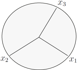
Figure 3: The first order Feynman diagram contributing to the scalar three-point function.

Thus, the 3-point function is a sum of two Feynman diagrams of the form shown in Fig. 3, with the lines denoting in the first case time ordered two-point functions, and in the second case, Wightman two-point functions. Using the known two-point functions gives

$$G_{F}^{(3)}(x_{1},x_{2},x_{3}) =-i\lambda\int d^{2}x\sqrt{|g|}\prod_{i=1}^{3}\frac{1}{\pi}\frac{z_{i}z}{-(\tau-\tau_{i})^{2}+z^{2}+i\epsilon}$$

$$+i\lambda\int d^{2}x\sqrt{|g|}\prod_{i=1}^{3}\frac{1}{\pi}\frac{z_{i}z}{-(\tau-\tau_{i})^{2}+z^{2}+i(\tau-\tau_{i})\epsilon}$$ (3.27)

The boundary three-point function in the "extrapolate" dictionary is given by

$$G_{F,\partial}^{(3)}(t_{1},t_{2},t_{3})=\lim_{z_{i}\rightarrow 0}(z_{1}z_{2}z_{3})^{-1}G^{(3)}(x_{1},x_{2},x_{3}).$$ (3.28)

Thus, we finally obtain the bulk 3-point function as the sum of the following integrals

$$G^{(3)}_{F,\partial}(\tau_{1},\tau_{2},\tau_{3}) =-i\lambda\int dzd\tau\,z\prod_{i=1}^{3}\frac{1}{\pi}\frac{1}{-(\tau-\tau_{i})^{2}+z^{2}+i\epsilon}$$

$$+i\lambda\int dzdt\,z\sqrt{|g|}\prod_{i=1}^{3}\frac{1}{\pi}\frac{1}{-(\tau-\tau_{i})^{2}+z^{2}+i(\tau-\tau_{i})\epsilon}$$ (3.29)

We will first compute the $\tau$ integrals, from the residues at the poles of the integrands. The Wightman two-point functions in the second line of (3.29) have poles at

$$\tau=\tau_{j}\pm z+i\epsilon.$$ (3.30)

As the poles are all located in the upper part of the complex $\tau$ plane, we can close the integral contour from below without encountering any poles. As the integrand vanishes as $\tau^{-6}$ at large $\tau$, the integral vanishes. Thus, the 3-point function reduces to the contribution from the time ordered 2-point functions, in the first line of (3.29). This is the expected result in the vacuum state, where the in-in and in-out formalisms are expected to agree. The time ordered two-point functions have poles at

$$\tau=\tau_{j}\pm z\pm i\epsilon.$$ (3.31)

Performing the $\tau$ integral by closing the integral contour from the upper half complex $\tau$ plane gives

$$G^{(3)}_{F,\partial}(\tau_{1},\tau_{2},\tau_{3})=-\frac{\lambda}{4\pi^{2}}\int_{0}^{\infty}dz\sum_{j=1}^{3}\prod_{k\neq j}\frac{1}{t_{jk}}\frac{1}{z+\frac{1}{2}(\tau_{jk}+i\epsilon)},$$ (3.32)

where $\tau_{jk}=\tau_{j}-\tau_{k}$. The $z$ integrals are now elementary and can be performed using the identity

$$\int_{0}^{\infty}\frac{dz}{(z+a)(z+b)}=\frac{1}{a-b}\log\Big{(}\frac{a}{b}\Big{)},$$ (3.33)

leading to

$$G^{(3)}_{F,\partial}(\tau_{1},\tau_{2},\tau_{3})=\frac{\lambda}{2\pi^{2}}\frac{1}{\tau_{12}\tau_{13}\tau_{23}}\log\Big{(}-1-i\epsilon\frac{\tau_{1}^{2}+\tau_{2}^{2}+\tau_{3}^{2}-\tau_{1}\tau_{2}-\tau_{1}\tau_{3}-\tau_{2}\tau_{3}}{\tau_{12}\tau_{13}\tau_{23}}\Big{)}.$$ (3.34)

Using $\log(-1-i\delta)=-i\pi\textrm{sign}(\delta)$ for $\delta\rightarrow 0$, gives finally

$$G^{(3)}_{F,\partial}(\tau_{1},\tau_{2},\tau_{3})=-i\frac{\lambda}{2\pi}\frac{1}{|\tau_{12}\tau_{23}\tau_{13}|}.$$ (3.35)

3.5 Vaidya 3-point functions

Next, consider the 3-point function in the AdS-Vaidya spacetime. Using the real time Schwinger-Keldysh formalism, with the above two-point functions gives the same integral expression as the ground state (3.27), but now in the barred coordinates. One difference to the vacuum case is that the integral over light-cone time now has an upper limit at $\bar{v}=2z_{H}$ due to the coordinate relation (3.4). It is easy to see that the integration region can be continued all the way to $\bar{v}=\infty$ without changing the value of the integral, as in this region, the integrands in the first and second lines of (3.27) identically cancel each other. This follows from unitarity, as the Schwinger-Keldysh contour can be extended forwards in time without changing the result for the correlation function. Thus, the same calculation of the integral in the vacuum 3-point function goes through and we obtain the near boundary 3-point function

$$G^{(3)}_{F}=-i\frac{\lambda}{2\pi}\frac{\bar{z}_{1}\bar{z}_{2}\bar{z}_{3}}{|\bar{\tau}_{12}\bar{\tau}_{23}\bar{\tau}_{13}|}.$$ (3.36)

Now depending on whether $\bar{\tau}_{j}$ is before or after the collapse, we get different results. When all of the points are in the region $\bar{\tau}_{j}<0$, we obtain the vacuum result. For $\bar{\tau}_{1}<0$, $\bar{\tau}_{2}<0$ and $\bar{\tau}_{3}>0$, we obtain using the extrapolate dictionary

$$G^{(3)}_{F,\partial}=-i\frac{\lambda}{2\pi}\frac{1}{\cosh^{2}\frac{t_{3}}{l}}\frac{1}{|(t_{1}-t_{2})(t_{1}-l\tanh\frac{t_{3}}{l})(t_{2}-l\tanh\frac{t_{3}}{l})|}.$$ (3.37)

On the other hand if two of the points $t_{2}$ and $t_{3}$ are located after the shell, we obtain

$$G^{(3)}_{F,\partial}=-i\frac{\lambda}{2\pi}\frac{1}{\cosh^{2}\frac{t_{3}}{l}\cosh^{2}\frac{t_{2}}{l}}\frac{1}{|(t_{1}-l\tanh\frac{t_{2}}{l})(t_{1}-l\tanh\frac{t_{3}}{l})(l\tanh\frac{t_{2}}{l}-l\tanh\frac{t_{3}}{l})|}.$$ (3.38)

And finally when all of the points are located after the shell, we obtain

$$G^{(3)}_{F,\partial} =-i\frac{\lambda}{2\pi}\frac{1}{\cosh^{2}\frac{t_{3}}{l}\cosh^{2}\frac{t_{2}}{l}\cosh^{2}\frac{t_{1}}{l}}\times$$

$$\times \frac{1}{|(l\tanh\frac{t_{1}}{l}-l\tanh\frac{t_{2}}{l})(l\tanh\frac{t_{1}}{l}-l\tanh\frac{t_{3}}{l})(l\tanh\frac{t_{2}}{l}-l\tanh\frac{t_{3}}{l})|}.$$ (3.39)

4 Four-point functions in finite temperature and with a quench

In conformal quantum mechanics, it is almost as straightforward to derive the non-equilibrium four-point functions as the three-point functions. For completeness, and for possible future reference, we end with this calculation. (For example, we expect that the structure of similar non-equilibrium 3- and 4-point functions in higher dimensional field theories reflects those of conformal quantum mechanics and can be reduced to them in an appropriate (equal space) limit. However, we expect the computation to be more involved in higher dimensions.) At zero temperature, for fields $\phi$ and $\tilde{\phi}$ with dimensions $\delta$ and $\tilde{\delta}$, respectively, the four-point function can be evaluated as (note, the corresponding expression in [15] contains a typo)

$$\mbox{}\langle t_{1}|\phi(t_{2})\tilde{\phi}(t_{3})|t_{4}\rangle=\frac{\Gamma(2r_{0})x^{r_{0}}\,_{2}F_{1}(\delta,\tilde{\delta};2r_{0};x)\langle 0|\phi(0)|0\rangle\langle 0|\tilde{\phi}(0)|0\rangle}{2^{\delta+\tilde{\delta}+2r_{0}}(t_{13})^{\tilde{\delta}-r_{0}}(t_{24})^{\delta-r_{0}}(t_{12})^{\delta+r_{0}}(t_{34})^{\tilde{\delta}+r_{0}}(t_{14})^{2r_{0}-\delta-\tilde{\delta}}}\ ,$$ (4.1)

where $t_{ij}=t_{i}-t_{j}$ and

$$x=\frac{t_{12}t_{34}}{t_{13}t_{24}},$$ (4.2)

is the conformally invariant ratio familiar from the usual conformal field theories. In the above, we have set the scaling parameter $a$ to unity. Here, the $x$ dependent factors remind us of the model dependent functions of 4-point functions in conformal field theories. It is noteworthy that the above expression can be obtained by using only a single conformal block. Now, we do the change of variables to the thermal coordinates.

$$x(\tau(t))=\frac{\sinh(\frac{t_{1}-t_{2}}{l})\sinh(\frac{t_{3}-t_{4}}{l})}{\sinh(\frac{t_{1}-t_{3}}{l})\sinh(\frac{t_{2}-t_{4}}{l})}\equiv x_{l}$$ (4.3)

and

$$\langle t_{1}|\phi(t_{2})\tilde{\phi}(t_{3})|t_{4}\rangle=$$

$$\frac{\langle 0|\phi(0)|0\rangle\langle 0|\tilde{\phi}(0)|0\rangle\Gamma(2r_{0})x_{l}^{r_{0}}\,{}_{2}F_{1}(\delta,\tilde{\delta};2r_{0};x_{l})2^{-\delta-\tilde{\delta}-2r_{0}}l^{-2r_{0}-\delta-\tilde{\delta}}}{\sinh(\frac{t_{13}}{l})^{\tilde{\delta}-r_{0}}\sinh(\frac{t_{24}}{l})^{\delta-r_{0}}\sinh(\frac{t_{12}}{l})^{\delta+r_{0}}\sinh(\frac{t_{34}}{l})^{\tilde{\delta}+r_{0}}\sinh(\frac{t_{14}}{l})^{2r_{0}-\delta-\tilde{\delta}}}\ .$$ (4.4)

Now for the real thing, thermalization. Now, we set the quench moment at $t=0$. Also, $t_{4}>0$ and $t_{1}<0$. We consider three different cases. First, $t_{2}<0,t_{3}<0$:

$$\langle t_{1}|\phi(t_{2})\tilde{\phi}(t_{3})|t_{4}\rangle=\frac{\langle 0|\phi(0)|0\rangle\langle 0|\tilde{\phi}(0)|0\rangle}{(t_{13})^{\tilde{\delta}-r_{0}}(t_{12})^{\delta+r_{0}}}\times$$ (4.5)

$$\mbox{}\frac{\Gamma(2r_{0})x_{q}^{r_{0}}\,{}_{2}F_{1}(\delta,\tilde{\delta};2r_{0};x_{q})2^{-\delta-\tilde{\delta}-2r_{0}}}{(t_{2}\sinh(\frac{t_{4}}{l})-l\sinh(\frac{t_{4}}{l}))^{\delta-r_{0}}(t_{3}\cosh(\frac{t_{4}}{l})-l\sinh(\frac{t_{4}}{l}))^{\tilde{\delta}+r_{0}}(t_{1}\cosh(\frac{t_{4}}{l})-l\sinh(\frac{t_{4}}{l}))^{2r_{0}-\delta-\tilde{\delta}}}\ ,$$

with

$$x_{q}\equiv\frac{t_{12}(\cosh(\frac{t_{4}}{l})t_{3}-l\sinh(\frac{t_{4}}{l}))}{t_{13}(\cosh(\frac{t_{4}}{l})t_{2}-l\sinh(\frac{t_{4}}{l}))}\ .$$ (4.6)

Then, $t_{2}<0,t_{3}>0$,

$$\langle t_{1}|\phi(t_{2})\tilde{\phi}(t_{3})|t_{4}\rangle=\frac{\langle 0|\phi(0)|0\rangle\langle 0|\tilde{\phi}(0)|0\rangle}{(t_{12})^{\delta+r_{0}}\sinh(\frac{t_{34}}{l})^{\tilde{\delta}+r_{0}}}\times$$ (4.7)

$$\frac{\Gamma(2r_{0})x_{q}^{r_{0}}\,{}_{2}F_{1}(\delta,\tilde{\delta};2r_{0};x_{q})2^{-\delta-\tilde{\delta}-2r_{0}}l^{-\tilde{\delta}-r_{0}}}{(t_{1}\cosh(\frac{t_{3}}{l})-l\sinh(\frac{t_{3}}{l}))^{\tilde{\delta}-r_{0}}(t_{2}\sinh(\frac{t_{4}}{l})-l\sinh(\frac{t_{4}}{l}))^{\delta-r_{0}}(t_{1}\cosh(\frac{t_{4}}{l})-l\sinh(\frac{t_{4}}{l}))^{2r_{0}-\delta-\tilde{\delta}}}\ ,$$

with

$$x_{q}\equiv\frac{lt_{12}\sinh(\frac{t_{34}}{l})}{(\cosh(\frac{t_{3}}{l})t_{1}-l\sinh(\frac{t_{3}}{l}))(\cosh(\frac{t_{4}}{l})t_{2}-l\sinh(\frac{t_{4}}{l}))}\ .$$ (4.8)

Finally, when both $t_{2},t_{3}>0$, we have

$$\langle t_{1}|\phi(t_{2})\tilde{\phi}(t_{3})|t_{4}\rangle=\frac{\langle 0|\phi(0)|0\rangle\langle 0|\tilde{\phi}(0)|0\rangle}{(t_{1}\cosh(\frac{t_{2}}{l})-l\sinh(\frac{t_{2}}{l}))^{\delta+r_{0}}(t_{1}\cosh(\frac{t_{3}}{l})-l\sinh(\frac{t_{3}}{l}))^{\tilde{\delta}-r_{0}}}\times$$ (4.9)

$$\frac{\Gamma(2r_{0})x_{q}^{r_{0}}\,{}_{2}F_{1}(\delta,\tilde{\delta};2r_{0};x_{q})2^{-\delta-\tilde{\delta}-2r_{0}}l^{-\tilde{\delta}-\delta}}{(t_{1}\cosh(\frac{t_{4}}{l})-l\sinh(\frac{t_{4}}{l}))^{2r_{0}-\delta-\tilde{\delta}}\sinh(\frac{t_{34}}{l})^{\tilde{\delta}+r_{0}}\sinh(\frac{t_{24}}{l})^{\delta-r_{0}}}\ ,$$

where

$$x_{q}\equiv\frac{(t_{1}\cosh(\frac{t_{2}}{l})-l\sinh(\frac{t_{2}}{l}))\sinh(\frac{t_{34}}{l})}{(t_{1}\cosh(\frac{t_{3}}{l})-l\sinh(\frac{t_{3}}{l}))\sinh(\frac{t_{24}}{l})}\ .$$ (4.10)

The results are of course what one expects, the structure of the four (and three)-point functions change in a systematic way at different points of time with respect to the quench moment.

For further study, it would be interesting to include the backreaction corrections to the 3-point functions [3], or to study how the 3- and 4-point functions in CQM are recovered from higher dimensions. The non-equilibrium 2-point function agrees with the equal space limit of the 2-point function in 1+1 dimensions, in the limit of large operator dimension when the 2-point function is well approximated by the geodesic approach. The analytical results for the correlation functions would be interesting to compare with the equal space limits of $d$+1 correlation functions for $d>1$, because the blackening factor in the bulk black hole metric is dimension dependent. It would also be interesting to see how the (semiclassical) limit of 4-point functions computed in higher dimensions [12, 13, 14] reduce to the 4-point function in CQM.

Acknowledgments

JJ and EKV are in part supported by the Academy of Finland grant no 1268023. JJ is also in part supported by the U. Helsinki Graduate School PAPU. The research of VK was supported by the European Research Council under the European Union’s Seventh Framework Programme (ERC Grant agreement 307955). EKV also thanks the Galileo Galilei Institute for its hospitality and partial support, and EKV and JJ thank the [Department of Energy’s] Institute for Nuclear Theory at the University of Washington for its hospitality and the Department of Energy for partial support, during the completion of this work.

Appendix

We motivate the definition $O_{Vaidya}(t)$ in (3.12) by checking that the time evolution of the state $|\tau\rangle=O_{P}(\tau)|0\rangle$ connects to that of $|t\rangle=O_{BH}(t)|0\rangle$ after the quench.

Recall that

$$|\tau\rangle=O_{P}(\tau)|0\rangle=e^{i\tau H_{P}}e^{aH_{P}}|0\rangle$$ (4.11)

where the second exponential prepares the state $|\tau=0\rangle$ and the first factor $e^{i\tau H_{P}}$ continues the time evolution (also to earlier times). The state $|\tau=0\rangle=|t=0\rangle$ at the quench. After the quench, the time evolution continues with the new time translation generator $H_{BH}$, so it should evaluate to the state

$$|t\rangle^{\prime}\equiv O_{BH}(t)|0\rangle=e^{itH_{BH}}e^{aH_{P}}|0\rangle\ .$$ (4.12)

On the other hand, we had defined the state $|t\rangle$ to be

$$|t\rangle=\left(\frac{d\tau}{dt}\right)^{r_{0}}|\tau=\tau(t)\rangle=\left[\cosh(t/l)\right]^{-2r_{0}}|\tau=l\tanh(t/l)\rangle$$ (4.13)

where $l=2u_{H}$. Thus, we need to show that the two states are the same, $|t\rangle^{\prime}=|t\rangle$. To establish that, we study how they time evolve. On one hand,

$$-i\partial_{t}|t\rangle = \left[i\frac{2r_{0}}{l}\sinh(t/l)[\cosh(t/l)]^{-1}+\cosh^{-2}(t/l)H_{P}\right]|t\rangle$$ (4.14)

$$= \cosh^{-2}(t/l)\left[H_{P}+i\frac{2r_{0}}{l}\cosh(t/l)\sinh(t/l)\right]|t\rangle.$$

On the other hand,

$$-i\partial_{t}|t\rangle^{\prime}=H_{BH}|t\rangle^{\prime}=(H_{P}+\gamma K)|t\rangle^{\prime}\ ,$$ (4.15)

where $\gamma=-1/l^{2}$. We then show that the above two first order equations are in fact identical. Since the initial state $|t=\tau=0\rangle=e^{aH_{p}}|0\rangle$ is the same, that ensures that $|t\rangle^{\prime}=|t\rangle$.

Starting from

$$K|t\rangle = -i\left(\tau^{2}\partial_{\tau}+2r_{0}\tau\right)|t\rangle=\left(\tau^{2}H_{P}-i2r_{0}\tau\right)|t\rangle$$ (4.16)

$$= \left[\frac{1}{\gamma}\left(\cosh^{-2}(t/l)-1\right)H_{P}+\frac{i2r_{0}}{\gamma l}\tanh(t/l)\right]|t\rangle$$

we obtain

$$(H_{P}+\gamma K)|t\rangle=\left[\cosh^{-2}(t/l)H_{P}+\frac{i2r_{0}}{l}\tanh(t/l)\right]|t\rangle=-i\partial_{t}|t\rangle$$ (4.17)

so that $|t\rangle$ indeed satisfies the same first order equation as $|t\rangle^{\prime}$.

References

- [1] V. de Alfaro, S. Fubini and G. Furlan, “Conformal Invariance in Quantum Mechanics,” Nuovo Cim. A 34, 569 (1976).
- [2] J. M. Maldacena, J. Michelson and A. Strominger, “Anti-de Sitter fragmentation,” JHEP 9902, 011 (1999) [hep-th/9812073].
- [3] A. Almheiri and J. Polchinski, “Models of AdS2 Backreaction and Holography,” arXiv:1402.6334 [hep-th].
- [4] T. Banks, M. R. Douglas, G. T. Horowitz and E. J. Martinec, “AdS dynamics from conformal field theory,” hep-th/9808016.
- [5] V. E. Hubeny, M. Rangamani and T. Takayanagi, “A Covariant holographic entanglement entropy proposal,” JHEP 0707, 062 (2007) [arXiv:0705.0016 [hep-th]].
- [6] J. Abajo-Arrastia, J. Aparicio and E. Lopez, “Holographic Evolution of Entanglement Entropy,” JHEP 1011, 149 (2010) [arXiv:1006.4090 [hep-th]].
- [7] T. Albash and C. V. Johnson, “Evolution of Holographic Entanglement Entropy after Thermal and Electromagnetic Quenches,” New J. Phys. 13, 045017 (2011) [arXiv:1008.3027 [hep-th]].
- [8] V. Balasubramanian et al., “Thermalization of Strongly Coupled Field Theories,” Phys. Rev. Lett. 106, 191601 (2011) [arXiv:1012.4753 [hep-th]].
- [9] V. Balasubramanian et al., “Holographic Thermalization,” Phys. Rev. D 84, 026010 (2011) [arXiv:1103.2683 [hep-th]].
- [10] C. Chamon, R. Jackiw, S. Y. Pi and L. Santos, “Conformal quantum mechanics as the CFT1 dual to AdS2,” Phys. Lett. B 701, 503 (2011) [arXiv:1106.0726 [hep-th]].
- [11] P. Arnold and D. Vaman, JHEP 1010, 099 (2010) doi:10.1007/JHEP10(2010)099 [arXiv:1008.4023 [hep-th]]; P. Arnold and D. Vaman, JHEP 1104 (2011) 027 doi:10.1007/JHEP04(2011)027 [arXiv:1101.2689 [hep-th]]; P. Arnold and D. Vaman, J. Phys. G 38, 124175 (2011) doi:10.1088/0954-3899/38/12/124175 [arXiv:1106.1680 [hep-th]]; P. Arnold, D. Vaman, C. Wu and W. Xiao, JHEP 1110, 033 (2011) doi:10.1007/JHEP10(2011)033 [arXiv:1105.4645 [hep-th]]; O. Saremi and K. A. Sohrabi, JHEP 1111, 147 (2011) doi:10.1007/JHEP11(2011)147 [arXiv:1105.4870 [hep-th]].
- [12] A. L. Fitzpatrick, J. Kaplan and M. T. Walters, “Universality of Long-Distance AdS Physics from the CFT Bootstrap,” JHEP 1408, 145 (2014) [arXiv:1403.6829 [hep-th]].
- [13] C. T. Asplund, A. Bernamonti, F. Galli and T. Hartman, “Holographic Entanglement Entropy from 2d CFT: Heavy States and Local Quenches,” JHEP 1502, 171 (2015) [arXiv:1410.1392 [hep-th]].
- [14] E. Hijano, P. Kraus and R. Snively, “Worldline approach to semi-classical conformal blocks,” JHEP 1507, 131 (2015) [arXiv:1501.02260 [hep-th]].
- [15] R. Jackiw and S.-Y. Pi, “Conformal Blocks for the 4-Point Function in Conformal Quantum Mechanics,” Phys. Rev. D 86, 045017 (2012) [Phys. Rev. D 86, 089905 (2012)] [arXiv:1205.0443 [hep-th]].
- [16] D. Anninos, S. A. Hartnoll and D. M. Hofman, “Static Patch Solipsism: Conformal Symmetry of the de Sitter Worldline,” Class. Quant. Grav. 29, 075002 (2012) [arXiv:1109.4942 [hep-th]].
- [17] R. Nakayama, “The World-Line Quantum Mechanics Model at Finite Temperature which is Dual to the Static Patch Observer in de Sitter Space,” Prog. Theor. Phys. 127, 393 (2012) [arXiv:1112.1267 [hep-th]].
- [18] M. Spradlin and A. Stromiger, “Vacuum States for AdS2 Black Holes,” JHEP 9911, 021 (1999) [hep-th/9904143].
- [19] P. M. Ho, JHEP 0405, 008 (2004) doi:10.1088/1126-6708/2004/05/008 [hep-th/0401167].
- [20] H. Ebrahim and M. Headrick, “Instantaneous Thermalization in Holographic Plasmas,” arXiv:1010.5443 [hep-th].
- [21] V. Keranen and P. Kleinert, “Non-equilibrium scalar two point functions in AdS/CFT,” JHEP 1504, 119 (2015) [arXiv:1412.2806 [hep-th]].
- [22] V. Balasubramanian, A. Bernamonti, B. Craps, V. Keränen, E. Keski-Vakkuri, B. Müller, L. Thorlacius and J. Vanhoof, “Thermalization of the spectral function in strongly coupled two dimensional conformal field theories,” JHEP 1304, 069 (2013) [arXiv:1212.6066 [hep-th]].
- [23] P. Calabrese and J. Cardy, “Entanglement entropy and conformal field theory,” J. Phys. A 42, 504005 (2009) [arXiv:0905.4013 [cond-mat.stat-mech]].