Restoring broken entanglement by separable correlations

Abstract

We consider two bosonic Gaussian channels whose thermal noise is strong enough to break bipartite entanglement. In this scenario, we show how the presence of separable correlations between the two channels is able to restore the broken entanglement. This reactivation occurs not only in a scheme of direct distribution, where a third party (Charlie) broadcasts entangled states to remote parties (Alice and Bob), but also in a configuration of indirect distribution which is based on entanglement swapping. In both schemes, the amount of entanglement remotely activated can be large enough to be distilled by one-way distillation protocols.

Entanglement is a fundamental physical resource in quantum information and computation. Once two parties, say Alice and Bob, share a suitable amount of entanglement, they can implement a variety of powerful protocols NielsenBook ; Mwilde . In a scheme of direct distribution, there is a middle station (Charlie) possessing a bipartite system in an entangled state; one subsystem is sent to Alice and the other to Bob. Alternatively, in a scheme of indirect distribution, known as entanglement swapping, the distribution is mediated by a measurement process. Here Alice and Bob each has a bipartite system prepared in an entangled state. One subsystem is retained while the other is sent to Charlie. At his station, Charlie detects the two incoming subsystems by performing a suitable Bell measurement and communicates the classical outcome back to Alice and Bob. As a result of this process, the two subsystems retained by the remote parties are projected onto an entangled state.

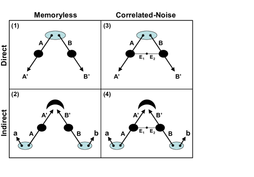
Figure 1: Direct and indirect schemes for entanglement distribution in memoryless and correlated-noise environments. Charlie is the middle station transmitting to or receiving systems from Alice (left station) and Bob (right station). Ellipses represent entangled states, black-circles represent channels, and detectors are Bell measurements. (1) Direct distribution in a memoryless environment. If the individual channels are EB, then no distribution of entanglement is possile. We have $A|B^{\prime}$ and $A^{\prime}|B$ which implies $A^{\prime}|B^{\prime}$. (2) Entanglement swapping in a memoryless environment. We have that $a|A^{\prime}$ and $B^{\prime}|b$ implies $a|b$. (3) Direct distribution in a correlated environment. Despite $A|B^{\prime}$ and $A^{\prime}|B$ we have that $A^{\prime}-B^{\prime}$ is possible. Surprisingly, this can be realized by a separable environment. (4) Entanglement swapping in a correlated environment. Despite $a|A^{\prime}$ and $B^{\prime}|b$ we have that $a-b$ is possible. Surprisingly, this is realizable by a separable environment.

In both configurations, entanglement distribution is possible as long as the action of the environment is not too strong. When decoherence is strong enough to destroy any input entanglement, the environment results into an entanglement breaking (EB) channel EBchannels ; HolevoEB . By definition, a quantum channel $\mathcal{E}$ is EB when its local action on one part of a bipartite state always results into a separable output state. In other words, given two systems, $A$ and $B$, in an arbitrary bipartite state $\rho_{AB}$, the output state $\rho_{AB^{\prime}}=(\mathcal{I}_{A}\otimes\mathcal{E}_{B})(\rho_{AB})$ is always separable, where $\mathcal{I}_{A}$ is the identity channel applied to system $A$ and $\mathcal{E}_{B}$ is the EB channel applied to system $B$. Thus, if the input systems $A$ and $B$ were initially entangled (here denoted by the notation $A-B$), the output systems $A$ and $B^{\prime}$ are separable (here denoted by the notation $A|B^{\prime}$).

The standard model of decoherence is assumed to be Markovian, where the travelling systems are subject to memoryless channels. For instance, consider the case of direct distribution depicted in the panel (1) of Fig. 1. In the standard Markovian description, the entangled state $\rho_{AB}$ of the input systems $A$ and $B$ is subject to a tensor product of channels $\mathcal{E}_{A}\otimes\mathcal{E}_{B}$. In this case, there is clearly no way to distribute entanglement if both $\mathcal{E}_{A}$ and $\mathcal{E}_{B}$ are EB channels. Suppose that Charlie tries to share entanglement with one of the remote parties by sending one of the two systems while keeping the other (one-system transmission). For instance, Charlie may keep system $A$ while transmitting system $B$ to Bob. The action of $\mathcal{I}_{A}\otimes\mathcal{E}_{B}$ destroys the initial entanglement, so that systems $A$ (kept) and $B^{\prime}$ (transmitted) are separable ($A|B^{\prime}$). Symmetrically, the action of $\mathcal{E}_{A}\otimes\mathcal{I}_{B}$ destroys the entanglement between system $A^{\prime}$ (transmitted) and system $B$ (kept), i.e., we have $A^{\prime}|B$. Then suppose that Charlie sends both his systems to Alice and Bob (two-system transmission). This strategy will also fail since the joint action of the two EB channels is given by the tensor product $\mathcal{E}_{A}\otimes\mathcal{E}_{B}=(\mathcal{E}_{A}\otimes\mathcal{I}_{B})(\mathcal{I}_{A}\otimes\mathcal{E}_{B})$. In other words, since we have one-system EB ($A|B^{\prime}$ and $A^{\prime}|B$) then we must have two-system EB ($A^{\prime}|B^{\prime}$).

The previous reasoning can be extended to the case of indirect distribution as shown in panel (2) of Fig. 1 involving a Bell measurement by Charlie. Since the environment is memoryless ($\mathcal{E}_{A}\otimes\mathcal{E}_{B}$), we have that the absence of entanglement before the Bell measurement ($a|A^{\prime}$ and $B^{\prime}|b$) is a sufficient condition for the swapping protocol to fail, i.e., the remote systems $a$ and $b$ remains separable ($a|b$). Similarly to the previous case, if one-system transmission does not distribute entanglement, then two-system transmission cannot lead to entanglement generation via the swapping protocol.

Here we discuss how the previous implications for direct and indirect distribution of entanglement are false in the presence of a correlated-noise environment: Two-system transmission can successfully distribute entanglement despite one-system transmission being subject to EB. In other words, by combining two EB channels into a joint suitably-correlated environment, we can reactivate the distribution of entanglement. We will show the physical conditions under which the environmental correlations are able to trigger the reactivation, therefore “breaking entanglement-breaking”. The most remarkable finding is that we do not need to consider an entangled state for the environment: The injection of separable correlations from the environment is sufficient for the restoration.

To better clarify these points, consider the schemes of direct and indirect distribution in the presence of a correlated-noise environment. In the scheme of direct distribution shown in panel (3) of Fig. 1, an input entangled state $\rho_{AB}$ is jointly transformed into an output state $\rho_{A^{\prime}B^{\prime}}=\mathcal{E}_{AB}(\rho_{AB})$. We assume that the dilation of the composite channel $\mathcal{E}_{AB}$ is realized by introducing a two-system environment, $E_{1}$ and $E_{2}$, in a bipartite state $\rho_{E_{1}E_{2}}$, which interacts with the incoming systems via two unitaries $U_{AE_{1}}$ (transforming $A$ and $E_{1}$) and $U_{BE_{2}}$ (transforming $B$ and $E_{2}$). In other words, the output state can be written in the form

$$\rho_{A^{\prime}B^{\prime}} =\mathrm{Tr}_{E_{1}E_{2}}[(U_{AE_{1}}\otimes U_{BE_{2}})$$

$$\times(\rho_{AB}\otimes\rho_{E_{1}E_{2}})(U_{AE_{1}}^{\dagger}\otimes U_{BE_{2}}^{\dagger})].$$ (1)

If the environmental state is not tensor product, i.e., $\rho_{E_{1}E_{2}}\neq\rho_{E_{1}}\otimes\rho_{E_{2}}$, then the composite channel cannot be decomposed into memoryless channels, i.e., $\mathcal{E}_{AB}\neq\mathcal{E}_{A}\otimes\mathcal{E}_{B}$. In any case, from the dilation given in Eq. (1), we can always define the reduced channels, $\mathcal{E}_{A}$ and $\mathcal{E}_{B}$, acting on the individual systems. For instance, if only system $B$ is transmitted, then we have the evolved state

$$\rho_{AB^{\prime}} =(\mathcal{I}_{A}\otimes\mathcal{E}_{B})(\rho_{AB})$$

$$=\mathrm{Tr}_{E_{2}}[(I_{A}\otimes U_{BE_{2}})\rho_{AB}\otimes\rho_{E_{2}}(I_{A}\otimes U_{BE_{2}}^{\dagger})],$$ (2)

where $\rho_{E_{2}}=\mathrm{Tr}_{E_{1}}(\rho_{E_{1}E_{2}})$. A similar formula holds for the evolution of the other system $\rho_{A^{\prime}B}=(\mathcal{E}_{A}\otimes\mathcal{I}_{B})(\rho_{AB})$.

Now, assuming that $\mathcal{I}_{A}\otimes\mathcal{E}_{B}$ and $\mathcal{E}_{A}\otimes\mathcal{I}_{B}$ are EB channels (so that $A|B^{\prime}$ and $B|A^{\prime}$), the composite channel $\mathcal{E}_{AB}$ can still preserve entanglement (so that $A^{\prime}-B^{\prime}$ is possible). In other words, we have a paradoxical situation where Charlie is not able to share entanglement with Alice or Bob, but still can distribute entanglement to them. This is clearly an effect of the injected correlations coming from the environmental state $\rho_{E_{1}E_{2}}$. As mentioned earlier, our main finding is that these correlations do not need to be strong: Entanglement distribution can be activated by separable correlations, i.e., by an environment which is in a separable state $\rho_{E_{1}E_{2}}$.

This effect of reactivation can also be extended to entanglement distillation, which typically requires stronger conditions than entanglement distribution (demanded by the existence of effective distillation protocols). Despite the individual channels are EB, their combination into a separable environment enables Charlie to distribute distillable entanglement to Alice and Bob. This is easy to prove for an environment with finite memory, which can be decomposed as $\mathcal{E}_{AB}\otimes\mathcal{E}_{AB}\otimes\ldots$

In our investigation, we also consider the case of entanglement swapping in a correlated-noise environment as depicted in panel (4) of Fig. 1. Here Alice and Bob have two entangled states, $\rho_{aA}$ and $\rho_{Bb}$, respectively. Systems $a$ and $b$ are retained, while systems $A$ and $B$ are transmitted to Charlie, therefore undergoing the joint quantum channel $\mathcal{E}_{AB}$. Before the Bell measurement, the global state is described by

$$\rho_{aA^{\prime}B^{\prime}b} =(\mathcal{I}_{a}\otimes\mathcal{E}_{AB}\otimes\mathcal{I}_{b})(\rho_{aA}\otimes\rho_{Bb})$$

$$=\mathrm{Tr}_{E_{1}E_{2}}[U(\rho_{aA}\otimes\rho_{E_{1}E_{2}}\otimes\rho_{Bb})U^{\dagger}]~{},$$ (3)

where $U=I_{a}\otimes U_{AE_{1}}\otimes U_{E_{2}B}\otimes I_{b}$.

As before, we consider the case where the reduced channels, $\mathcal{E}_{A}$ and $\mathcal{E}_{B}$, are EB channels, so that no entanglement survives before the Bell measurement ($a|A^{\prime}$ and $B^{\prime}|b$). If the environment has no memory ($\rho_{E_{1}E_{2}}=\rho_{E_{1}}\otimes\rho_{E_{2}}$) there is no way to distribute entanglement to Alice and Bob ($a|b$). By contrast, if the environment has memory ($\rho_{E_{1}E_{2}}\neq\rho_{E_{1}}\otimes\rho_{E_{2}}$), then entanglement distribution is possible ($a-b$) and this distribution can be activated by a separable environmental state $\rho_{E_{1}E_{2}}$. Thus, we have the paradoxical situation where no bipartite entanglement survives at Charlie’s station ($a|A^{\prime}$ and $B^{\prime}|b$), but still the swapping protocol is able to generate remote entanglement at Alice’s and Bob’s stations ($a-b$) thanks to the separable correlations injected by the environment. As before, these separable correlations can be strong enough to distribute distillable entanglement to the remote parties.

The environmental reactivation of entanglement distribution can be proven NJP for quantum systems with Hilbert spaces of any dimension, both finite (discrete-variable systems) and infinite (continuous-variable systems BraREV ; BraREV2 ; RMP ). We remark that the phenomenon of reactivation in direct distribution is not surprising in specific lossless scenarios where the environment is “twirling”, i.e., a classical mixture of operators of the type $U\otimes U$ or $U\otimes U^{\ast}$, with $U$ being a unitary NJP . In this case, it is easy to find a fixed point in the joint map of the environment, so that a state can be perfectly distributed, despite the fact that the local (single-system) channels may become entanglement breaking NJP . In discrete variables with Hilbert space dimensionality $d\geq 2$, these fixed points are the multi-dimensional Werner states Werner (invariant under $U\otimes U$-twirling) and the multi-dimensional isotropic states HOROs (invariant under $U\otimes U^{\ast}$-twirling). Similarly, one can consider continuous-variable Werner states which are invariant under anti-correlated phase-space rotations (non-Gaussian twirlings) NJP . However, all these cases are artificial since they are associated with lossless environments. The phenomenon of reactivation becomes non-trivial in the presence of loss as typical for continuous variable systems in realistic Gaussian environments.

In the configuration of indirect distribution, we can also find simple examples of reactivation with discrete variable systems (in particular, qubits) when the environment is lossless and $U\otimes U^{\ast}$-twirling. Suppose that $\rho_{aA}$ and $\rho_{bB}$ are Bell pairs, e.g., singlet states

$$\left|-\right\rangle=\frac{1}{\sqrt{2}}\left(\left|0,1\right\rangle-\left|1,0\right\rangle\right)~{}.$$ (4)

Then suppose that qubits $A$ and $B$ are subject to twirling, which means that $\rho_{AB}$ is transformed as

$$\rho_{A^{\prime}B^{\prime}}=\int dU~{}(U\otimes U^{\ast})~{}\rho_{AB}~{}(U\otimes U^{\ast})^{\dagger}~{},$$ (5)

where the integral is over the entire unitary group $\mathcal{U}(2)$ acting on the bi-dimensional Hilbert space and $dU$ is the Haar measure. Now the application of a Bell detection on the output qubits $A^{\prime}$ and $B^{\prime}$ has the effect to cancel the environmental noise. In fact, one can easily check that the output state of $a$ and $b$ will be projected onto a singlet state up to a Pauli operator, which is compensated via the communication of the Bell outcome. Again, the phenomenon becomes non-trivial when more realistic environments are taken into account, in particular, lossy environments as typical for continuous-variable systems.

For this reason we discuss here the reactivation phenomenon using continuous-variable systems. In particular, we consider the bosonic modes of the electromagnetic field. The input modes are prepared in Gaussian states with Einstein-Podolsky-Rosen (EPR) correlations RMP ; EPR , which are the most typical form of continuous variable entanglement. These modes are then assumed to evolve under the action of a lossy Gaussian environment. This type of environment is modelled by two beam splitters which mix the travelling modes, $A$ and $B$, with two environmental modes, $E_{1}$ and $E_{2}$, prepared in a bipartite Gaussian state $\rho_{E_{1}E_{2}}$ (separable or entangled). The reduced channels, $\mathcal{E}_{A}$ and $\mathcal{E}_{B}$, are two lossy channels whose transmissivities and thermal noises are such to make them EB channels. To achieve simple analytical results, in this manuscript we only consider the limit of large entanglement for the input states.

The paper is structured as follows. In Sec. I we characterize the basic model of correlated Gaussian environment, which directly generalizes the standard model of thermal-loss environment. We identify the physical conditions under which the correlated Gaussian environment is separable or entangled. In Sec. II, we study the direct distribution of entanglement in the presence of the correlated Gaussian environment and assuming the condition of one-system EB. We provide the regimes of parameters under which remote entanglement is activated by the environmental correlations (in particular, separable correlations) and the stronger regimes where the generated remote entanglement is also distillable. This part is a review of results already known in the literature NJP . Then, in Sec. III, we generalize the theory of entanglement swapping to the correlated Gaussian environment. We consider swapping and distillation of entanglement, finding the regimes of parameters where these tasks are successful despite the EB condition. Finally, Sec. IV is for conclusion and discussion.

I Correlated Gaussian environment

We consider two beam splitters (with transmissivity $\tau$) which combine modes $A$ and $B$ with two environmental modes, $E_{1}$ and $E_{2}$, respectively. These ancillary modes are in a zero-mean Gaussian state $\rho_{E_{1}E_{2}}$ symmetric under $E_{1}$-$E_{2}$ permutation. In the memoryless model, the environmental state is tensor-product $\rho_{E_{1}E_{2}}=\rho\otimes\rho$, meaning that $E_{1}$ and $E_{2}$ are fully independent. In particular, $\rho$ is a thermal state with covariance matrix (CM) $\omega\mathbf{I}$, where the noise variance $\omega=2\bar{n}+1$ quantifies the mean number of thermal photons $\bar{n}$ entering the beam splitter. Each interaction is then equivalent to a lossy channel with transmissivity $\tau$ and thermal noise $\omega$.

Figure 2: Left. Correlated Gaussian environment, with losses $\tau$, thermal noise $\omega$ and correlations $\mathbf{G}$. The state of the environment $E_{1}$ and $E_{2}$ can be separable or entangled. Right. Correlation plane $(g,g^{\prime})$ for the Gaussian environment, corresponding to thermal noise $\omega=2$. The black area identifies forbidden environments (correlations are too strong to be compatible with quantum mechanics). White area identifies physical environments, i.e., the subset of points which satisfy the bona-fide conditions of Eq. (8). Whitin this area, the inner region labbeled by S identifies separable environments, while the two outer regions identify entangled environments. Figures adapted from Ref. NJP under a CC BY 3.0 licence (http://creativecommons.org/licenses/by/3.0/).

This Gaussian process can be generalized to include the presence of correlations between the environmental modes as depicted in the right panel of Fig. 2. The simplest extension of the model consists of taking the ancillary modes, $E_{1}$ and $E_{2}$, in a zero-mean Gaussian state $\rho_{E_{1}E_{2}}$ with CM given by the symmetric normal form

$$\mathbf{V}_{E_{1}E_{2}}(\omega,g,g^{\prime})=\left(\begin{array}[c]{cc}\omega\mathbf{I}&\mathbf{G}\\ \mathbf{G}&\omega\mathbf{I}\end{array}\right)~{},$$ (6)

where $\omega\geq 1$ is the thermal noise variance associated with each ancilla, and the off-diagonal block

$$\mathbf{G=}\left(\begin{array}[c]{cc}g&\\ &g^{\prime}\end{array}\right)~{},$$ (7)

accounts for the correlations between the ancillas. This type of environment can be separable or entangled (conditions for separability will be given afterwards).

It is clear that, when we consider the two interactions $A-E_{1}$ and $B-E_{2}$ separately, the environmental correlations are washed away. In fact, by tracing out $E_{2}$, we are left with mode $E_{1}$ in a thermal state ($\mathbf{V}_{E_{1}}=\omega\mathbf{I}$) which is combined with mode $A$ via the beam-splitter. In other words, we have again a lossy channel with transmissivity $\tau$ and thermal noise $\omega$. The scenario is identical for the other mode $B$ when we trace out $E_{1}$. However, when we consider the joint action of the two environmental modes, the correlation block $\mathbf{G}$ comes into play and the global dynamics of the two travelling modes becomes completely different from the standard memoryless scenario.

Before studying the system dynamics and the corresponding evolution of entanglement, we need to characterize the correlation block $\mathbf{G}$ more precisely. In fact, the two correlation parameters, $g$ and $g^{\prime}$, cannot be completely arbitrary but must satisfy specific physical constraints. These parameters must vary within ranges which make the CM of Eq. (6) a bona-fide quantum CM. Given an arbitrary value of the thermal noise $\omega\geq 1$, the correlation parameters must satisfy the following three bona-fide conditions TwomodePRA ; NJP

$$|g|<\omega,~{}~{}~{}|g^{\prime}|<\omega,~{}~{}~{}\omega^{2}+gg^{\prime}-1\geq\omega\left|g+g^{\prime}\right|.$$ (8)

I.1 Separability properties

Once we have clarified the bona-fide conditions for the environment, the next step is to characterize its separability properties. For this aim, we compute the smallest partially-transposed symplectic (PTS) eigenvalue $\varepsilon$ associated with the CM $\mathbf{V}_{E_{1}E_{2}}$. For Gaussian states, this eigenvalue represents an entanglement monotone which is equivalent to the log-negativity logNEG1 ; logNEG2 ; logNEG3 $\mathcal{E}=\max\left\{0,-\log\varepsilon\right\}$. After simple algebra, we get NJP

$$\varepsilon=\sqrt{\omega^{2}-gg^{\prime}-\omega|g-g^{\prime}|}~{}.$$ (9)

Provided that the conditions of Eq. (8) are satisfied, the separability condition $\varepsilon\geq 1$ is equivalent to

$$\omega^{2}-gg^{\prime}-1\geq\omega|g-g^{\prime}|~{}.$$ (10)

To visualize the structure of the environment, we provide a numerical example in Fig. 2. In the right panel of this figure, we consider the correlation plane which is spanned by the two parameters $g$ and $g^{\prime}$. For a given value of the thermal noise $\omega$, we identify the subset of points which satisfy the bona-fide conditions of Eq. (8). This subset corresponds to the white area in the figure. Within this area, we then characterize the regions which correspond to separable environments (area labelled by S) and entangled environments (areas labelled by E).

II Direct distribution of entanglement in a correlated Gaussian environment

Let us study the system dynamics and the entanglement propagation in the presence of a correlated Gaussian environment, reviewing some key results from the literature NJP . Suppose that Charlie has an entanglement source described by an EPR state $\rho_{AB}$ with CM

$$\mathbf{V}(\mu)=\left(\begin{array}[c]{cc}\mu\mathbf{I}&\mu^{\prime}\mathbf{Z}\\ \mu^{\prime}\mathbf{Z}&\mu\mathbf{I}\end{array}\right)~{},$$ (11)

where $\mu\geq 1$, $\mu^{\prime}:=\sqrt{\mu^{2}-1}$, and $\mathbf{Z}$ is the reflection matrix

$$\mathbf{Z}:=\left(\begin{array}[c]{cc}1&\\ &-1\end{array}\right)~{}.$$ (12)

We may consider the different scenarios depicted in the three panels of Fig. 3. Charlie may attempt to distribute entanglement to Alice and Bob as shown in Fig. 3(1), or he may try to share entanglement with one of the remote parties, as shown in Figs. 3(2) and (3).

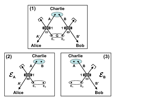
Figure 3: Scenarios for direct distribution of entanglement. (1) Charlie has two modes $A$ and $B$ prepared in an EPR state $\rho_{AB}$. In order to distribute entanglement to the remote parties, Charlie transmits the two modes through the correlated Gaussian environment characterized by transmissivity $\tau$, thermal noise $\omega$ and correlations $\mathbf{G}$. (2) Charlie aims to share entanglement with Alice. He then keeps mode $B$ while sending mode $A$ to Alice through the lossy channel $\mathcal{E}_{A}$. (3)  Charlie aims to share entanglement with Bob. He then keeps mode $A$ while sending mode $B$ to Bob through the lossy channel $\mathcal{E}_{B}$.

Let us start considering the scenario where Charlie aims to share entanglement with one of the remote parties (one-mode transmission). In particular, suppose that Charlie wants to share entanglement with Bob (by symmetry the derivation is the same if we consider Alice). For sharing entanglement, Charlie keeps mode $A$ while sending mode $B$ to Bob as shown in Fig. 3(3). The action of the environment is therefore reduced to $\mathcal{I}_{A}\otimes\mathcal{E}_{B}$, where $\mathcal{E}_{B}$ is a lossy channel applied to mode $B$. It is easy to check NJP that the output state $\rho_{AB^{\prime}}$, shared by Charlie and Bob, is Gaussian with zero mean and CM

$$\mathbf{V}_{AB^{\prime}}=\left(\begin{array}[c]{cc}\mu\mathbf{I}&\mu^{\prime}\sqrt{\tau}\mathbf{Z}\\ \mu^{\prime}\sqrt{\tau}\mathbf{Z}&x\mathbf{I}\end{array}\right),$$ (13)

where

$$x:=\tau\mu+(1-\tau)\omega~{}.$$ (14)

Remarkably, we can compute closed analytical formulas in the limit of large $\mu$, i.e., large input entanglement. In this case, the entanglement of the output state $\rho_{AB^{\prime}}$ is quantified by the PTS eigenvalue

$$\varepsilon=\frac{1-\tau}{1+\tau}\omega~{}.$$ (15)

The EB condition corresponds to the separability condition $\varepsilon\geq 1$, which provides

$$\omega\geq\frac{1+\tau}{1-\tau}:=\omega_{\text{EB}}~{},$$ (16)

or equivalently $\bar{n}\geq\tau/(1-\tau)$. Despite the EB condition of Eq. (16) regards an EPR input, it is valid for any input state. In other words, a lossy channel $\mathcal{E}_{B}$ with transmissivity $\tau$ and thermal noise $\omega\geq\omega_{\text{EB}}$ destroys the entanglement of any input state $\rho_{AB}$. Indeed Eq. (16) corresponds exactly to the well-known EB condition for lossy channels HolevoEB . The threshold condition $\omega=\omega_{\text{EB}}$ guarantees one-mode EB, i.e., the impossibility for Charlie to share entanglement with the remote party.

Now the central question is the following: Suppose that Charlie cannot share any entanglement with the remote parties (one-mode EB), can Charlie still distribute entanglement to them? In other words, suppose that the correlated Gaussian environment has transmissivity $\tau$ and thermal noise $\omega=\omega_{\text{EB}}$, so that the lossy channels $\mathcal{E}_{A}$ and $\mathcal{E}_{B}$ are EB. Is it still possible to use the joint channel $\mathcal{E}_{AB}$ to distribute entanglement to Alice and Bob? In the following, we explicitly reply to this question, discussing how entanglement can be distributed by a separable environment, with the distributed amount being large enough to be distilled by one-way distillation protocols NJP .

Let us study the general evolution of the two modes $A$ and $B$ under the action of the environment as in Fig. 3(1). Since the input EPR state $\rho_{AB}$ is Gaussian and the environmental state $\rho_{E_{1}E_{2}}$ is Gaussian, the output state $\rho_{A^{\prime}B^{\prime}}$ is also Gaussian. This state has zero mean and CM given by NJP

$$\mathbf{V}_{A^{\prime}B^{\prime}}=\tau\mathbf{V}_{AB}+(1-\tau)\mathbf{V}_{E_{1}E_{2}}=\left(\begin{array}[c]{cc}x\mathbf{I}&\mathbf{H}\\ \mathbf{H}&x\mathbf{I}\end{array}\right)~{},$$ (17)

where

$$\mathbf{H}:=\tau\mu^{\prime}\mathbf{Z}+(1-\tau)\mathbf{G}~{}.$$ (18)

For large $\mu$, one can easily derive the symplectic spectrum of the output state

$$\nu_{\pm}=\sqrt{\left(2\omega+g^{\prime}-g\pm|g+g^{\prime}|\right)(1-\tau)\tau\mu}~{},$$ (19)

and its smallest PTS eigenvalue NJP

$$\varepsilon=(1-\tau)\sqrt{(\omega-g)(\omega+g^{\prime})}~{},$$ (20)

quantifying the entanglement distributed to Alice and Bob.

In the same limit, one can compute the coherent information CohINFO ; CohINFO2 $I(A\rangle B)$ between the two remote parties, which provides a lower bound to the number of entanglement bits per copy that can be distilled using one-way distillation protocols, i.e., protocols based on local operations and one-way classical communication. It is clear that one-way distillability implies two-way distillability, where both forward and backward communication is employed. After simple algebra, one achieves NJP

$$I(A\rangle B)=\log\frac{1}{e\varepsilon}~{}.$$ (21)

Thus, remote entanglement is distributed for $\varepsilon<1$ and is distillable for $\varepsilon<e^{-1}$.

Now suppose that the environment has thermal noise $\omega=\omega_{\text{EB}}$ (one-mode EB). Then, we can write

$$\varepsilon =\sqrt{[1+\tau-(1-\tau)g][1+\tau+(1-\tau)g^{\prime}]}$$

$$:=\varepsilon(\tau,g,g^{\prime})$$ (22)

Answering the previous question corresponds to checking the existence of environmental parameters $\tau$, $g$ and $g^{\prime}$, for which $\varepsilon$ is sufficiently low: For a given value of the transmissivity $\tau$, we look for regions in the correlation plane $(g,g^{\prime})$ where $\varepsilon<1$ (remote entanglement is distributed) and possibly $\varepsilon<e^{-1}$ (remote entanglement is distillable). This is done in Fig. 4 for several numerical values of the transmissivity.

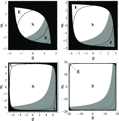
Figure 4: Analysis of the remote entanglement $\varepsilon$ on the correlation plane $(g,g^{\prime})$ for different values of the transmissivity $\tau=0.3$, $0.5$, $0.75$, and $0.9$ (from top left to bottom right). Corresponding values of the thermal noise are determined by the one-mode EB condition $\omega=\omega_{\text{EB}}$. In each inset, the non-black area identifies the set of physical environments, which are divided into separable (S) and entangled (E) environments by the solid lines. The gray region is the “activation area” and identifies those environments for which Charlie is able to distribute entanglement to Alice and Bob ($\varepsilon<1$). Within the activation area, the environments below the dashed curve are those for which the distributed entanglement is also distillable by one-way protocols ($\varepsilon<e^{-1}$). Figure is re-used from Ref. NJP under a CC BY 3.0 licence (http://creativecommons.org/licenses/by/3.0/).

In Fig. 4, the environments identified by the gray activation area allow Charlie to distribute entanglement to Alice and Bob ($\varepsilon<1$), despite it is impossible for him to share entanglement with any of the remote parties. In other words, these environments are two-mode entanglement preserving (EP), despite being one-mode EB. Furthermore, one can identify sufficiently-correlated environments for which the entanglement distributed to the remote parties can also be distilled ($\varepsilon<e^{-1}$).

The most remarkable feature in Fig. 4 is represented by the presence of separable environments in the activation area. In other words, there are separable environments which contain enough correlations to restore the distribution of entanglement to Alice and Bob. Furthermore, for sufficiently high transmissivities and correlations, these environments enable Charlie to distribute distillable entanglement. As we can note from Fig. 4, the weight of separable environments in the activation area increases for increasing transmissivities, with the entangled environments almost disappearing for $\tau=0.9$.

III Entanglement swapping in a correlated Gaussian environment

In this section we consider the indirect distribution of entanglement, i.e., the protocol of entanglement swapping. We start with a brief review of this protocol in the ideal case of no noise. Then, we generalize its theory to the case of correlated-noise Gaussian environments, where we prove how entanglement swapping can be reactivated in the presence of one-mode EB.

III.1 Entanglement swapping in the absence of noise

Consider two remote parties, Alice and Bob, who possess two identical EPR states with CM given in Eq. (11). At Alice’s station, the EPR state describes modes $a$ and $A$, while at Bob’s station it describes modes $b$ and $B$. Alice and Bob keep modes $a$ and $b$, while sending modes $A$ and $B$ to Charlie, where a Bell measurement is performed. This means that the travelling modes $A$ and $B$ are combined in a balanced beam splitter whose output modes “$-$” and “$+$” are homodyned, with mode “$-$” measured in the position quadrature and mode “$+$” in the momentum quadrature. In other words, Charlie measures the two EPR quadratures $\hat{q}_{-}:=(\hat{q}_{A}-\hat{q}_{B})/\sqrt{2}$ and $\hat{p}_{+}:=(\hat{p}_{A}+\hat{p}_{B})/\sqrt{2}$. The Bell measurement provides two classical outcomes, $q_{-}$ and $p_{+}$, which can be compacted into a single complex variable $\gamma:=q_{-}+ip_{+}$. The classical variable $\gamma$ is finally communicated to Alice and Bob, with the result of projecting their remote modes $a$ and $b$ into a conditional state $\rho_{ab|\gamma}$ (see Fig. 5).

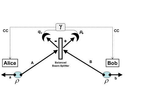
Figure 5: Entanglement swapping in the absence of noise. See text for explanation.

Since the input states are pure Gaussian and the Bell measurement is a Gaussian measurement which projects pure states into pure states, we have that the remote conditional state $\rho_{ab|\gamma}$ turns out to be a pure Gaussian state. This state has a measurement-dependent mean $\mathbf{x}=\mathbf{x}(\gamma)$ which Alice and Bob can always delete by conditional displacements. It is clear that these local unitaries do not alter the amount of entanglement in the state, as long as they are perfectly implemented. The conditional CM $\mathbf{V}_{ab|\gamma}$ can be computed using a simple input-output formula for Gaussian entanglement swapping GaussSWAP . We get

$$\mathbf{V}_{ab|\gamma}=\frac{1}{2\mu}\left(\begin{array}[c]{cc}(\mu^{2}+1)\mathbf{I}&(\mu^{2}-1)\mathbf{Z}\\ (\mu^{2}-1)\mathbf{Z}&(\mu^{2}+1)\mathbf{I}\end{array}\right)~{}.$$ (23)

Its smallest PTS eigenvalue is equal to $\varepsilon=\mu^{-1}$, which means that remote entanglement is always generated for entangled inputs ($\mu>1$). Furthermore, remote entanglement is present in the form of EPR correlations since the two remote EPR quadratures $\hat{q}_{-}^{r}:=(\hat{q}_{a}-\hat{q}_{b})/\sqrt{2}$ and $\hat{p}_{+}^{r}:=(\hat{p}_{a}+\hat{p}_{b})/\sqrt{2}$ have variances

$$V(\hat{q}_{-}^{r})=V(\hat{p}_{+}^{r})=\mu^{-1}~{}.$$ (24)

The simplest description of the entanglement swapping protocol can be given when we consider the limit for $\mu\rightarrow\infty$. In this case the initial states are ideal EPR states with quadratures perfectly correlated, i.e., $\hat{q}_{a}=\hat{q}_{A}$ and $\hat{p}_{a}=-\hat{p}_{A}$ for Alice, and $\hat{q}_{b}=\hat{q}_{B}$ and $\hat{p}_{b}=-\hat{p}_{B}$ for Bob. Then, the overall action of Charlie, i.e., the Bell measurement plus classical communication, corresponds to create a remote state with

$$\hat{q}_{b}=\hat{q}_{a}-\sqrt{2}q_{-},~{}\hat{p}_{b}=-\hat{p}_{a}-\sqrt{2}p_{+}~{}.$$ (25)

The quadratures of the two remote modes are perfectly correlated, up to an erasable displacement. In other words, the ideal EPR correlations have been swapped from the initial states to the final conditional state $\rho_{ab|\gamma}$.

III.2 Entanglement swapping in the presence of correlated-noise

The theory of entanglement swapping can be extended to include the presence of loss and correlated noise. We consider our model of correlated Gaussian environment with transmission $\tau$, thermal noise $\omega$ and correlations $\mathbf{G}$. The modified scenario is depicted in Fig. 6.

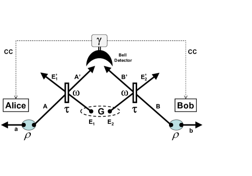
Figure 6: Entanglement swapping in the presence of loss, thermal noise and environmental correlations (correlated Gaussian environment). The Bell detector has been simplified.

III.2.1 Swapping of EPR correlations

For simplicity, we start by studying the evolution of the EPR correlations under ideal input conditions ($\mu\rightarrow+\infty$). After the classical communication of the outcome $\gamma$, the quadratures of the remote modes $a$ and $b$ satisfy the asymptotic relations

$$\hat{q}_{b} =\hat{q}_{a}-\sqrt{\frac{2}{\tau}}\left(q_{-}-\sqrt{1-\tau}\hat{\delta}_{q}\right),$$ (26)

$$\hat{p}_{b} =-\hat{p}_{a}-\sqrt{\frac{2}{\tau}}\left(p_{+}-\sqrt{1-\tau}\hat{\delta}_{p}\right),$$ (27)

where $\hat{\delta}_{q}=(\hat{q}_{E_{1}}-\hat{q}_{E_{2}})/\sqrt{2}$ and $\hat{\delta}_{p}=(\hat{p}_{E_{1}}+\hat{p}_{E_{2}})/\sqrt{2}$ are noise variables introduced by the environment.

Using previous Eqs. (26) and (27), we construct the remote EPR quadratures $\hat{q}_{-}^{r}$ and $\hat{p}_{+}^{r}$, and we compute the EPR variances

$$\boldsymbol{\Lambda}:=\left(\begin{array}[c]{cc}V(\hat{q}_{-}^{r})&\\ &V(\hat{p}_{+}^{r})\end{array}\right)\rightarrow\boldsymbol{\Lambda}_{\infty}=\frac{1-\tau}{\tau}(\omega\mathbf{I}-\mathbf{ZG})~{},$$ (28)

where the limit is taken for $\mu\rightarrow+\infty$. Assuming the EB condition $\omega=\omega_{\text{EB}}$, we finally get

$$\boldsymbol{\Lambda}_{\infty,\text{EB}}=\frac{1}{\tau}\left[(1+\tau)\mathbf{I}-(1-\tau)\mathbf{ZG}\right].$$ (29)

In the case of a memoryless environment ($\mathbf{G=0}$) we see that $\boldsymbol{\Lambda}_{\infty,\text{EB}}=(1+\tau^{-1})\mathbf{I}\geq\mathbf{I}$, which means that the EPR correlations cannot be swapped to the remote systems. However, it is evident from Eq. (29) that there are choices for the correlation block $\mathbf{G}$ such that the EPR condition $\boldsymbol{\Lambda}_{\infty,\text{EB}}<\mathbf{I}$ is satisfied. For instance, this happens when we consider $\mathbf{G=}g\mathbf{Z}$. In this case it is easy to check that $\boldsymbol{\Lambda}_{\infty,\text{EB}}<\mathbf{I}$ is satisfied for $\tau\geq 1/4$ and $g>(1-\tau)^{-1}$. Under these conditions, EPR correlations are successfully swapped to the remote modes. In particular, for $\tau>1/2$ and $g>(1-\tau)^{-1}$ there are separable environments which do the job.

III.2.2 Swapping and distillation of entanglement

Here we discuss in detail how entanglement is distributed by the swapping protocol in the presence of a correlated Gaussian environment. In particular, suppose that Alice and Bob cannot share entanglement with Charlie because the environment is one-mode EB. Then, we aim to address the following questions: (i) Is it still possible for Charlie to distribute entanglement to the remote parties thanks to the environmental correlations? (ii) In particular, is the swapping successful when the environmental correlations are separable? (iii) Finally, are Alice and Bob able to distill the swapped entanglement by means of one-way distillation protocols? Our previous discussion on EPR correlations clearly suggests that these questions have positive answers. Here we explicitly show this is indeed true for quantum entanglement by finding the typical regimes of parameters that the Gaussian environment must satisfy.

In order to study the propagation of entanglement we first need to derive the CM $\mathbf{V}_{ab|\gamma}$ of the conditional remote state $\rho_{ab|\gamma}$. As before, we have two identical EPR states at Alice’s and Bob’s stations with CM $\mathbf{V}(\mu)$ given in Eq. (11). The travelling modes $A$ and $B$ are sent to Charlie through a Gaussian environment with transmissivity $\tau$, thermal noise $\omega$ and correlations $\mathbf{G}$. After the Bell measurement and the classical communication of the result $\gamma$, the conditional remote state at Alice’s and Bob’s stations is Gaussian with CM BellFORMULA

$$\mathbf{V}_{ab|\gamma}=\left(\begin{array}[c]{cc}\mu\mathbf{I}&\\ &\mu\mathbf{I}\end{array}\right)-\frac{(\mu^{2}-1)\tau}{2}\left(\begin{array}[c]{cccc}\frac{1}{\theta}&&-\frac{1}{\theta}&\\ &\frac{1}{\theta^{\prime}}&&\frac{1}{\theta^{\prime}}\\ -\frac{1}{\theta}&&\frac{1}{\theta}&\\ &\frac{1}{\theta^{\prime}}&&\frac{1}{\theta^{\prime}}\end{array}\right)~{},$$ (30)

where

$$\theta=\tau\mu+(1-\tau)(\omega-g),~{}\theta^{\prime}=\tau\mu+(1-\tau)(\omega+g^{\prime})~{}.$$ (31)

From the CM of Eq. (30) we compute the smallest PTS eigenvalue $\varepsilon$ quantifying the remote entanglement at Alice’s and Bob’s stations. For large input entanglement $\mu\gg 1$, we find a closed formula in terms of the environmental parameters, i.e.,

$$\varepsilon=\frac{1-\tau}{\tau}\sqrt{(\omega-g)(\omega+g^{\prime})}:=\varepsilon(\tau,\omega,g,g^{\prime})~{},$$ (32)

which is equal to Eq. (20) up to a factor $\tau^{-1}$. As before, this eigenvalue not only determines the log-negativity but also the coherent information $I(a\rangle b)$ associated with the remote state $\rho_{ab|\gamma}$. In fact, for large $\mu$, one can easily compute the asymptotic expression

$$I(a\rangle b)\rightarrow\log\frac{2}{e}\sqrt{\frac{\det\mathbf{V}_{b|\gamma}}{\det\mathbf{V}_{ab|\gamma}}}=\log\frac{1}{e\varepsilon}~{},$$ (33)

which is identical to the formula of Eq. (21) for the case of direct distribution. Thus, the PTS eigenvalue of Eq. (32) contains all the information about the distribution and distillation of entanglement in the swapping scenario. For $\varepsilon<1$ entanglement is successfully distributed by the swapping protocol (log-negativity $\mathcal{E}>0$). Then, for the stronger condition $\varepsilon<e^{-1}$, the swapped entanglement can also be distilled into $I(a\rangle b)$ entanglement bits per copy by means of one-way protocols.

Now, let us assume the condition of one-mode EB ($\omega=\omega_{\text{EB}}$) so that the bipartite states before measurement $\rho_{aA^{\prime}}$ and $\rho_{B^{\prime}b}$ are separable (see Fig. 6). We investigate the amount of entanglement generated in the remote modes $a$ and $b$ by computing the eigenvalue $\varepsilon(\tau,\omega_{\text{EB}},g,g^{\prime})$. In the standard memoryless case ($\mathbf{G}=\mathbf{0}$) we have $\varepsilon=1+\tau^{-1}$ which means that no entanglement can be swapped, as expected. To study the general case of correlated environment, we consider different numerical values of the transmissivity $\tau$, and we plot the $\varepsilon(\tau,\omega_{\text{EB}},g,g^{\prime})$ on the correlation plane. The results are shown in Fig. 7 and are similar to those achieved in Fig. 4 for direct distribution.

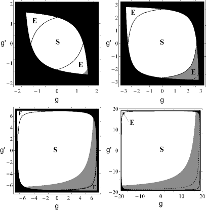
Figure 7: Analysis of the swapped entanglement $\varepsilon$ in the correlation plane $(g,g^{\prime})$ for different values of the transmissivity $\tau=0.3$, $0.5$, $0.75$, and $0.9$ (from top left to bottom right). Corresponding values of the thermal noise are determined by the one-mode EB condition $\omega=\omega_{\text{EB}}$. In each inset, the non-black area identifies the set of physical environments, which are divided into separable (S) and entangled (E) environments. The gray region identifies the activation area, i.e., those environments whose correlations are strong enough to generate remote entanglement ($\varepsilon<1$). Within the gray activation area, the environments that lie below the dashed curve are those able to generate distillable entanglement ($\varepsilon<e^{-1}$).

In each panel of Fig. 7, the physical values for the correlation parameters $(g,g^{\prime})$ are individuated by the non-black area. Remote entanglement is distributed ($\varepsilon<1$) for values of the correlation parameters belonging to the gray activation area. For $\tau\leq 1/2$ (top two panels), we see that the activation area is confined within the region of entangled environments. The property that entangled environments are necessary for the reactivation of entanglement swapping at any $\tau\leq 1/2$ is easy to prove. In fact, suppose that $\varepsilon<1$ holds. By using its formula in Eq. (32) and the bona-fide conditions on the correlation parameters given in Eq. (8), we can write $\varepsilon^{2}<1$ as

$$\omega^{2}-gg^{\prime}+\omega(g^{\prime}-g)<\left(\frac{\tau}{1-\tau}\right)^{2}~{}.$$ (34)

Now, for $\tau\leq 1/2$, we have $\tau^{2}(1-\tau)^{-2}\leq 1$ and using this inequality in Eq. (34), we derive

$$\omega^{2}-gg^{\prime}-1<\omega(g-g^{\prime})\leq\omega|g-g^{\prime}|~{},$$ (35)

which is the entanglement condition for the environment [i.e., the violation of Eq. (10)].

It is clear that the most interesting result holds for transmissivities $\tau>1/2$. In this regime, in fact, the distribution of remote entanglement can be activated by separable environments. As explicitly shown for $\tau=0.75$ and $0.9$, the activation area progressively invades the region of separable environments. In other words, separable correlations become more and more important for increasing transmissivities. Furthermore, for $\tau\gtrsim 0.75$, separable environments are even able to activate the distribution of distillable entanglement ($\varepsilon<e^{-1}$). By comparing Fig. 4 and Fig. 7, we see how entanglement is more easily generated and distilled by the direct protocol. This is a consequence of the extra factor $\tau^{-1}$ in Eq. (32), whose influence becomes less important only at high transmissivities ($\tau\simeq 1$).

IV Conclusion

In conclusion, we have investigated the distribution of entanglement in the presence of correlated-noise Gaussian environments, proving how the injection of separable correlations can recover from entanglement breaking. In order to derive simple analytical results we have considered here only the case of large entanglement for the input states. We have analyzed scenarios of direct distribution and indirect distribution, i.e., entanglement swapping. Surprisingly, the injection of the weaker separable correlations is sufficient to restore the entanglement distribution, as we have shown for wide regimes of parameters. Furthermore, the generated entanglement can be sufficient to be distilled by means of one-way protocols. The fact that separability can be exploited to recover from entanglement breaking is clearly a paradoxical behavior which poses fundamental questions on the intimate relations between local and nonlocal correlations.

References

- (1) Nielsen, M. A. and Chuang, I. L., [Quantum Computation and Quantum Information], Cambridge University Press, Cambridge, (2000).
- (2) Wilde, M. M., [Quantum Information Theory], Cambridge University Press, Cambridge (2013).
- (3) Horodecki, M., Shor, P. W. and Ruskai, M. B., “General Entanglement Breaking Channels,” Rev. Math. Phys 15, 629-641 (2003).
- (4) Holevo, A. S., “Entanglement-breaking channels in infinite dimensions,” Problems of Information Transmission 44, 3-18 (2008).
- (5) Weedbrook, C., Pirandola, S., Garcia-Patron, R., Cerf, N. J., Ralph, T. C., Shapiro, J. H. and Lloyd, S., “Gaussian Quantum Information,” Rev. Mod. Phys. 84, 621 (2012).
- (6) Braunstein, S. L. and Pati, A. K., [Quantum Information Theory with Continuous Variables], Kluwer Academic, Dordrecht (2003).
- (7) Braunstein, S. L. and van Loock, P., “Quantum information with continuous variables,” Rev. Mod. Phys. 77, 513 (2005).
- (8) Pirandola, S., “Entanglement Reactivation in Separable Environments,” New J. Phys. 15, 113046 (2013). Doi:10.1088/1367-2630/15/11/113046.
- (9) Werner, R., “Quantum states with Einstein-Podolsky-Rosen correlations admitting a hidden-variable model,” Phys. Rev. A 40, 4277 (1989).
- (10) Horodecki, M. and Horodecki, P., “Reduction criterion of separability and limits for a class of distillation protocols,” Phys. Rev. A 59, 4206–4216 (1999).
- (11) Einstein, A., Podolsky, B. and Rosen, N., “Can Quantum-Mechanical Description of Physical Reality Be Considered Complete?,” Phys. Rev. 47, 777 (1935).
- (12) Pirandola, S., Serafini A. and Lloyd, S., “Correlation matrices of two-mode bosonic systems,” Phys. Rev. A 79, 052327 (2009).
- (13) Eisert, J., [Entanglement in quantum information theory], PhD thesis, Potsdam (2001).
- (14) Vidal, G. and Werner, R. F., “Computable measure of entanglement,” Phys. Rev. A 65, 032314 (2002).
- (15) Plenio, M. B., “Logarithmic Negativity: A Full Entanglement Monotone That is not Convex,” Phys. Rev. Lett. 95, 090503 (2005).
- (16) Schumacher, B. and Nielsen, M. A., “Quantum data processing and error correction,” Phys. Rev. A 54, 2629 (1996).
- (17) Lloyd, S., “Capacity of the noisy quantum channel,” Phys. Rev. A 55, 1613 (1997).
- (18) Pirandola, S., Vitali, D., Tombesi P. and Lloyd, S., “Macroscopic Entanglement by Entanglement Swapping,” Phys. Rev. Lett. 97, 150403 (2006).
- (19) Spedalieri, G., Ottaviani, C. and Pirandola, S., “Covariance matrices under Bell-like detections,” Open Syst. Inf. Dyn. 20, 1350011 (2013).