Obstacle avoiding patterns and
cohesiveness of fish school

Abstract

This paper is devoted to studying obstacle avoiding patterns and cohesiveness of fish school. First, we introduce a model of stochastic differential equations (SDEs) for describing the process of fish school’s obstacle avoidance. Second, on the basis of the model we find obstacle avoiding patterns. Our observations show that there are clear four obstacle avoiding patterns, namely, Rebound, Pullback, Pass and Reunion, and Separation. Furthermore, the emerging patterns change when parameters change. Finally, we present a scientific definition for fish school’s cohesiveness that will be an internal property characterizing the strength of fish schooling. There are then evidences that the school cohesiveness can be measured through obstacle avoiding patterns.

1 Introduction

Fish schooling, one of animal swarming, is a commonly observed phenomenon that is coherently performed by integration of interactions among constituent fish. This remarkable phenomenon has already attracted interests of researchers from diverse fields including biology, physics, mathematics, computer engineering (see [1, 3, 4, 11, 14, 17, 21, 22, 23, 25, 26]).

Let us recall here some researches in the literature therein. In 2001, Camazine et al. [4, Chapter 11] presented an idea on the basis of experimental results (Aoki [1], Huth-Wissel [14], and Warburton-Lazarus [28]) that individual fish may act following the behavioral rules:

1. The school has no leaders and each fish follows the same behavioral rules.

2. To decide where to move, each fish uses some form of weighted average of the position and orientation of its nearest neighbors.

3. There is a degree of uncertainty in the individual’s behavior that reflects both the imperfect information-gathering ability of a fish and the imperfect execution of the fish’s actions.

Their insight is that these local rules can altogether create the coherent behavior of fish school.

Vicsek et al. [27] modeled the movement as self-driven particles obeying some difference equations. They assumed that each individual is driven with a sum of an absolute velocity and an averaged velocity of nearby particles together with some random perturbations. Oboshi et al. [20] also modeled schooling by some difference equations setting a rule that each fish choose one way of action among four possibilities according to a distance to the closest mate. Meanwhile, Olfati-Saber [21] and D’Orsogna et al. [7] independently presented differential equation models, but deterministic ones, utilizing the generalized Morse function and attractive/repulsive potential functions, respectively. In [11], Gunji et al. considered dual interaction which produces territorial and schooling behavior. In [23], Reynolds introduced some simple behavioral rules of animals, which are similar to (a), (b), (c) but deterministic ones, and are schematic rather than physical.

A stochastic differential equation (SDE) model describing the process of schooling was presented in [26], where we used the behavioral rules (a), (b), and (c) above. We then utilized the model for developing quantitative arguments on fish schooling in [17].

In the real world, the environment surrounding fish school often includes other components such as obstacles, food resources, predators, etc. In those situations, fish exhibit more complex, parallel movements such as obstacle avoidance, food finding, escaping from predator. It is evident that when a school of fish is tackled by obstacles or is hunted by predators, fish individually react quickly for avoiding obstacles or predators.

Olfati-Saber and Murray [22] developed the method of Reynolds [23] by introducing a dynamic graph of agents in the presence of multiple obstacles. The agents are split into several groups while approaching the obstacles. After passing all obstacles, they rejoin into a single group. Chang et al. [6] introduced techniques of using gyroscopic forces for multi-agent systems by which the agents perform collision avoidance toward obstacles. A similar result has been shown (i.e., agents are separated into some clusters and then rejoin into a single flock). In the meantime, Hettiarachchi and Spears [12] used virtual physical forces in composing a swarm system of robots moving toward a goal through obstacle fields. Robots may collide with obstacles but then they can still move toward the goal.

In the meantime, a concept concerning animal swarming or grouping, namely cohesiveness has already been introduced since 1930s. The study during long years seems to show that it is not an easy problem to define a concept of the cohesiveness precisely and consistently. It has been conceptualized in various ways, but each was based on intuitive assumptions and interpretations.

For instance, Moreno and Jennings [18] defined cohesiveness as the forces holding the individuals within the group to which they belong. French [9] noted that the group exists as a balance between cohesion and disruptive forces. Not until 1950 was a systematic theory of group cohesiveness constructed by Festinger et al. [8]. Their definition of cohesiveness is “We shall call the total field of forces which act on members to remain in the group the “cohesiveness” of that group”. Gross and Martin [10] claimed that this definition is inadequate, and they proposed an alternative definition as the resistance of group to disruptive forces. Contemporary works almost characterize group cohesion in the same way (see [13]). Carron [5] defined cohesiveness to be the adhesive property of group. Schachter et al. [24] found that interpersonal attraction is the cement binding group members together. For the general relationship between cohesiveness and group performance, we refer the reader to [2, 16, 19].

We can however find a point of view which is common in those definitions. That is the bond linking group members to others and to the group as a whole. We believe that this common point of view may be a key feature for all intercommunicated multi-agent systems.

The objective of the present paper is two-folds: namely, studying the fish schooling from a viewpoint of pattern formation of biological systems and introducing a scientific definition of the school cohesiveness.

For the first objective, obstacle avoiding patterns of fish school are studied by newly introducing a behavioral rule for avoidance and adding its effect to our model in [26]. It is then observed that there are at least four obstacle avoiding patterns of school, i.e., Rebound, Pullback, Pass and Reunion, and Separation which are performed just by tuning modeling parameters.

For the second objective, we consider school cohesiveness as its ability to form and maintain the school structure against the white noises affecting the school. It is therefore defined as an internal nature of the school, independent of external effects. We then show how internal parameters contribute to the school’s cohesiveness. Furthermore, our results suggest a very interesting correlation between the degree of cohesiveness and the four avoidance patterns.

The outline of this paper is as follows. Section 2 gives model description. We first recall the SDE model for fish schooling introduced in [26], then newly inoculate a mechanism for obstacle avoiding into it. Section 3 presents four obstacle avoiding patterns. We thereafter investigate how these patterns change as the modeling parameters are tuned. Section 4 explores fish school cohesiveness. A scientific definition and measurement of cohesiveness are introduced. The relationship between avoidance patterns and school cohesiveness is then investigated. The paper concludes with some discussions of Section 5.

2 Model description

In [26], we introduced a SDE model of the form

$$\begin{cases}d{\mathbf{x}}_{i}(t)&={\mathbf{v}}_{i}dt+\sigma_{i}dw_{i}(t),\\ d{\mathbf{v}}_{i}(t)&=\Big{\{}-\alpha\sum\limits_{j=1,j\neq i}^{N}\left(\dfrac{r^{p}}{\|{\mathbf{x}}_{i}-{\mathbf{x}}_{j}\|^{p}}-\dfrac{r^{q}}{\|{\mathbf{x}}_{i}-{\mathbf{x}}_{j}\|^{q}}\right)({\mathbf{x}}_{i}-{\mathbf{x}}_{j})\\ &\qquad-\beta\sum\limits_{j=1,j\neq i}^{N}\left(\dfrac{r^{p}}{\|{\mathbf{x}}_{i}-{\mathbf{x}}_{j}\|^{p}}+\dfrac{r^{q}}{\|{\mathbf{x}}_{i}-{\mathbf{x}}_{j}\|^{q}}\right)({\mathbf{v}}_{i}-{\mathbf{v}}_{j})\\ &\qquad+F_{i}({\mathbf{x}}_{i},{\mathbf{v}}_{i})\Big{\}}dt,\hfill i=1,2,\ldots,N,\end{cases}$$ (1)

for an $N$-fish system moving in the space $\mathbb{R}^{d}$ ($d=2,3$). Here, ${\mathbf{x}}_{i}(t)$ and ${\mathbf{v}}_{i}(t)$ denote position and velocity of the $i$-th fish at time $t$, respectively. And $\|\cdot\|$ denote the Euclidean norm of a vector, hence $\|{\mathbf{x}}_{i}-{\mathbf{x}}_{j}\|$ represents the distance between the $i$-th and the $j$-th fish.

We regarded each fish as a moving particle in $\mathbb{R}^{d}$. The first equation is a stochastic equation for the unknown ${\mathbf{x}}_{i}(t)$, where $\sigma_{i}dw_{i}$ denotes noise resulting from the imperfectness of information-gathering and action of the $i$-th fish. In fact, $w_{i}(\cdot)(i=1,2,\dots,N)$ are independent $d$-dimensional Brownian motions on some probability space.

The second equation is a deterministic equation for ${\mathbf{v}}_{i}(t)$, where $1<p<q<\infty$ are fixed exponents; $\alpha$ and $\beta$ are positive coefficients of attraction and velocity matching among fish, respectively. And $r>0$ is a fixed number. If $\|{\mathbf{x}}_{i}-{\mathbf{x}}_{j}\|>r$ then the $i$-th fish moves toward the $j$-th. To the contrary, if $\|{\mathbf{x}}_{i}-{\mathbf{x}}_{j}\|<r$ then the $i$-th fish acts in order to avoid collision with the $j$-th, $r$ being thereby a critical distance (for details, see [26]).

Velocity matching of the $i$-th fish to the $j$-th also has a similar weight depending on the distance $\|{\mathbf{x}}_{i}-{\mathbf{x}}_{j}\|$. Degree of matching is higher when $\|{\mathbf{x}}_{i}-{\mathbf{x}}_{j}\|<r$ for urgent reaction to avoid collision. When $p$ is large, the attraction range is short. Meanwhile, when $p$ is small, fish have ability to attract each other against a long distance. The exponent $p$ thereby relates to a degree of how far the attraction reaches. Finally, the function $F_{i}({\mathbf{x}}_{i},{\mathbf{v}}_{i})$ stands for an external force function acting on the $i$-th fish.

The system (1) was studied analytically and numerically in the subsequent paper [17] of [26]. Quantitative arguments on fish schooling were also developed. Main advantages of using SDE models like (1) over others may be the convenience of mathematical technique. One can utilize the well developed theory of SDEs including numerical methods (see [15]). Its flexibility may be another advantage. As seen below, it is very easy to modify the model in the existence of an obstacle simply by introducing a suitable external force functions $F_{i}(\mathbf{x}_{i},\,\mathbf{v}_{i})$ in (1).

We now want to study (1) from the viewpoint of obstacle avoiding. For this purpose, let us put a global obstacle with central point ${\mathbf{x}}_{C}$ and radius $\rho>0$ in $\mathbb{R}^{d}$ and assume that fish move in the domain $\Omega=\{{\mathbf{x}}\in\mathbb{R}^{d}:\|{\mathbf{x}}-{\mathbf{x}}_{C}\|>\rho\}$. The surface of the obstacle is denoted by $S=\{\mathbf{x}\in\mathbb{R}^{d}:\|{\mathbf{x}}-{\mathbf{x}}_{C}\|=\rho\}$. In addition to the rules (a)-(c) in Introduction, we introduce a behavioral rule in order to avoid collision with the obstacle:

• Each fish executes an action for avoiding the obstacle according to a reflection law of velocity with distance depending weight.

On the basis of this rule, we are able to formulate the external force function $F_{i}(x_{i},v_{i})$ which influences the motion of the $i$-th individual. For a given $({\mathbf{x}}_{i},{\mathbf{v}}_{i})$, where $\|{\mathbf{x}}_{i}-{\mathbf{x}}_{C}\|>\rho$, let $l_{i}$ be a ray with origin ${\mathbf{x}}_{i}$ and direction ${\mathbf{v}}_{i}$, i.e.,

$$l_{i}=\{{\mathbf{x}}\in\mathbb{R}^{d}:{\mathbf{x}}={\mathbf{x}}_{i}+s{\mathbf{v}}_{i},\quad 0\leqslant s<\infty\}.$$

When $l_{i}$ intersects $S$, we define ${\rm Rf}({\mathbf{x}}_{i},{\mathbf{v}}_{i})$ as the reflection vector ${\mathbf{u}}_{i}$ of ${\mathbf{v}}_{i}$ at ${\mathbf{y}}_{i}$ with respect to the tangential plane of $S$ at ${\mathbf{y}}_{i}$, where ${\mathbf{y}}_{i}$ is the first intersection of $l_{i}$ to $S$. In fact, ${\mathbf{u}}_{i}$ is a vector whose opposite equals to the symmetric vector of ${\mathbf{v}}_{i}$ over the line connecting ${\mathbf{y}}_{i}$ and ${\mathbf{x}}_{C}$ on the plane generated by ${\mathbf{v}}_{i}$ and ${\mathbf{x}}_{C}$. When $l_{i}$ does not intersect $S$ (including the special case when ${\mathbf{v}}_{i}={\mathbf{0}}$), we put ${\rm Rf}({\mathbf{x}}_{i},{\mathbf{v}}_{i})={\mathbf{v}}_{i}$. Fig. 1 illustrates $({\mathbf{x}}_{i},{\mathbf{v}}_{i})$ and ${\rm Rf}({\mathbf{x}}_{i},{\mathbf{v}}_{i})$ in two-dimensional space.

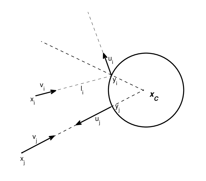
Figure 1: Reflection vector ${\rm Rf}(\mathbb{x}_{i},\mathbb{v}_{i})=\mathbb{u}_{i}$

Analogously to the velocity matching, we formulate

$$F_{i}({\mathbf{x}}_{i},{\mathbf{v}}_{i})=-\gamma\left(\frac{R^{P}}{\|{\mathbf{x}}_{i}-{\mathbf{y}}_{i}\|^{P}}+\frac{R^{Q}}{\|{\mathbf{x}}_{i}-{\mathbf{y}}_{i}\|^{Q}}\right)[{\mathbf{v}}_{i}-{\rm Rf}({\mathbf{x}}_{i},{\mathbf{v}}_{i})],$$ (2)

where $1<P<Q<\infty$ are exponents, $R$ is a fixed distance, and $\gamma>0$ is a constant.

If $\|{\mathbf{x}}_{i}-{\mathbf{y}}_{i}\|<R$, then the $i$-th fish promptly reacts for matching its velocity to the reflection vector ${\rm Rf}({\mathbf{x}}_{i},{\mathbf{v}}_{i})$ to avoid collision with the obstacle. Meanwhile, if $\|{\mathbf{x}}_{i}-{\mathbf{y}}_{i}\|>R,$ then the reaction to avoid the obstacle is less strong. If the ray $l_{i}$ does not meet $S$, the individual takes no reaction with the obstacle.

The model for fish schooling in obstacle domain is therefore of the form (1) with the external forces $F_{i}({\mathbf{x}}_{i},{\mathbf{v}}_{i})$ $(i=1,2,\ldots,N)$ given by (2).

3 Obstacle avoiding patterns

In this section, we observe four avoidance patterns of fish school based on our model (1), where the external force functions $F_{i}({\mathbf{x}}_{i},{\mathbf{v}}_{i})\,(i=1,\dots,N)$ are defined by (2). The effect of control parameters to these patterns is also investigated.

3.1 $\varepsilon$-Graph and $\varepsilon,\theta$-Schooling

Let us review notions of $\varepsilon$-Graph and $\varepsilon,\theta$-Schooling that were introduced in the paper [17].

Definition 3.1 ($\varepsilon$-Graph)

Let ${\mathbf{x}}_{i},{\mathbf{v}}_{i}$ $(i=1,2,\ldots,N)$ denote a solution to SDEs (1). Let $\varepsilon>0$ be a fixed length. Regard the positions ${\mathbf{x}}_{i}(t)$ of fish at each time $t$ as the vertices of a graph. Two vertices ${\mathbf{x}}_{i}(t)$ and ${\mathbf{x}}_{j}(t)$ are said to be connected by an edge of graph if and only if $\|{\mathbf{x}}_{i}(t)-{\mathbf{x}}_{j}(t)\|\leqslant\varepsilon$. Such a graph is called the $\varepsilon$-graph of group at time $t$ and is denoted by ${\rm G}_{\varepsilon}(t)$.

Denote by $n_{\varepsilon}(t)$ the number of connected components of ${\rm G}_{\varepsilon}(t)$. When $n_{\varepsilon}(t)=1$, the individuals form a single group. Meanwhile, when $n_{\varepsilon}(t)\geqslant 2$, they form $n_{\varepsilon}(t)$ sub-groups.

Denote by $\sigma{\rm V}(t)$ the variation of velocities:

$$\sigma{\rm V}(t)=\sqrt{\frac{1}{N}\sum\limits_{i=1}^{N}\|{\mathbf{v}}_{i}(t)-\bar{\mathbf{v}}(t)\|^{2}},\hskip 56.9055pt0<t<\infty,$$

where $\bar{\mathbf{v}}(t)=\frac{1}{N}\sum\limits_{i=1}^{N}{\mathbf{v}}_{i}(t)$ is the average of all velocities of fish at time $t$.

Definition 3.2 ($\varepsilon,\theta$-Schooling)

Let $\varepsilon>0$ and $\theta>0$ be given. If a solution $({\mathbf{x}}_{i},{\mathbf{v}}_{i})$ $(i=1,2,\ldots,N)$ to (1) satisfies $n_{\varepsilon}(t)=1$ and $\sigma{\rm V}(t)\leqslant\theta$ for all sufficiently large $t$, say all $t\geqslant T$ with some fixed time $T>0$, then the state of fish is said to be in $\varepsilon,\theta$-schooling.

When the distance $\varepsilon>0$ and the tolerance $\theta>0$ are specified, we simply say “in schooling” instead of “in $\varepsilon,\theta$-schooling”.

3.2 Obstacle avoiding patterns

Set parameters as $d=2$, $N=20$, $\alpha=\beta=\gamma=1$. The exponent $p$ is tuned from 2 to 4 keeping always the relation $q=p+1$ and $\sigma_{i}=0$ for all $i$. The critical distance $r$ is set by $r=0.5$, and the radius of the obstacle is $\rho=1.2$. In addition, $\varepsilon=0.5$ and $\theta=10^{-6}$.

By performing preliminary computations, we first set a stationary state which is in $\varepsilon,\theta$-schooling. This state is set as the initial position of our computations. The distance from the center of the school to the center of the obstacle is 3.5, and the line connecting these two centers coincides with the horizontal axis. The initial velocities are ${\mathbf{v}}_{i}(0)=(1.75,\,0)$ for every $i$. Parameters for obstacle avoidance are set as $P=p$, $Q=q$, $R=r$. The school is thereby oriented toward the obstacle and will strike on it after a while.

Fig. 2 shows the numerical results for $p=2,\,3,\,3.62,\,4$. Four different kinds of avoiding patterns are found. We will call them, Rebound, Pullback, Pass and Reunion, and Separation, respectively.

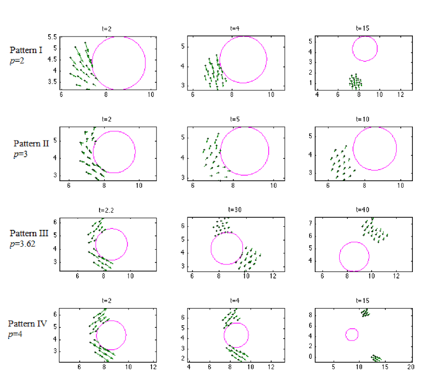
Figure 2: Obstacle avoiding patterns in two-dimensional space: Rebound, Pullback, Pass and Reunion, and Separation

Let us describe these four patterns of fish schooling.

Pattern I (Rebound): The fish keep schooling throughout the obstacle avoiding process and the school rebounds off the obstacle. In order to keep being in schooling, they change their directions after the school touch the obstacle.

Pattern II (Pullback): The individuals are once separated while approaching the obstacle and stay around the surface of obstacle for a while. They then pull back off the obstacle to reform a school structure.

Pattern III (Pass and Reunion): The fish pass the obstacle by spliting to move along the obstacle surface. After passing it they reunite into a single school.

Pattern IV (Separation): It is similar to Pattern III. But, after passing the obstacle, the subgroups have their own direction.

Similar results are observed in the three-dimensional case, i.e., $d=3$ too. Numerical solutions to (1) show that there are similarly four avoidance patterns (I)-(IV).

Fig. 3 represents four behavioral patterns of fish school while avoiding a static sphere obstacle in three-dimensional space. Four rows in this figure illustrate the time evolution of school starting from different initial speeds $v_{0}=0.3,\,2.5,\,6,13.5$, respectively, while the other parameters are kept being constant in such a way that $p=2$, $\alpha=\beta=\gamma=2$, $r=1$. Initial positions of fish are set in $\varepsilon,\theta$-schooling, where $\varepsilon=1$ and $\theta=10^{-6}$.

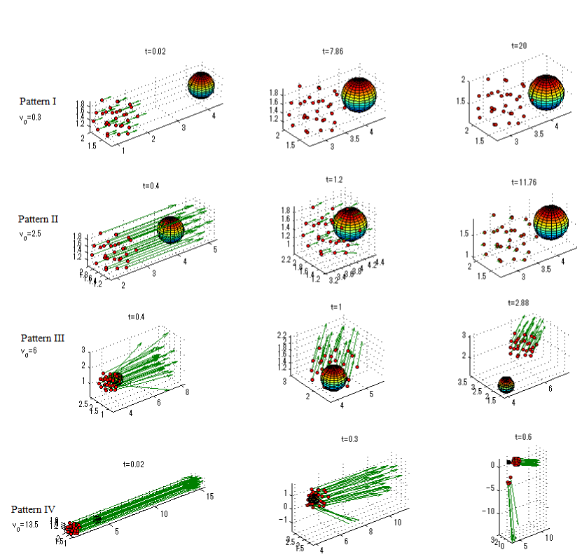
Figure 3: Obstacle avoiding patterns in three-dimensional space: Rebound, Pullback, Pass and Reunion, and Separation

3.3 Exponents $p,q$ and obstacle avoiding patterns

Set the parameters: $d=2$, $N=20$, $\alpha=\beta=\gamma=1$, $r=0.5$, $\rho=1.2$, $\varepsilon=0.5$ and $\theta=10^{-6}$ as Subsection 3.2. The initial data (velocity and position) are also the same.

The exponent $p$ is however finely tuned from 1.001 to 8 with increment $\Delta p=0.001$ and the relation $q=p+1$ is always kept. In addition, $P=p$, $Q=q$, $R=r$.

Our numerical results are presented in Table 1. This table highlights that there are critical values of $p$ at which the type of avoidance patterns changes from I to II, from II to III, and from III to IV, respectively.

Table 1: Exponent $p$ and patterns

$p$	[1.001,  2.100]	[2.101,  3.371]	[3.372, 3.497]	[3.498, 8.000]
Pattern	I	II	III	IV

3.4 Speeds of school and obstacle avoiding patterns

We set a fish group being in schooling. We investigate relations between the speed of school $\|\bar{v}\|$ and the type of performed pattern.

Table 2 shows our numerical results in two-dimensional case. Here $N=20$, $\alpha=\beta=\gamma=1$, $p=2$, $r=0.5$, and the distance from the center of fish in schooling to the center of the obstacle is 3.5. The increment $\Delta\|v_{0}\|$ is also 0.001.

Table 2: Speeds of school and patterns

$\|v_{0}\|$	[0.001,  1.199]	[1.200,  2.589]	[2.590, 4.866]	[4.867, 20]
Pattern	I	II	III	IV

Of course, if the initial speed is too large, then collision may happen because the large velocity makes fish have no enough time to adjust to avoid collision with other fish or with the obstacle. We do not consider this case. It is, however, interesting to know that solutions to (1), where $F_{i}(i=1,2,\dots,N)$ are given by (2), can blow up in a finite time.

3.5 Critical distance $r$ and obstacle avoiding patterns

Let tune the critical distance $r$ from 0.2 to 2.8 with increment $\Delta r=0.1$. Other parameters are $d=2$, $N=20$, $\alpha=\beta=\gamma=1$, $\rho=1.2$, $P=p=3$, $Q=q=4$, $\varepsilon=R=r$, $\theta=10^{-6}$.

In order to set the initial positions, we perform preliminary computations for each $r$ in the free space $\mathbb{R}^{2}$, where $F_{i}=-5{\mathbf{v}}_{i}$. These computations provide stationary states in $\varepsilon,\theta$-schooling for each $r$.

As pointed out by [17], the geometrical diameter $\delta$

$$\delta=\max_{1\leqslant i\leqslant N}\|{\mathbf{x}}_{i}-\bar{\mathbf{x}}\|\hskip 28.45274pt\text{with }\bar{\mathbf{x}}=(\sum_{i=1}^{N}{\mathbf{x}}_{i})/N$$

of $\varepsilon,\theta$-schooling depends on $r$. It is thus natural to choose different radius of obstacle depending on $r$. In the present computations, the radius of obstacle is set as $\rho=2\delta(r)/3$, where $\delta(r)$ is the school diameter corresponding to $r$. The distance from the center of school to the center of obstacle is 8, and the line connecting these two centers coincides with the horizontal axis. The initial velocities are ${\mathbf{v}}_{i}(0)=(4,0)$ for all $i$.

Our numerical results given in Table 3 show that as $r$ increases, the type of patterns changes from IV to III, from III to II, and from II to I.

Table 3: Critical distance and patterns

$r$	[0.2,  0.3]	[0.4,  0.5]	[0.6, 2.0]	[2.1, 2.8]
Pattern	IV	III	II	I

4 School cohesiveness

In this section, we want to introduce a scientific definition of cohesiveness possessed by fish school as a nature of school. We then investigate the relationships between school cohesiveness and obstacle avoiding patterns. These relationships suggest that avoidance patterns can be used to visualize the school cohesiveness.

4.1 Definition and measurement of school cohesiveness

Let us first introduce a scientific definition of cohesiveness for the system (1) of SDEs in free space.

Definition 4.1

School cohesiveness is the ability of group of fish to form and maintain the $\varepsilon,\theta$-schooling structure against the noise imposed on the school. In other words, how far the group can keep on $\varepsilon,\theta$-schooling as the magnitudes of the noises increase.

This definition is given in a quantitative form. When $\varepsilon$ and $\theta$ are specified, it is possible to quantitatively measure the cohesiveness of a group.

Let us next give some examples of measuring cohesiveness of fish school by numerical methods.

Consider a group of 50 fish moving in $\mathbb{R}^{2}$. The parameters are set as $p=4$, $q=5$, $\alpha=4$, $\beta=1$. The external force functions are taken as $F_{i}=-{\mathbf{v}}_{i}$ for $i=1,2,\ldots,N$. Initial positions ${\mathbf{x}}_{i}(0)$ are randomly located in a suitably small domain with null initial velocities ${\mathbf{v}}_{i}(0)={\mathbf{0}}$. The magnitude $\sigma_{i}\equiv\sigma$ is a control parameter of simulation.

We pick out 20 different trajectories of the Wiener process. For each value $\sigma$, numerical computations for the solution ${\mathbf{x}}_{i}(t)$ and ${\mathbf{v}}_{i}(t)$ are performed in 20 trials corresponding to these trajectories.

Set $\varepsilon=r=0.5$ and $\theta=0.05$. It is examined whether or not the states $({\mathbf{x}}_{i}(t),{\mathbf{v}}_{i}(t))(i=1,2,\dots,N)$ are in $\varepsilon,\theta$-schooling by fixing $T=30$. In other words, it is checked that whether or not $n_{\varepsilon}(t)=1$ and $\sigma V(t)\leq\theta$ for every $t\geq 30$.

Starting with sufficiently small $\sigma$, $\sigma$ is then increased with increment step 0.001. When the $\varepsilon,\theta$-schooling structure is broken down at least for one sample trajectory of the Wiener process, the fish are considered to have lost ability of schooling. The critical value of $\sigma$ which is the largest value of $\sigma$ such that the group is still in $\varepsilon,\theta$-schooling can then be found.

Fig. 4 shows that when $\sigma=0.02$, the group builds up the $\varepsilon,\theta$-schooling structure. Here, the sub-figure on the left shows the $\varepsilon$-graph of the group at time $t=30$, the positions ${\mathbf{x}}_{i}(t)$ being drawn by dots, and the edges of graph by lines. The right hand side sub-figure illustrates the variance of velocity as a function of $t$, where the horizontal line represents the level $\theta=0.05$.

The group loses schooling ability when $\sigma=0.06$. In fact, Fig. 5 demonstrates that $n_{\varepsilon}(t)=2$ for $t=30$. Schooling ability of the group is also lost when $\sigma=0.069$. Fig. 6 highlights that $\sigma{\rm VS}(t)>\theta$ for $t=30$.

By these methods, we can finally compute the critical value $\bar{\sigma}=0.051$. The group is in $\varepsilon,\theta$-schooling whenever $\sigma\leq\bar{\sigma}$, whereas it loses schooling ability whenever $\sigma>\bar{\sigma}$.

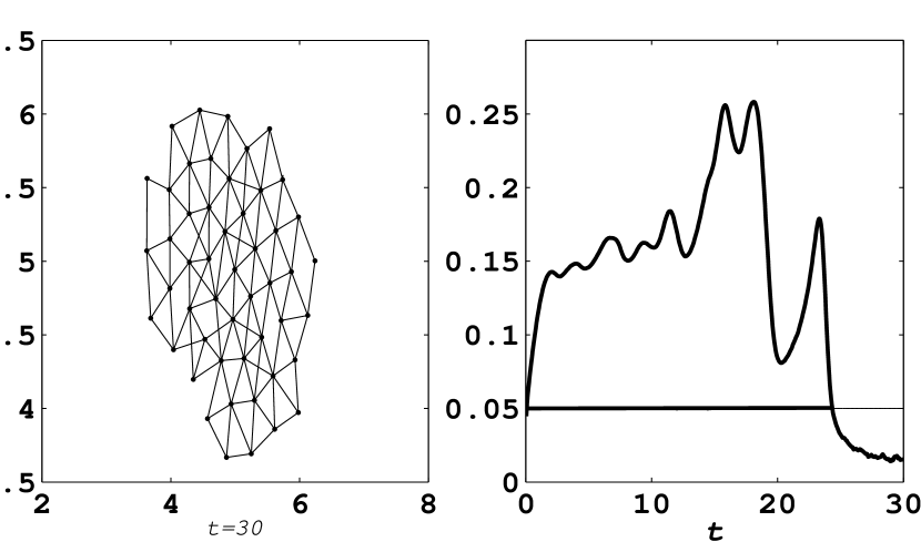
Figure 4: $\varepsilon$-graph and $\sigma{\rm VS}(t)$ for $\sigma=0.02$

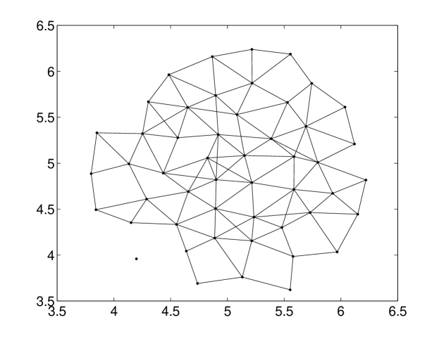
Figure 5: $\varepsilon$-graph for $\sigma=0.06$

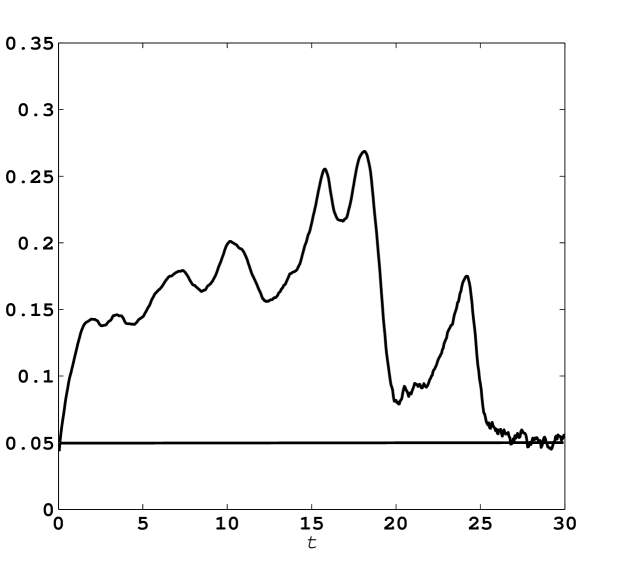
Figure 6: $\sigma{\rm VS}(t)$ for $\sigma=0.069$

4.2 Relations between exponents $p,q$ and school cohesiveness

Let tune $p$ as $p=4,\,3.62,\,3,\,2$, keeping the relation $q=p+1$ and other parameters as before. Our computations show that the numerical critical value of $\sigma$, namely the cohesiveness, changes as $\bar{\sigma}=0.051,\,0.055,\,0.056,\,0.063,$ respectively.

The exponent $p$, as explained in Section 2, shows a degree of range how far the attraction is effective. It is therefore very natural that as $p$ decreases, the attraction range extends and enhances the cohesiveness of group.

4.3 Relations between critical distance and school cohesiveness

Let us tune $r$ from 0.5, 0.6 and 0.7 by taking $\varepsilon=r$, $p=4$, $q=5$, $\theta=0.05$, $T=30$. The corresponding cohesiveness is found as $\bar{\sigma}=0.051,0.053,0.054,$ respectively. This means that cohesiveness is enhanced as the critical distance increases.

4.4 Relationship between school cohesiveness and obstacle avoiding patterns

In Subsections 3.2 and 3.3, we already show that suitable tuning of the exponents $p$ and $q=p+1$ provides different obstacle avoiding patterns. It is possible to interpret this fact as follows.

Note that $p$ is concerned with the range of attraction among fish. If $p$ is small, then the attractive force reaches a wide range beyond the critical distance $r$. In contrast, if $p$ is large, then the attraction is only available in a neighborhood of the disk of radius $r$. In Subsection 4.2, we verify that when other parameters are fixed, the cohesiveness of school increases as $p$ decreases.

In the numerical examples in Subsection 3.2, when $p=2$, the school has very strong cohesiveness and rebounds off the obstacle. When $p=3$, the school still has strong cohesiveness and can keep schooling. But the fish are spread on the surface. When $p=3.62$, the school cohesiveness becomes smaller. The fish can no longer keep being in schooling but it is strong enough to reunite the members into a school. When $p=4$, the school cannot keep being in schooling and is separated into two clusters after passing the obstacle.

If these interpretations are reasonable, then the four obstacle avoiding patterns can be used to measure the cohesiveness of school approximately. For example, the cohesiveness can be easily categorized into four classes.

5 Conclusions

Obstacle avoiding patterns and cohesiveness of fish school have been studied. In fact, our mathematical model for fish schooling in the space with obstacles provided four clear avoidance patterns: Rebound, Pullback, Pass and Reunion, and Separation. The shift from one pattern to another due to the change of parameters has also been investigated.

Furthermore, our definition for school cohesiveness suggested that the cohesiveness can roughly be measured by using the four types of patterns. In other words, we could visualize the “strength” of the school by connection with the patterns. Quantitative understanding for the cohesiveness of swarming systems may in turn provide useful information in designing artificial self-organizing systems or intelligent systems [3, 22].

Our attempt may however not be complete, since the emerging patterns depend not only on the internal parameters but also on the environmental conditions, for instance the radius of obstacle. If the geometrical diameter of school is relatively larger than the obstacle’s radius, then the school striking the obstacle may pass over and reunify. To the contrary, if the school’s diameter is relatively smaller than the radius, then the school may rebound off.

References

- [1] Aoki I (1982) A simulation study on the schooling mechanism in fish, B Jpn Soc Sci Fish, Vol. 48, 1081-1088
- [2] Beal DJ, Cohen R, Burke MJ, McLendon CL (2003) Cohesion and performance in groups: A meta-analytic clarification of construct relation, J Appl Psychol, Vol. 88, 989-1004
- [3] Bonabeau E, Dorigo A, Theraulaz G (1999) Swarm Intelligence: From Natural to Artificial Systems, Oxford University Press, New York
- [4] Camazine S, Deneubourg JL, Franks NR, Sneyd J, Theraulaz G, Bonabeau E (2001) Self-organization in biological system, Princeton University Press
- [5] Carron AV (1980) Social psychology of Sport, Vol. 31, Mouvement Publications, New York
- [6] Chang DE, Shadden SC, Marsden JE, Reza OS (2003) Collision avoidance for multiple agent systems, Proceeding of the 42nd IEEE Conference on Decision and Control, Maui, Hawaii USA, 539-543
- [7] D’Orsogna MR, Chuang YL, Bertozzi Al, Chayes LS (2006) Self-propelled particles with soft-core interactions: Patterns, stability, and collapse, Phys Rev Lett, 104302-1 – 104302-4
- [8] Festinger L, Schachter S, Back K (1950) Social pressures in informal groups. Harper and Row, New York
- [9] French JRP (1941) The disruption and cohesion of groups. J Abnorm and Soc Psychology 36: 361-377
- [10] Gross N, Martin WE (1952) On group cohesiveness. Am J Sociol 57: 546-564
- [11] Gunji YP, Kusunoki Y, Kitabayashi N, Mochizuki T, Ishikawa M, Watanabe T (1999) Dual interaction producing both territorial and schooling behavior in fish. Biosystems 50: 27-47
- [12] Hettiarachchi S, Spears WM (2005) Moving swarm formations through obstacle fields, Proceedings of the International Conference on Artificial Intelligence, CSREA Press, 1: 97-103
- [13] Hogg MA (1992) The social psychology of group cohesiveness. Harvester Wheatsheaf
- [14] Huth A, Wissel C (1992) The simulation of the movement of fish school. J Theor Biol 156: 365-385
- [15] Kloeden PE, Platen E (2005) Numerical solution of stochastic differential equations, Springer
- [16] Laurel WO (1988) The relationship of group cohesion to group performance: A research integration attempt, Technical Report, U.S. Army Research Institute for the Behavioral and Social Science
- [17] Nguyen THL, Tạ VT, Yagi A (2014) A quantitative investigations for ODE model describing fish schooling. Sci Math Jpn. 77: 403-413
- [18] Moreno JL, Jennings HH (1937) Statistics of social configurations. Sociometry 1: 342-374
- [19] Mullen B, Copper C (1994) The relation between group cohesiveness and performance: An integration. Psychol Bull 115: 210-227
- [20] Oboshi T, Kato S, Mutoh A, Itoh H (2002) Collective or scattering: evolving schooling behaviors to escape from predator. Artif Life Ma VIII: 386-389
- [21] Olfati-Saber R (2006) Flocking for multi-agent dynamic systems: Algorithms and Theory, IEEE Trans Automat Control. 51: 401-420
- [22] Olfati-Saber R, Murray RM (2003) Flocking with obstacle avoidance: Cooperation with limited communication in mobile networks. Proceedings of the 42nd IEEE Conference on Decision and Control, Hawaii, USA, 2022-2028
- [23] Reynolds CW (1987) Flocks, herds, and schools: a distributed behavioral model, Computer Graphics. 21: 25-34
- [24] Schachter S, Ellertson N, McBride D, Gregory D (1951) An experimental study of cohesiveness and productivity. Hum Relat 4: 229-238
- [25] Tạ VT, Nguyen THL, Yagi A (2014) Flocking and non-flocking behavior in a stochastic Cucker-Smale system. Anal. Appl. (Singap.) 12: 63-73
- [26] Uchitane T, Tạ VT, Yagi A (2012) An ordinary differential equation model for fish schooling. Sci Math Jpn 75: 339-350
- [27] Vicsek T, Czirok A, Ben-Jacob E, Cohen I, Shochet O (1995) Novel type of phase transition in a system of self-driven particles. Phys Rev Lett 75: 1226-1229
- [28] Warburton K, Lazarus J (1991) Tendency-distance models of social cohesion in animal groups. J. Theor. Biol. 150: 473-488