Evidence of thermal conduction suppression in a solar flaring loop by coronal seismology of slow-mode waves

Abstract

Analysis of a longitudinal wave event observed by the Atmospheric Imaging Assembly (AIA) onboard the Solar Dynamics Observatory (SDO) is presented. A time sequence of 131 Å images reveals that a C-class flare occurred at one footpoint of a large loop and triggered an intensity disturbance (enhancement) propagating along it. The spatial features and temporal evolution suggest that a fundamental standing slow-mode wave could be set up quickly after meeting of two initial disturbances from the opposite footpoints. The oscillations have a period of $\sim$12 min and a decay time of $\sim$9 min. The measured phase speed of 500$\pm$50 km s^-1 matches the sound speed in the heated loop of $\sim$10 MK, confirming that the observed waves are of slow mode. We derive the time-dependent temperature and electron density wave signals from six AIA extreme-ultraviolet (EUV) channels, and find that they are nearly in phase. The measured polytropic index from the temperature and density perturbations is $1.64\pm 0.08$ close to the adiabatic index of 5/3 for an ideal monatomic gas. The interpretation based on a 1D linear MHD model suggests that the thermal conductivity is suppressed by at least a factor of 3 in the hot flare loop at 9 MK and above. The viscosity coefficient is determined by coronal seismology from the observed wave when only considering the compressive viscosity dissipation. We find that to interpret the rapid wave damping, the classical compressive viscosity coefficient needs to be enhanced by a factor of 15 as the upper limit.

1. Introduction

Coronal seismology is a technique for measuring physical quantities of the corona by matching observations with magnetohydrodynamic (MHD) theory of waves in structured plasma (Roberts et al., 1983). Considerable progress has been made in the study of coronal seismology in the last decade (see reviews by Nakariakov & Verwichte, 2005; De Moortel & Nakariakov, 2012; Liu & Ofman, 2014). From observations of propagating slow magnetoacoustic waves, Van Doorsselaere et al. (2011) estimated the polytropic index to be $\sim$1 in the warm corona. The knowledge of the appropriate value of the polytropic index is important in hydrodynamic and MHD models of the solar and stellar coronae as well as of space plasmas (e.g. Pudovkin et al., 1997; Riley et al., 2001; Jacobs & Poedts, 2011).

Longitudinal hot loop oscillations were first discovered with the SUMER/$SOHO$ as periodic variations of Doppler shift in Fe xix and Fe xxi lines (Wang et al., 2002; Wang, 2011). These oscillations were mainly interpreted as fundamental standing slow modes because their phase speed is close to sound speed in the loop, and there is a quarter-period phase shift between the velocity and intensity oscillations in some observed cases (Wang et al., 2003a, b). The initiation of the waves was often associated with small flares at the loop footpoint (Wang et al., 2005). 3D MHD simulations show that the fundamental standing slow mode wave can be excited by a velocity pulse or impulsive onset of flows near one footpoint of the loop (Selwa & Ofman, 2009; Ofman et al., 2012). These hot loop oscillations typically show a rapid decay. MHD simulations by Ofman & Wang (2002) suggested that thermal conduction is the dominant wave damping mechanism enhanced by nonlinear effect. The role of other physical effects such as compressive viscosity, non-equilibrium ionization, shock dissipation, loop cooling, $etc$ was also studied theoretically (see a review by Wang, 2011; Ruderman, 2013; Al-Ghafri et al., 2014).

Recently, Kumar et al. (2013) reported a longitudinal wave event observed with the SDO/AIA, showing similar physical properties as found previously in SUMER observations (Wang et al., 2003b). However, the AIA wave was seen bouncing back and forth in the heated loop, suggesting that it may be a propagating mode in contrast to the standing modes identified by SUMER. In this study we report the first SDO/AIA case that shows clear signatures in agreement with a fundamental standing slow mode wave. We find that the temperature and density perturbations in $\gtrsim$9 MK plasma are nearly in phase and the measured polytropic index accords well with the classical value (5/3) of the adiabatic index for an ideal monoatomic gas, suggesting that the thermal conductivity in hot plasma is much weaker than predicted by the classical theory. This new finding may challenge our current understanding of thermal energy transport in solar and stellar flares (Shibata & Yokoyama, 2002).

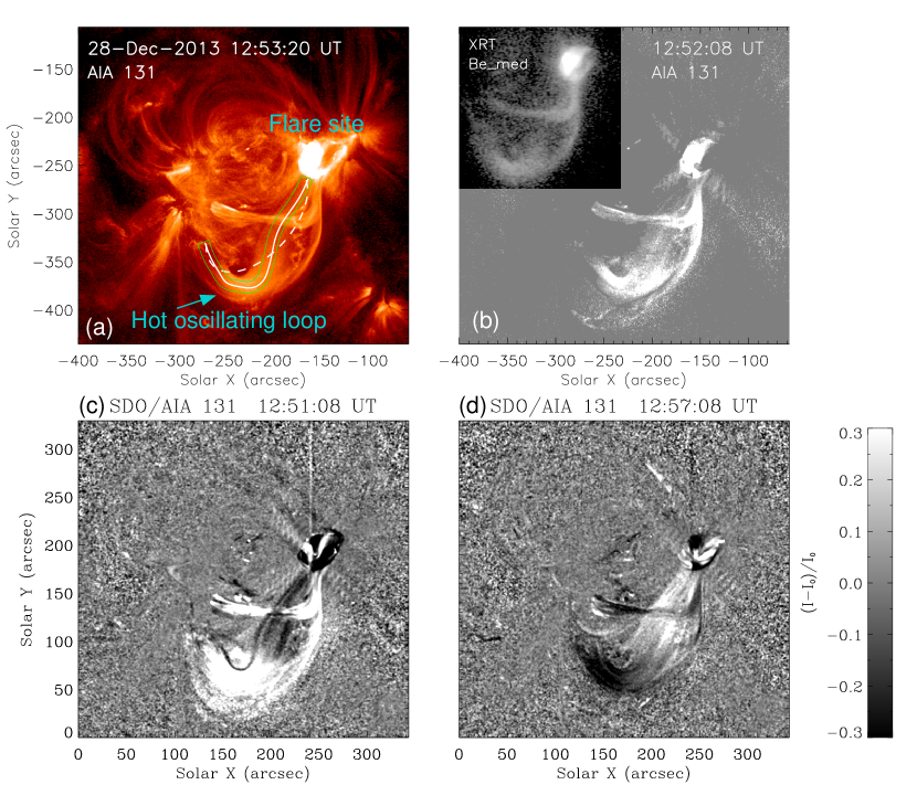
Figure 1.— Observations of a longitudinal wave event on 2013 December 28. (a) AIA 131 Å image. A sampled slice (green lines) along the oscillating loop is used to construct the time-distance plot shown in Figure 2. The white thick curve indicates the reconstructed 3D loop (same as the sampled track) and the dashed curve for a fitted circular model. (b) AIA 131 Å base-difference image relative to a pre-flare image at 12:40 UT. The inset shows a co-temporal Hinode/XRT image in the Be_med filter. (c) and (d): The detrended 131 Å images at 12:51 UT and 12:57 UT, showing the antiphase intensity perturbations at the opposite legs of the loop. (Animations are available in the online journal)

2. Observations and data analysis

A GOES C3.0-class flare occurred on 2013 December 28 in NOAA Active Region (AR) 11936 near disk center of the Sun. The flare began at 12:40 UT and peaked at 12:47 UT. This flare excited longitudinal waves in a heated loop observed with $SDO$/AIA. The AIA records the full Sun in ten extreme ultraviolet (EUV) and UV passbands with high spatio-temporal resolution and wide temperature coverage (log$T$=3.7–7.3; Lemen et al., 2012). We analyze the loop dynamics and thermal property using the AIA data.

The longitudinal waves were clearly detected in AIA 131 Å (dominated by Fe xxi, formed at $\sim$11 MK) band. The animation shows that a large loop that connected the flare site at one end (marked with a curved cut in Figure 1(a)) developed quickly and exhibited intensity oscillations along the loop. Similar emission features seen in the AIA 131 Å base-difference image and a co-temporal soft X-ray image (Figure 1(b)) observed by Hinode/XRT (Golub et al., 2007) indicate that the oscillating loop is hot. To emphasize the evolution of intensity perturbations, we processed the 131 Å images by subtracting the slowly-varying trend at each pixels, and then normalized the perturbation to the trend, where the trend was derived using the Fourier low-pass ($\geq$20 min) filtering. The detrended images show alternate intensity enhancements at the opposite legs with rapid decay (Figures 1(c) and (d)). The animation shows that the loop oscillations lasted for about two periods before they faded out.

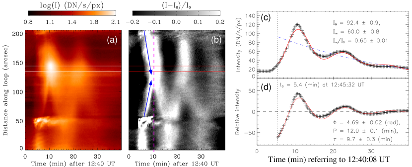
Figure 2.— Measurements of the loop oscillations seen in 131 Å. (a) Time-distance plot for the sample wave path traced out in Figure 1(a), showing wave perturbations along the loop. In the plot, the distance is measured from the end near the flare site. (b) Same as (a) but with the slowly-varying trend subtracted at each position. The two arrows marked indicate two initial brightenings propagating in the opposite directions. (c) Time profile of the average counts extracted from a 9-arcsec wide region (narrow box in (a)). The solid curve shows a best fit which includes a parabolic trend (dashed line). (d) Detrended light curve with the best fit (solid line).

To measure the wave properties we sampled the 131 Å images from a 21-pixel (13 arcsec) wide slice (outlined in Figure 1(a)) over a period of 12:40–13:20 UT. We averaged the slices over the width and stacked them in time to construct a time-distance plot (Figure 2(a)). Figure 2(b) shows the corresponding detrended time-distance plot. The intensity oscillations along each leg are nearly in-phase but anti-phase between the opposite legs matching the signature for a fundamental standing slow mode predicted by forward modelings (Taroyan & Bradshaw, 2008). Figure 2(c) shows the time profile of mean intensity for a cut selected at the leg with the brightest emission (at segment 15 shown in Figure 3(a)). We fitted the oscillatory signals with the function

$$I(t)=I_{m}{\rm sin}\left(\frac{2\pi(t-t_{0})}{P}+\phi\right){\rm exp}\left(-\frac{t-t_{0}}{\tau}\right)+I_{0}(t),$$ (1)

where $I_{m}$, $P$, $\tau$, $\phi$, and $t_{0}$ are the amplitude, period, decay time, initial phase, and reference time, respectively, and $I_{0}(t)$ is a parabolic trend. The best fits to the light curve with and without the trend are shown in Figures 2(c) and 2(d), respectively. The period of oscillation is $P=12.0\pm 0.1$ min, the decay time $\tau=9.7\pm 0.3$ min, and the initial amplitude relative to the trend is $I_{m}/I_{0}(t_{0})=0.65\pm 0.01$.

The phase speed is important for identification of wave modes, which requires an estimate of the loop length. We estimated the loop 3D geometry using the curvature radius maximization method which assumes the line-of-sight (LOS) coordinates of the observed loop to be the corresponding LOS coordinates of a circular model (Aschwanden et al., 2002; Aschwanden, 2009). Figure 1(a) shows the fitted circular model and the solution of the 3D geometry which has an identical 2D projection as observed. We obtained the loop length $L$=179 Mm, about 33 Mm longer than that of its 2D projection. The wave phase speed was estimated by $V_{p}$=2$L/P=500\pm 50$ km s^-1, where an uncertainty in $L$ is taken as $0.1L$. The phase speed is close to the sound speed of 480 km s^-1 for the loop temperature $T\sim$10 MK, estimated using $c_{s}=152T_{6}^{1/2}$ km s^-1, where $T_{6}=T$/[1 MK] and taking the adiabatic index $\gamma$=5/3. This result supports the interpretation of the observed waves as a fundamental slow mode.

To conduct accurate diagnostics of the electron temperature and density of the oscillating loop we utilized a regularized differential emission measure (DEM) analysis on AIA images in six EUV channels (94, 131, 171, 193, 211, and 335 Å) (Hannah & Kontar, 2012, 2013). As an illustration, we chose the images at $\sim$12:53 UT when the entire loop became obvious to trace, and divided the entire loop into 23 subsections (Figure 3(a)). We performed the DEM inversion for each segment and fitted the DEM curve with a triple-Gaussian model to separate a hot component ($\xi_{\rm hot}(T)$) from the background by assuming that the hot component comes from the foreground hot oscillating loop (Figures 3(b) and (h)). The application of this technique was detailed in Sun et al. (2013). Figures 3(d) and (e) show the loop temperature (the centroid of the hottest Gaussian component) and the loop emission measure ($EM=\int\xi_{\rm hot}(T)dT$, the pink area in Figure 3(b)). We measured the loop width by fitting the cross-sectional flux profile with a Gaussian function, and obtained the mean FWHM width, $w=13.8\pm 1.7$ Mm for segments 8–18 (Figure 3(f)). By using $n=\sqrt{EM/w}$ with a filling factor of unity (leading to a lower limit of $n$), the loop electron density was estimated (Figure 3(g)). Both the loop temperature and density are found to vary in a small range along the loop ($T$=7–12 MK and $n$=(1.6–3.0)$\times 10^{9}$ cm^-3).

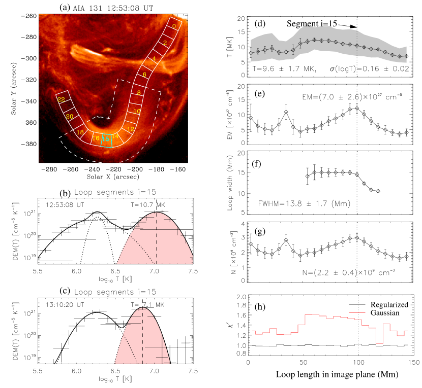
Figure 3.— The DEM analysis of loop thermal properties. (a) AIA 131 Å subimage of the analyzed loop. The traced loop is divided into 23 segments (solid lines) with segment $i$=0 near the flare site. Each segment has a size of 15$\times$21 pixels. A 70-pixels wide region outlined with dashed lines is selected for measuring the width of loop cross sections. The loop segment $i$=15 is used for the analysis of EM and temperature evolution shown in Fig. 4. Panels (b) and (c) show the regularized DEM inversion result for segment 15 at 12:53 UT and 17 min later. The DEM profile (crosses) is fitted to a triple-Gaussian model (curves) for isolating the foreground hot loop contribution (pink). (d) Loop temperature. The gray band shows the temperature range ($\pm\sigma_{T}$, Gaussian width in Log$T$). (e) Loop EM. (f) Loop width. (g) Electron density. (h) Reduced chi-squares ($\chi^{2}$) for the regularized DEM and the Gaussian model in data space. Error bars in (d)-(g) are the 1$\sigma$ fitting error. (An animation is available in the online journal)

To study the time evolution of thermal properties, we focused on segment 15 with the maximum EM and used its average flux in six AIA bands to perform a time series of DEM inversions with a cadence of 24 s. By applying the triple-Gaussian DEM analysis (Figures 3(b) and (c) and the animation in the online version), we obtained time profiles of the loop temperature and electron density (Figures 4(a) and (b)), where the loop width $w$ was taken as a constant ($\sim$14 Mm) in calculation of the density evolution. The mean temperature over the lifetime of oscillations is found to be $T=8.7\pm 1.7$ MK, and the mean density $n=(2.6\pm 0.2)\times 10^{9}$ cm^-3. The wave signals in measured temperature and density are evident. We fitted the oscillations with a damped sine-function of the same form as equation (1). The fitted oscillations and the background trends are shown in Figures 4(a) and (b). The detrended oscillations with the fitted parameters are shown in Figures 4(c) and (d). We find that the temperature and density oscillations have similar periods and they are nearly in phase. The initial phase shift is $\Delta\phi=6^{\circ}\pm 23^{\circ}$. The phase shift measured using the cross correlation from the relative perturbations to the trend is about 12^∘.

Under the polytropic assumption $p\sim n^{\alpha}$ with a polytropic index $\alpha$, it can be derived from linearized ideal MHD theory that (e.g. Van Doorsselaere et al., 2011):

$$\frac{T^{{}^{\prime}}}{T_{0}}=(\alpha-1)\frac{n^{{}^{\prime}}}{n_{0}},$$ (2)

where $p$, $n$, $T$ are the gas pressure, electron number density, and temperature, respectively. A superscript (${}^{{}^{\prime}}$) indicates perturbed quantities and a subscript (₀) stands for equilibrium quantities. The process is adiabatic only if $\alpha$=$\gamma$=5/3. The polytropic index can be measured using the linear relationship between the observables $T^{{}^{\prime}}/T_{0}$ and $n^{{}^{\prime}}/n_{0}$. Note that the equation (2) does not generally hold true in the nonideal MHD case. For example, thermal conduction can lead a large phase shift between $T^{{}^{\prime}}$ and $n^{{}^{\prime}}$ (see the discussion in Section 3). In this case, the polytropic index should be measured either using equation (2) for the data after removing the phase shift, or based on the wave amplitude measurements as

$$\alpha=\frac{A_{T}(t)}{A_{n}(t)}+1,$$ (3)

where $A_{T}(t)$ and $A_{n}(t)$ are the decaying temperature and density amplitudes normalized to the corresponding trend. Here we chose equation (2) to measure the polytropic index because the observed temperature and density perturbations are nearly in phase and the advantage compared to using equation (3) is that the assumption of the oscillations as a damped sine-function is not required. We obtained $\alpha=1.64\pm 0.08$ using the linear least-squares fitting to the scatter plot of the data ($T^{{}^{\prime}}/T_{0}(t)$ and $N^{{}^{\prime}}/N_{0}(t)$) over the wave lifetime of 12:46–13:20 UT (Figure 5(a)), and obtained $\alpha=1.66\pm 0.09$ by fitting only the data within the first oscillation period (Figure 5(b)). We find that the value of $\alpha$ agrees well with the adiabatic index of 5/3 for fully ionized coronal plasmas. Note that the assumptions of the line-of-sight column depth and the filling factor used in determination of the loop density from EM have little effect on the accuracy of the measurement because $\alpha$ depends only on the relative perturbations of the density ($n^{{}^{\prime}}/n_{0}$).

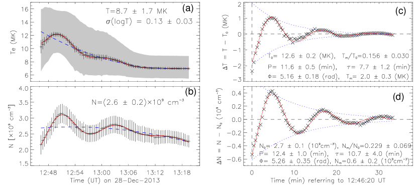
Figure 4.— Evolution of thermal properties for the loop segment 15. (a) Temperature. The red solid curve shows the best fit to the oscillatory signals, and the dashed curve is the parabolic trend. (b) Same as (a) but for electron density. The gray band and error bars in (a) and (b) have same meanings as in Figure 3. (c) Detrended time profile of the temperature (crosses) and the best fit (red curve). (d) Same as (c) but for electron density.

3. Discussion and Conclusions

We have studied a non-eruptive flare event (not associated with a CME) occurring near one footpoint of a large coronal loop observed by SDO/AIA. The flare impulsively heats the loop to above 10 MK and also generates the longitudinal waves in the hot loop. Despite of difficulties in distinguishing propagating and standing waves based on only intensity information, we argue that the observed wave is most likely of a fundamental standing slow mode. This is suggested by the signature that the temperature and density oscillations match well a harmonic wave with the frequency close to that for the fundamental mode. In contrast, a reflecting single wave pulse does not follow a sine-function in temporal variation and its time distance plot exhibits a ‘zigzag’ pattern (De Moortel & Hood, 2003; Taroyan & Bradshaw, 2008; Kumar et al., 2013). In addition, the nearly inphase intensity oscillations shown along each leg after $\sim$12:50 UT suggest that the standing wave appears to form within one wave period after the flare, consistent with the case of standing slow waves observed by SOHO/SUMER (Wang et al., 2003a, 2005). The quick setup of the standing wave could be related to meeting of the two oppositely-propagating brightenings (marked with arrows in Figure 2(b)) in the initial phase (Selwa & Ofman, 2009), however, a detailed study on the wave excitation is beyond the scope of this Letter.

Here, we focus our analyses on the plasma thermal and wave properties of the hot loop, and have measured the polytropic index $\alpha$ from the temperature and electron density perturbations. We find that the value of $\alpha$ is close to 5/3 within a small uncertainty particularlly in the first oscillation period. This is striking because it implies that the energy equation in the MHD equations can be well represented with an adiabatic form, or the non-ideal effects such as energy gain and losses on the timescale of oscillations are negligible in the hot plasma of $T\gtrsim$9 MK. The reasons are detailed in the following based on the linearized 1D hydrodynamic equations including the effects of gravity, heat conduction, compressive viscosity, and optically thin radiative losses and gains (e.g., De Moortel & Hood, 2003; Sigalotti et al., 2007). Note that both the measurements of $\alpha$ and the theoretical interpretations below are independent on whether the observed slow wave is of propagating or standing mode because they are essentially identical in physical property.

(1) We know that for an isothermal loop in hydrostatic equilibrium, the pressure scale height $H=50T_{6}$ Mm. For the hot loop at $T\approx$9 MK, we have $H/h\approx$9 where $h$=50 Mm, the estimated loop height. Thus the stratification effect here can be neglected.

(2) We estimate the effect of radiative loss from the ratio of the oscillation period to the radiation time scale $r=P/\tau_{\rm rad}$. Here $\tau_{\rm rad}=3450n_{9}^{-1}T_{6}^{3/2}$ s, where $n_{9}=n/[10^{9}{\rm cm}^{-3}$] (Sun et al., 2013). For the measured parameters $T$=8.7 MK, $n=2.6\times 10^{9}$ cm^-3 and $P$=12 min, we obtain $\tau_{\rm rad}\approx$570 min and $r\approx$0.02. Thus radiative cooling is negligible on the oscillation period timescale.

(3) It is known that when thermal conduction dominates in the energy equation, it introduces a phase shift ($\Delta{\phi}$) between the density and temperature perturbations (Owen et al., 2009; Van Doorsselaere et al., 2011). The linear approximation gives the following relations

$${\rm tan}\Delta{\phi} = \frac{\pi(\gamma-1)\kappa_{\|}}{k_{B}c_{s}^{2}Pn},$$ (4)

$$\frac{A_{T}}{A_{n}} = (\gamma-1){\rm cos}\Delta\phi~{}~{}~{}[=\,\alpha-1],$$ (5)

where $\gamma$=5/3, $k_{B}$ the Boltzmann constant, $\kappa_{\|}=7.8\times 10^{-7}T^{5/2}$ ergs cm^-1s^-1K^-1 the thermal conductivity parallel to the magnetic field (Spitzer, 1962). Note that the above equations hold true no matter whether thermal conduction or compressive viscosity dominates in the wave damping (see item (4)). 1D MHD simulations have shown the presence of a large phase shift between $T^{{}^{\prime}}$ and $n^{{}^{\prime}}$ in hot loops due to thermal conduction (e.g. Ofman & Wang, 2002; Sigalotti et al., 2007).

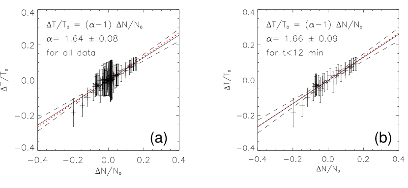
Figure 5.— Measurements of the polytropic index $\alpha$. (a) The scatter plot of electron density and temperature perturbations (pluses), with the best-fitting line (solid) and the line of $\gamma$=5/3 (dotted). The dashed lines indicate the $\pm 1\sigma$ fitting error. (b) Same as (a) but for the data within 12 min after 12:46:20 UT.

However, we find that the temperature and density oscillations are nearly in phase. This result suggests that the thermal conduction may be much weaker than the classical theory predicted in the hot flaring loop. With the loop parameters used in item (2) we obtain the theory-predicted $\Delta{\phi}=35^{\circ}$ using equation (4). The comparison of the observed phase shift ($\sim 12^{\circ}$) with the predicted suggests a reduction of (parallel) thermal conductivity by a factor of three. Moreover, from the measured polytropic index of $\alpha$=1.64 we derive the phase shift to be $\sim 16^{\circ}$ using equation (5), which is consistent with the directly measured value. Thus both the phase shift and polytropic index measurements support the conduction suppression in this event. In addition, the results of $\alpha$=1.66 that is even closer to $\gamma$=5/3 and a better in-phase relationship between $T^{{}^{\prime}}$ and $n^{{}^{\prime}}$ within the first oscillation period suggest that thermal conduction tends to be more suppressed when the plasma is hotter ($T\gtrsim$9 MK).

In addition, we notice that for hot loop oscillations observed by SUMER and SDO/AIA (Wang et al., 2003a, 2007; Kumar et al., 2013, 2015), the measured phase speeds are close to the adiabatic sound speed within uncertainties, also suggesting $\alpha\sim$5/3. This is in contrast to the theoretical prediction from linear MHD simulations by De Moortel & Hood (2003). They showed that when thermal conduction is dominant due to the high temperatures, the perturbations propagate largely undamped, at the slower, isothemal sound speed, which implies $\alpha\sim$1.

(4) In using equation (2) to measure the polytropic index, we have assumed that the loop temperature (or sound speed) varies gradually with time relative to the wave period (known as the WKB approximation). To check its validity, we quantify the “gradual variation” as the requirement that changes in wave period must be small over a single period. The condition can be expressed as $|dP/dt|\ll 1$. The fitting to the evolution of the loop temperature (Figure 4(a)) gives the trend, $T(t)=T_{0}+at+bt^{2}$, where the initial temperature $T_{0}$=12.6 MK, the polynomial coefficients $a$=$-$0.38 MK min^-1 and $b$=0.0064 MK min^-2. Considering $P(t)=2L/c_{s}(T(t))$, we obtain $|dP/dt|=P_{0}T_{0}^{1/2}|0.5a+bt|T(t)^{-3/2}$, where $P_{0}=2L/c_{s}(T_{0})$=10.5 min. The calculation of its maximum value $|dP/dt|_{\rm max}$=0.16 indicates that the WKB approximation is valid in this case. This justifies the removal of the trend from the oscillations in our analysis.

(5) As the viscous heating belongs to the second-order term in the linearized energy equation, its effect on wave damping can be neglected. Thus the only dominant damping mechanism left is the momentum loss by the viscous forces. From the dispersion relation derived from the velocity wave equation when only compressive viscosity is present (see Eq.(33) in Sigalotti et al., 2007), we can obtain the coefficient of compressive viscosity in terms of the observables by

$$\eta_{s}=\frac{3\gamma p_{0}\tau}{8\pi^{2}(\tau/P)^{2}+2}=\frac{3\gamma k_{B}n_{0}T_{0}\tau}{4\pi^{2}(\tau/P)^{2}+1},$$ (6)

where $\gamma$=5/3 and $p_{0}=2n_{0}k_{B}T_{0}$. By taking $P=12.0\pm 0.6$ min and $\tau=9.2\pm 2.1$ min (the mean for temperature and density oscillations) with $T_{0}=8.7\pm 1.7$ MK and $n_{0}=(2.6\pm 0.2)\times 10^{9}$ cm^-3, we obtain $\eta_{s}=356\pm 195$ g cm^-1 s^-1. In comparison, we calculate the classical Braginskii compressive viscosity coefficient using $\eta_{0}=0.1T_{6}^{5/2}$ g cm^-1 s^-1 (e.g., Ofman & Wang, 2002), and obtain $\eta_{0}\approx 23$ g cm^-1 s^-1, thus, $\eta_{s}/\eta_{0}=15$. This implies that to interpret the wave damping timescale by the compressive viscosity alone the classical viscosity coefficient needs to be enhanced by a factor of 15, which may be regarded as an upper limit considering the additional effects such as weak nonlinearity, thermal conduction and stratification.

In summary, we have found quantitative evidence of thermal conduction suppression in a hot flare loop by coronal seismology of the slow-mode waves. This result suggests that the flare loop should cool much slower than expected from the classical Spitzer conductive cooling. Our studied event is indeed of such long-duration events (LDEs) which are the flares with a slower-than-expected decay rate in soft X-ray and EUV radiation (e.g., Forbes & Acton, 1996; Takahashi & Watanabe, 2000; Qiu et al., 2012). To explain the LDEs and flare loop-top sources, some previous studies have suggested the mechanism of continuous heating (Warren, 2006; Liu et al., 2013; Sun et al., 2013) or conduction suppression (McTiernan et al., 1993; Jiang et al., 2006; Li et al., 2012). Our study confirms the effect of the latter mechanism in a more direct way. Laboratory experiments and numerical studies showed that the actual conductivity is smaller (by at least a factor of two) than that given by Spitzer when $l\lesssim 30\lambda$ where $l$ is the temperature gradient scale length and $\lambda$ the mean free path of thermal electrons (Bell et al., 1981; Luciani et al., 1983). We estimate $l/\lambda\sim 30$ in this case, suggesting that the nonlocal conduction may account for the observed conduction suppression (Matte & Virmont, 1982; Rosner et al., 1986). By studying the evolution of flare loop-top sources, Jiang et al. (2006) suggested that plasma waves or turbulence may play an important role in suppressing the conduction during the decay phase of flares. The mechanism is similar to that used for interpreting the significant reduction of thermal conductivity in galaxy-cluster cooling flows by a tangled magnetic field (Chandran & Cowley, 1998). Finally, we conclude that the result of conduction suppression may also shed light on the coronal heating problem (see the review by Klimchuk, 2015), because weak thermal conductivity implies smaller conductive losses, and an extended lifetime of individual nanoflares, increasing the average coronal temperature for the same heating rate.

The work of T. W. was supported by NASA grants NNX12AB34G and the NASA Cooperative Agreement NNG11PL10A to CUA. L. O. and E. P. acknowledge to support from the NASA grant NNX12AB34G. SDO is a mission for NASA’s Living With a Star (LWS) program.

References

- Al-Ghafri et al. (2014) Al-Ghafri, K. S., Ruderman, M. S., Williamson, A., & Erdélyi, R. 2014, ApJ, 786, 36
- Aschwanden et al. (2002) Aschwanden, M. J., Pontieu, B. D., Schrijver, C. J., & Title, A. 2002, Sol. Phys., 206, 99
- Aschwanden (2009) Aschwanden, M. J. 2009, Space Sci. Rev., 149, 31
- Bell et al. (1981) Bell, A. R., Evans, R. G., & Nicholas, D. J. 1981, Phys. Rev. Lett., 46, 243
- Chandran & Cowley (1998) Chandran, B. D. G., & Cowley, S. C. 1998, Phys. Rev. Lett., 80, 3077
- De Moortel & Hood (2003) De Moortel, I., & Hood, A.W. 2003, A&A, 408, 755
- De Moortel & Nakariakov (2012) De Moortel, I., & Nakariakov, V. M. 2012, Phil. Trans. R. Soc. A, 370, 3193
- Forbes & Acton (1996) Forbes, T. G., & Acton, L. W. 1996, ApJ, 459, 330
- Golub et al. (2007) Golub, L., Deluca, E., Austin, G., et al. 2007, Sol. Phys., 243, 63
- Hannah & Kontar (2012) Hannah, I. G., & Kontar, E. P. 2012, A&A, 539, A146
- Hannah & Kontar (2013) Hannah, I. G., & Kontar, E. P. 2013, A&A, 553, A10
- Jacobs & Poedts (2011) Jacobs, C., & Poedts, S. 2011, Adv. Space Res., 48, 1958
- Jiang et al. (2006) Jiang, Y., Liu, S., Liu, W., & Petrosian, V. 2006, ApJ, 638, 1140
- Klimchuk (2015) Klimchuk, J. 2015, Phil. Trans. R. Soc. A, 373, 20140256
- Kumar et al. (2013) Kumar, P. , Innes, D. E., & Inhester, B. 2013, ApJ, 779, L7
- Kumar et al. (2015) Kumar, P. Kumar, P., Nakariakov, V. M., & Cho, K.-S., ApJ, 804, 4
- Lemen et al. (2012) Lemen, J. R., Title, A. M., Akin, D. J., et al. 2012, Sol. Phys., 275, 17
- Li et al. (2012) Li, T. C., Drake, J. F., & Swisdak, M. 2012, ApJ, 757, 20
- Liu & Ofman (2014) Liu, W., & Ofman, L. 2014, Sol. Phys., 289, 3233
- Liu et al. (2013) Liu, W.-J., Qiu, J., Longcope, D. W., & Caspi, A. 2013, ApJ, 770, 111
- Luciani et al. (1983) Luciani, J. F., Mora, P., & Virmont, J. 1983, Phys. Rev. Lett., 51, 1664
- Matte & Virmont (1982) Matte, J. P., & Virmont, J. 1982, Phys. Rev. Lett., 49, 1936
- McTiernan et al. (1993) McTiernan, J. M., Kane, S. R., Loran, J. M., et al. 1993, ApJ, 416, L91
- Nakariakov & Verwichte (2005) Nakariakov, V.M., Verwichte, E. 2005, Living Rev. in Sol. Phys., 2, 3
- Ofman & Wang (2002) Ofman, L., & Wang, T. J. 2002, ApJ, 580, L85
- Ofman et al. (2012) Ofman, L., Wang, T. J., & Davila, J. M. 2012, ApJ, 754, 111
- Owen et al. (2009) Owen, N. R., De Moortel, I., & Hood, A. W. 2009, A&A, 494, 33
- Pudovkin et al. (1997) Pudovkin, M. I., Meister, C.-V., Besser, B. P., & Biernat, H. K. 1997, J. Geophys. Res., 102, 27145
- Qiu et al. (2012) Qiu, J., Liu, W.-J., & Longcope, D. W. 2012, ApJ, 752, 124
- Riley et al. (2001) Riley, P., Gosling, J. T., & Pizzo, V. J. 2001, J. Geophys. Res., 106, 8291
- Roberts et al. (1983) Roberts, B., Edwin, P. M., & Benz, A. O. 1983, Nature, 305, 688
- Rosner et al. (1986) Rosner, R., Low, B. C., & Holzer, T. E. 1986, in Physics of the Sun. II, ed. P. A. Sturrock (Dordrecht: Reidel), 135
- Ruderman (2013) Ruderman, M. S. 2013, A&A, 553, A23
- Selwa & Ofman (2009) Selwa, M., & Ofman, L. 2009, Ann. Geophys., 27, 3899
- Shibata & Yokoyama (2002) Shibata, K., & Yokoyama, T. 2002, ApJ, 577, 422
- Sigalotti et al. (2007) Sigalotti, L. Di G., Mendoza-Briceño, C. A., & Luna-Cardozo, M. 2007, Sol. Phys., 246, 187
- Spitzer (1962) Spitzer, L., Jr. 1962, Physics of Fully Ionized Gases (New York: Wiley Interscience)
- Sun et al. (2013) Sun, X., Hoeksema, J. T., Liu, Y., et al. 2013, ApJ, 778, 139
- Takahashi & Watanabe (2000) akahashi, M., & Watanabe, T. 2000, Adv. Space Res., 25, 1833
- Taroyan & Bradshaw (2008) Taroyan, Y., & Bradshaw, S. 2008, A&A, 481, 247
- Van Doorsselaere et al. (2011) Van Doorsselaere, T., Wardle, N., Del Zanna, G., et al. 2011, ApJ, 727, L32
- Wang (2011) Wang, T. J. 2011, Space Sci. Rev., 158, 397
- Wang et al. (2002) Wang, T., Solanki, S. K., Curdt, W., Innes, D. E., & Dammasch, I. E. 2002, ApJ, 574, L101
- Wang et al. (2003a) Wang, T. J., Solanki, S. K., Innes, D. E., Curdt, W., & Marsch, E. 2003a, A&A, 402, L17
- Wang et al. (2003b) Wang, T. J., Solanki, S. K., Curdt, W., et al. 2003b, A&A, 406, 1105
- Wang et al. (2005) Wang, T. J., Solanki, S. K., Innes, D. E., & Curdt, W. 2005, A&A, 435, 753
- Wang et al. (2007) Wang, T. J., Innes, D. E., & Qiu, J. 2007, ApJ, 656, 598
- Warren (2006) Warren, H. P. 2006, ApJ, 637, 522