Topological Properties of Electrons in Honeycomb Lattice with Kekulé Hopping Textures

Abstract

Honeycomb lattice can support electronic states exhibiting Dirac energy dispersion, with graphene as the icon. We propose to derive nontrivial topology by grouping six neighboring sites of honeycomb lattice into hexagons and enhancing the inter-hexagon hopping energies over the intra-hexagon ones. We reveal that this manipulation opens a gap in the energy dispersion and drives the system into a topological state. The nontrivial topology is characterized by the $\mathbb{Z}_{2}$ index associated with a pseudo time-reversal symmetry emerging from the $C_{6}$ symmetry of the Kekulé hopping texture, where the angular momentum of orbitals accommodated on the hexagonal ”artificial atoms” behaves as the pseudospin. The size of topological gap is proportional to the hopping-integral difference, which can be larger than typical spin-orbit couplings by orders of magnitude and potentially renders topological electronic transports available at high temperatures.

I Introduction

Honeycomb lattice can host electrons with Dirac-like linear dispersion due to its $C_{3}$ crystal symmetry Wallace1947 , and interests in questing for systems with honeycomb lattice structure flourished since the discovery of graphene produced by the scotch-tape technique Novoselov2004 ; GrapheneBook ; Geim2009 . The Dirac dispersion and the associated chiral property of electronic wave functions accommodated on honeycomb lattice make it an ideal platform for exploring topological states QHE ; TKNN without external magnetic field. It was shown first that a quantum anomalous Hall effect (QAHE) can be realized when complex hopping integrals among next-nearest-neighboring sites of honeycomb lattice are taken into account Haldane1988 . Later on it was revealed that the intrinsic spin-orbit coupling (SOC) in honeycomb lattice can provide this complex hopping integrals, which drives spinful electrons into a topological state with preserved time-reversal (TR) symmetry, known as quantum spin Hall effect (QSHE) KaneRMP ; ZhangRMP ; Kane2005a ; Kane2005b . Quite a number of activities have been devoted towards realizing topological states in electron systems on honeycomb lattice, such as QAHE by straining GeimNPhys2010 ; Gomes2012 , twisting Hunt2013 ; He2013 and decorating graphene QNiuPRB2010 , and QAHE with spin-polarized edge currents in terms of the antiferromagnetic exchange field and staggered electric potential LiangNJP2013 . Honeycomb lattice can also be tuned to support topological states in photonic crystals Haldane2008 ; Wu2015 and cold atoms Tarruell2012 .

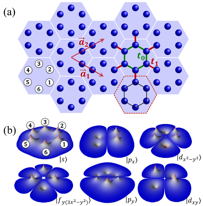
Figure 1: (Color online) (a) Honeycomb lattice with a Kekulé texture in hopping energies between NN sites: $t_{0}$ inside hexagons as denoted by the green bonds and $t_{1}$ between hexagons by red ones. The Red dashed hexagon is the primitive cell of triangular lattice with lattice vectors $\vec{a}_{1}$, $\vec{a}_{2}$ and lattice constant $a_{0}=|\vec{a}_{1}|=|\vec{a}_{1}|$. Numbers $1,\dots,6$ in circle index atomic sites within a hexagon. (b) Emergent orbitals in the hexagonal artificial atom.

In the present work, we explore possible topological properties in honeycomb lattice by introducing a Kekulé texture in hopping energy between nearest-neighboring (NN) sites. We take a hexagonal primitive unit cell and view the honeycomb lattice as a triangle lattice of hexagons [see the dashed red line in Fig. 1(a)]. When the inter-hexagon hopping $t_{1}$ is tuned to be larger than the intra-hexagon one $t_{0}$, a topological gap is opened at the $\Gamma$ point accompanied by a band inversion between orbitals with opposite spatial parities accommodated on hexagons [see Fig. 1(b)]. A pseudo-TR symmetry associated with a pseudospin degree of freedom and Kramers doubling in the emergent orbitals are revealed based on $C_{6}$ point group symmetry, which generates the $\mathbb{Z}_{2}$ topology. For experimental implementations, we discuss that, along with many other possibilities, the molecular graphene realized by placing carbon monoxides (CO) periodically on Cu [111] surface Gomes2012 is a very promising platform to realize the present idea, where the Kekulé texture can be controlled by adding extra CO molecules.

The paper is organized as follows. In Sec. II, we start with a $C_{6}$ symmetric Kekulé hopping texture among NN sites in honeycomb lattice, where a pseudo-TR symmetry and pseudospin emerge. In Sec. III, we derive an effective low-energy Hamiltonian of the system and reveal the $\mathbb{Z}_{2}$ topology. The topological properties of the system is demonstrated by the edge state and associated Hall and longitudinal conductances in sections  IV and V. We discuss a promising experimental platform for realizing the topological state in Sec. VI. Concluding remarks are presented in Sec. VII.

II Kekulé hopping texture and emergent orbitals

We start from a spinless tight-binding Hamiltonian on honeycomb lattice

$$H=\varepsilon_{0}\sum_{i}c_{i}^{\dagger}c_{i}+t_{0}\sum_{\langle i,j\rangle}c_{i}^{\dagger}c_{j}+t_{1}\sum_{\langle i^{\prime},j^{\prime}\rangle}c_{i^{\prime}}^{\dagger}c_{j^{\prime}},$$ (1)

with $c_{i}$ the annihilation operator of electron at atomic site $i$ with on-site energy $\varepsilon_{0}$ satisfying anti-commutation relations, $\langle i,j\rangle$ and $\langle i^{\prime},j^{\prime}\rangle$ running over NN sites inside and between hexagonal unit cells with hopping energies $t_{0}$ and $t_{1}$ respectively [see Fig. 1(a)]. The orbitals are considered to be the simplest one without any internal structure, same as the $\pi$ electron of graphene. Below we are going to detune the hopping energy $t_{1}$ while keeping $t_{0}$ constant, and elucidate possible changes in the electronic state. In this case, the pristine honeycomb lattice of individual atomic sites is better to be considered as a triangular lattice of hexagons, with the latter characterized by $C_{6}$ symmetry.

Let us start with the Hamiltonian within a single hexagonal unit cell

$$H_{0}=t_{0}\Psi^{\dagger}\left(\begin{array}[]{cccccc}0&1&0&0&0&1\\ 1&0&1&0&0&0\\ 0&1&0&1&0&0\\ 0&0&1&0&1&0\\ 0&0&0&1&0&1\\ 1&0&0&0&1&0\end{array}\right)\Psi,$$ (2)

where $\Psi=[c^{1},c^{2},c^{3},c^{4},c^{5},c^{6}]^{T}$ [see Fig. 1(a)]. The eigenstates of Hamiltonian $H_{0}$ are given by

$$|s\rangle=[1,1,1,1,1,1]^{T};$$

$$|p_{x}\rangle=[1,1,0,-1,-1,0]^{T};$$

$$|p_{y}\rangle=[1,-1,-2,-1,1,2]^{T};$$

$$|d_{x^{2}-y^{2}}\rangle=[1,1,-2,1,1,-2]^{T};$$

$$|d_{xy}\rangle=[1,-1,0,1,-1,0]^{T};$$

$$|f_{y(3x^{2}-y^{2})}\rangle=[1,-1,1,-1,1,-1]^{T}$$ (3)

with eigenenergies $2t_{0},t_{0},t_{0},-t_{0},-t_{0}$ and $-2t_{0}$ respectively, up to normalization factors. As shown in Fig. 1(b), the emergent orbitals accommodated on the hexagonal “artificial atom” take the shapes similar to the conventional $s$, $p$, $d$ and $f$ atomic orbitals in solids.

A pseudo-TR symmetry operator can be composed in the present system with $C_{6}$ symmetry: $\mathcal{T}=\mathcal{UK}$ with $\mathcal{K}$ the complex conjugate operator and $\mathcal{U}=-i\sigma_{y}$, where $\sigma_{y}$ is the Pauli matrix. It can be checked straightforwardly that $\mathcal{U}$ corresponds to $\pi/2$ rotation for $p$ orbitals and $\pi/4$ rotation for $d$ orbitals given in Eq. (3), which yields $\mathcal{U}^{2}=-1$ in the space formed by the $p$ and $d$ orbitals Wu2015 . Therefore, the pseudo-TR symmetry satisfies the relation $\mathcal{T}^{2}=-1$, which is same as that for fermionic particles even though the spin degree of freedom of electron has not been considered here. This indicates that electrons acquire a new pseudospin degree of freedom in the present system as far as the low-energy physics is concerned.

Explicitly the wave functions carrying pseudospins are given by the emergent orbitals with eigen angular momentum

$$|p_{\pm}\rangle=\frac{1}{\sqrt{2}}\left(|p_{x}\rangle\pm i|p_{y}\rangle\right);|d_{\pm}\rangle=\frac{1}{\sqrt{2}}\left(|d_{x^{2}-y^{2}}\rangle\pm i|d_{xy}\rangle\right).$$ (4)

Distinguished from the intrinsic spin, the pseudospin is directly related to the chiral current density on the hexagon. For a lattice model, the current density between two sites is given by $I_{jk}=(i/\hbar)[t_{0}c_{j}^{\dagger}c_{k}-t_{0}^{*}c_{k}^{\dagger}c_{j}]$. The current distributions evaluated using wave functions in Eq. (4) for the pseudospin-up and -down states are shown in Figs. 2(a) and (b) with anticlockwisely and clockwisely circulating currents. By considering the hexagonal artificial atoms composed by six sites in honeycomb lattice, one harvests states with angular momentum merely from simple orbitals, such as $\pi$ electrons in graphene. The pseudo-TR symmetry is supported by the $C_{6}$ crystal symmetry, sharing the same underlying physics with the topological crystalline insulator FuPRL2011 . However, crystal-symmetry-protected topological insulators addressed so far need strong SOCs to achieve band inversions Hsieh2012 ; Dziawa2012 ; Xu2012 , which is different from the present approach as revealed below.

III Topological phase transition

We calculate the energy dispersion of Eq. (1) for several typical values of $t_{1}$ (hereafter the on-site energy is put as $\varepsilon_{0}=0$ without losing generality). As shown in Fig. 2, there are two two-fold degeneracies at the $\Gamma$ point corresponding to the two two-dimensional (2D) irreducible representations of $C_{6}$ point group. Projecting the wave functions for $t_{1}=0.9t_{0}$ onto the orbitals given in Fig. 1(b), it is found that the topmost two valance bands show the character of $d$ orbitals whereas the lowest two conduction bands behave like $p$ orbitals [see Fig. 2(c)], with the order in energy same as those listed in Eq. (3). For $t_{1}=t_{0}$, the $d$ and $p$ bands become degenerate at the $\Gamma$ point and double Dirac cones appear [see Fig. 2(d)], which are equivalent to the ones at $K$ and $K^{\prime}$ points in the unfolded Brillouin zone of honeycomb lattice with the rhombic unit cell of two sites. When $t_{1}$ increases further from $t_{0}$, a band gap reopens at the $\Gamma$ point. As shown in Fig. 2(e) for $t_{1}=1.1t_{0}$, the valence (conduction) bands are now occupied by $p$ ($d$) orbitals around the $\Gamma$ point, opposite to the order away from the $\Gamma$ point, and to that before gap closing. Therefore, a band inversion between $p$ and $d$ orbitals takes place at the $\Gamma$ point when the inter-hexagon hopping energy is increased across the topological transition point $t_{1}=t_{0}$, namely the pristine honeycomb lattice.

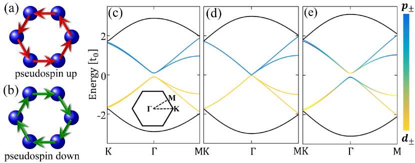
Figure 2: (Color online) (a) and (b) Current densities in the pseudospin-up channel ($p_{+}$ or $d_{+}$) and pseudospin-down channel ($p_{-}$ or $d_{-}$) respectively. Band dispersions for the system given in Fig. 1: (c) $t_{1}=0.9t_{0}$ (Inset: Brillouin zone of the triangular lattice), (d) $t_{1}=t_{0}$ and (e) $t_{1}=1.1t_{0}$. Blue and yellow are for $|p_{\pm}\rangle$ and $|d_{\pm}\rangle$ orbitals respectively, and rainbow for hybridization between them. The on-site energy is taken $\varepsilon_{0}=0$.

We can characterize the topological property of the gap-opening transition shown in Fig. 2 by a low-energy effective Hamiltonian around the $\Gamma$ point. Since the bands near Fermi level are predominated by $p$ and $d$ orbitals, it is sufficient to downfold the six-dimensional Hamiltonian $H(\mathbf{k})$ associated with the tight-binding model (1) into the four-dimensional subspace $[p_{+},d_{+},p_{-},d_{-}]$. The second term in Eq. (1) is then simply given by

$$h_{0}^{\prime}=\left(\begin{array}[]{cccc}t_{0}&0&0&0\\ 0&-t_{0}&0&0\\ 0&0&t_{0}&0\\ 0&0&0&-t_{0}\end{array}\right),$$ (5)

in the four-dimensional subspace. Contributions from the third term in Eq. (1) to the effective Hamiltonian should be evaluated perturbatively. First, we list the inter-hexagon hoppings in terms of 6$\times$6 matrices $h_{1},h_{2},h_{3},h_{1}^{\dagger},h_{2}^{\dagger}$ and $h_{3}^{\dagger}$ with

$$h_{1}=\left(\begin{array}[]{cccccc}0&0&0&t_{1}&0&0\\ 0&0&0&0&0&0\\ 0&0&0&0&0&0\\ 0&0&0&0&0&0\\ 0&0&0&0&0&0\\ 0&0&0&0&0&0\\ \end{array}\right),h_{2}=\left(\begin{array}[]{cccccc}0&0&0&0&0&0\\ 0&0&0&0&t_{1}&0\\ 0&0&0&0&0&0\\ 0&0&0&0&0&0\\ 0&0&0&0&0&0\\ 0&0&0&0&0&0\\ \end{array}\right),$$

$$h_{3}=\left(\begin{array}[]{cccccc}0&0&0&0&0&0\\ 0&0&0&0&0&0\\ 0&0&0&0&0&t_{1}\\ 0&0&0&0&0&0\\ 0&0&0&0&0&0\\ 0&0&0&0&0&0\\ \end{array}\right)$$

on the basis of $[c^{1},c^{2},c^{3},c^{4},c^{5},c^{6}]$. Following the standard procedures Sakurai , they can be projected to the subspace spanned by $[p_{+},d_{+},p_{-},d_{-}]$

$$h_{1}^{\prime} = \frac{t_{1}}{12}\left(\begin{array}[]{cccc}-2&\sqrt{3}-i&-1-\sqrt{3}i&2i\\ -\sqrt{3}-i&2&-2i&-1+\sqrt{3}i\\ -1+\sqrt{3}i&-2i&-2&\sqrt{3}+i\\ 2i&-1-\sqrt{3}i&-\sqrt{3}+i&2\end{array}\right),$$ (10)

$$h_{2}^{\prime} = h_{1}^{\prime*},$$

$$h_{3}^{\prime} = \frac{t_{1}}{6}\left(\begin{array}[]{cccc}-1&i&1&i\\ i&1&-i&1\\ 1&-i&-1&-i\\ i&1&-i&1\end{array}\right).$$ (15)

With Fourier transformations of matrices in Eqs. (5) and (15), one obtains the effective low-energy Hamiltonian $H^{\prime}(\mathbf{k})$ on the basis $[p_{+},d_{+},p_{-},d_{-}]$ in the momentum space. Expanding $H^{\prime}(\mathbf{k})$ around the $\Gamma$ point up to the lowest-orders of $\mathbf{k}$, one arrives at

$$H^{\prime}(\mathbf{k}\rightarrow\Gamma)=\left(\begin{array}[]{cc}H_{+}(\mathbf{k})&\mathbf{0}\\ \mathbf{0}&H_{-}(\mathbf{k})\\ \end{array}\right)$$ (16)

with

$$H_{+}(\mathbf{k}) = \left(\begin{array}[]{cc}-\delta t+\frac{1}{2}a_{0}^{2}t_{1}\mathbf{k}^{2}&\frac{i}{2}a_{0}t_{1}k_{+}\\ -\frac{i}{2}a_{0}t_{1}k_{-}&\delta t-\frac{1}{2}a_{0}^{2}t_{1}\mathbf{k}^{2}\end{array}\right),$$ (19)

$$H_{-}(\mathbf{k}) = \left(\begin{array}[]{cc}-\delta t+\frac{1}{2}a_{0}^{2}t_{1}\mathbf{k}^{2}&\frac{i}{2}a_{0}t_{1}k_{-}\\ -\frac{i}{2}a_{0}t_{1}k_{+}&\delta t-\frac{1}{2}a_{0}^{2}t_{1}\mathbf{k}^{2}\end{array}\right),$$ (22)

where $\delta t=t_{1}-t_{0}$, $\mathbf{k}=(k_{x},k_{y})$, $k_{\pm}=k_{x}\pm ik_{y}$, $\mathbf{0}$ is a $2\times 2$ zero matrix, and $a_{0}$ is the lattice constant of the triangular lattice. For $\delta t=0$, the Hamiltonians $H_{+}(\mathbf{k})$ and $H_{-}(\mathbf{k})$ in Eq. (22) are the same as the well-known one for honeycomb lattice around the $K$ and $K^{\prime}$ points NetoRMP2009 , where the quadratic terms of momentum in the diagonal parts can be neglected.

For $\delta t>0$, however, the quadratic terms are crucially important since they induce a band inversion Bernevig2006 , resulting in the orbital hybridization in the band structures denoted by the rainbow colors in Fig. 2(e). Associated with a skyrmion in the momentum space for the orbital distributions in the individual pseudospin channels, a topological state appears characterized by the $\mathbb{Z}_{2}$ topological invariant Kane2005a ; Kane2005b ; Wu2015 ; FuPRB2007 . It is clear that for $\delta t<0$ there is no band inversion taking place and thus the band gap is trivial as shown in Fig. 2(c).

It is worthy noticing that, comparing with the Kane-Mele model for the honeycomb lattice Kane2005a ; Kane2005b , the mass term $\delta t(>0)$ in Eq. (22) can be considered as an effective SOC associated with the pseudospin, namely $\lambda_{\rm eSOC}=\delta t$. For $\delta t=0.1t_{0}$, a moderate Kakulé texture in hopping energy, the effective SOC is approximately 3000 times larger than the real SOC in magnitude in graphene where $\lambda_{\rm SOC}\simeq$ 0.1meV and $t_{0}=2.7$eV. The huge effective SOC is due to its pure electronic character as compared with the intrinsic SOC originated from the relativistic effect. This is one of the fantastic aspects of the present approach, which renders a topological gap corresponding to temperature of thousands of Kelvin.

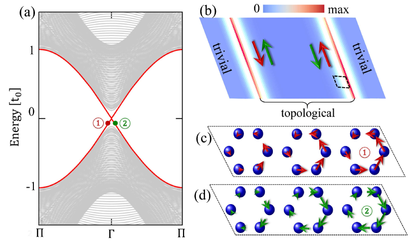
Figure 3: (Color online) (a) Band dispersion of a ribbon system of 36 hexagons with $t_{1}=1.1t_{0}$ cladded from both sides by 10 hexagons with $t_{1}=0.9t_{0}$. (b) Real-space distribution of the in-gap states associated with the red solid dispersion curves in (a). (c) and (d) Real-space distributions of current densities in pseudospin up and down channels at the momenta indicated by the red and green dots 1 and 2 in (a) within the rhombic area sketched by dashed line in (b); the excess currents in pseudospin up and down channels are indicated by red and green arrows in (b).

IV Topological edge states and associated conductances

IV.1 Topological edge states

In order to check the edge state in the present system, we consider a ribbon of hexagonal unit cells of $t_{1}=1.1t_{0}$ with its two edges cladded by hexagonal unit cells of $t_{1}=0.9t_{0}$. As can be seen in Fig. 3(a), additional states appear in the bulk gap as indicated by the red solid curves carrying double degeneracy. Plotting the spatial distribution of the corresponding wave functions, we find that the in-gap states are localized at the two interfaces between topological and trivial regions [see Fig. 3(b)]. As displayed in Fig. 3(c) [(d)], there is an excess upward (downward) edge current in the pseudospin-up (-down) channel associated with the state indicated by the red (green) dot in Fig. 3(a).

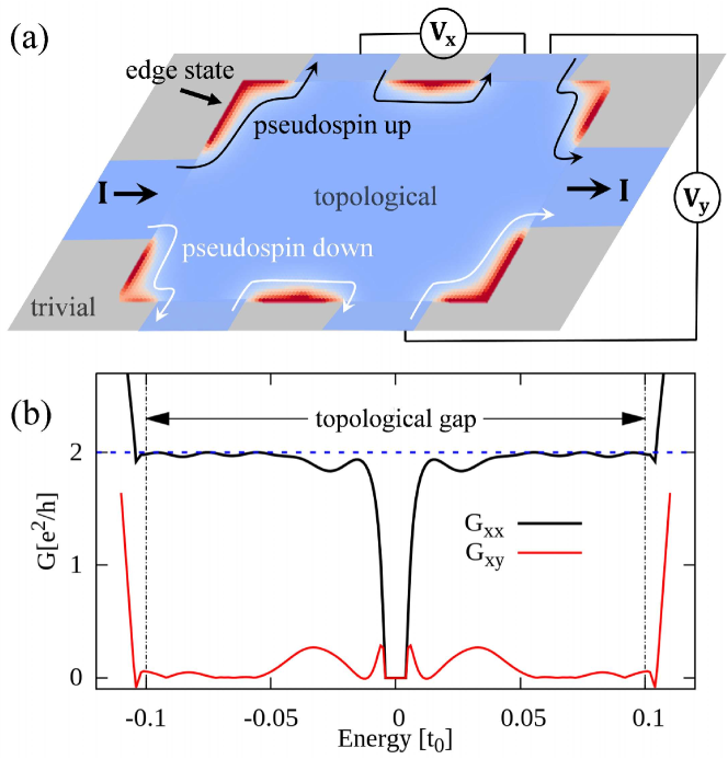
Figure 4: (Color online) (a) Schematic configuration of a six-terminal Hall bar where a topological sample (light blue region) with $t_{1}=1.1t_{0}$ is embedded in a trivial environment (gray region) with $t_{1}=0.9t_{0}$. The size of topological scattering region is $240a_{0}\times 120a_{0}$, and the width of each semi-infinite lead is $40a_{0}$. The injected current flows along the edges of topological sample as indicated by the red parts between electrodes. (b) Longitudinal and Hall conductances of the Hall bar as a function of energy of incident electrons. The on-site energy is taken $\varepsilon_{0}=0$. A rhombic topological sample is taken for ease of calculation.

IV.2 Hall and longitudinal conductances

At the interface between topological and trivial regimes, the crystal symmetry is reduced from $C_{6}$ to $C_{2}$, which breaks the pseudo-TR symmetry in contrast to the real TR symmetry. As the result, a mini gap of $\sim 0.01t_{0}$ [unnoticeable in the scale of Fig. 3(a)] opens in the otherwise gapless edge state at the $\Gamma$ point due to the coupling between two pseudospin channels. In order to quantitatively check possible backscatterings caused by this mini gap, we perform calculations on the longitudinal and Hall conductances based on a Hall bar system as sketched in Fig. 4(a). It is clear that the current $I$ injected from the left electrode divides itself into two branches according to the pseudospin states, namely pseudospin up (down) electrons can flow only in the upper (lower) edge of the Hall bar. By matching wave functions at the interfaces between the six semi-infinite electrodes and the topological scattering region AndoPRB1991 ; GrothNJP2014 , one can evaluate the transmissions of plane waves scattered among all the six leads, and then the longitudinal and Hall conductances, $G_{xx}=\rho_{xx}/(\rho_{xx}^{2}+\rho_{xy}^{2})$ and $G_{xy}=\rho_{xy}/(\rho_{xx}^{2}+\rho_{xy}^{2})$ respectively, by the Landauer-Büttiker formalism Landauer1999 , where $\rho_{xx}$ and $\rho_{xy}$ are the longitudinal and transverse resistances respectively. Similar to the case of QSHE with magnetic impurities TkachovPRL2010 , in the present system the values of conductivity deviate from the quantized ones when Fermi level falls in the mini gap of $\sim 0.01t_{0}$ as shown in Fig. 4(b). It is noticed, however, that both $G_{xx}$ and $G_{xy}$ heal quickly after several periods of oscillations that come from interferences between the two pseudospin channels. It is emphasized that almost perfectly quantized conductances $G_{xx}=2e^{2}/h$ and $G_{xy}=0$ Bernevig2006 ; Konig2007 are achieved for Fermi level beyond $0.04t_{0}$ up to the bulk gap edge at $0.1t_{0}$, where the edge states with almost perfect linear dispersions hardly feel the existence of the mini gap and essentially no appreciable backscattering exists.

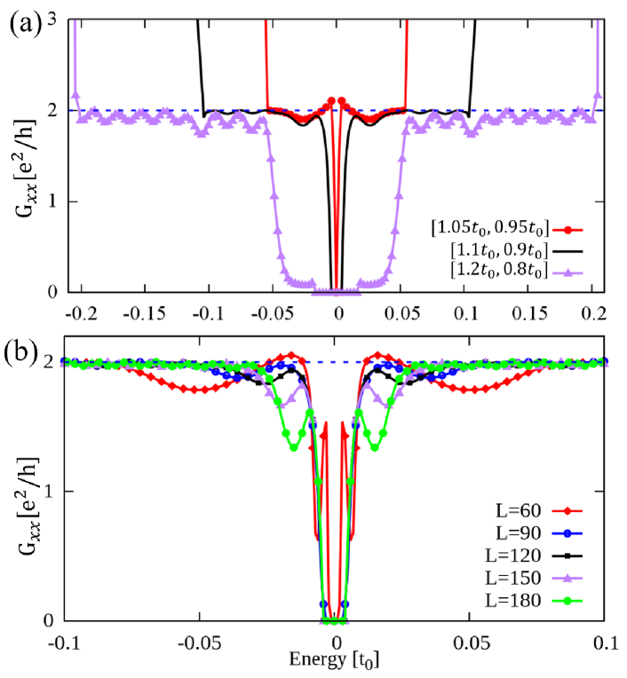
Figure 5: (Color online) Longitudinal conductance $G_{xx}$ of the topological sample given in Fig. 4(a) as a function of the energy of injected electrons: (a) for several typical values of inter-hexagon hopping integrals $[1.05t_{0},0.95t_{0}]$, $[1.1t_{0},0.9t_{0}]$ and $[1.2t_{0},0.8t_{0}]$, where the first (second) inside bracket is for the topological (trivial) region; (b) with several typical system sizes $2L\vec{a}_{1}\times L\vec{a}_{2}$, where the width of the electrodes is fixed at $40a_{0}$ and the inter-hexagon hopping integral is fixed at $t_{1}=1.1t_{0}$ and $t_{1}=0.9t_{0}$ for the topological and trivial regions respectively.

Now we discuss the hopping integral dependence of the longitudinal conductance. The size of scattering region is same as in Fig. 4(a) and fixed for all cases. As displayed in Fig. 5(a), $G_{xx}$ saturates to the quantized value $2e^{2}/h$ as expected for a $\mathbb{Z}_{2}$ topological state for all the cases with $t_{1}=1.05t_{0},1.1t_{0}$ and $1.2t_{0}$ in the topological region (whereas $0.95t_{0},0.9t_{0}$ and $0.8t_{0}$ in the trivial region correspondingly) when Fermi level is set away from the mini gaps, accompanied by oscillations due to interferences between two pseudospin channels.

Here we show the sample size dependence of the longitudinal conductance. We fix inter-hexagon hopping integrals at $1.1t_{0}$ and $0.9t_{0}$ in the topological and trivial regions respectively. As displayed in Fig. 5(b), $G_{xx}$ saturates in all cases to the quantized value $2e^{2}/h$ when Fermi level is shifted away from the mini gap. The topological edge transport remain unchanged when the topological sample becomes large.

V Real spin and QSHE

In addition to the pseudospin, the real spin degree of freedom also contributes to transport properties in realistic systems. In absence of the real SOC, the results presented in Fig. 4 remain exactly the same, with an additional double degeneracy due to the two real spin and thus $G_{xx}=4e^{2}/h$.

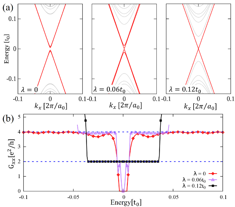
Figure 6: (Color online) (a) Dispersion relations and (b) longitudinal conductances of the topological system same as that given in Fig. 4(a) except that finite SOC is included.

An intrinsic SOC is induced when next-nearest-neighbor hoppings in honeycomb lattice are taken into account Kane2005a ; Kane2005b . The low-energy Hamiltonian around the $\Gamma$ point in Eq. (16) is then modified to

$$\tilde{H}(\mathbf{k})=\left(\begin{array}[]{cc}\tilde{H}_{+}(\mathbf{k})&\mathbf{0}\\ \mathbf{0}&\tilde{H}_{-}(\mathbf{k})\\ \end{array}\right)$$ (23)

with

$$\tilde{H}_{+}(\mathbf{k}) = \left(\begin{array}[]{cc}-\delta t-\nu\lambda+\frac{1}{2}a_{0}^{2}t_{1}\mathbf{k}^{2}&\frac{i}{2}a_{0}t_{1}k_{+}\\ -\frac{i}{2}a_{0}t_{1}k_{-}&\delta t+\nu\lambda-\frac{1}{2}a_{0}^{2}t_{1}\mathbf{k}^{2}\end{array}\right),$$ (26)

$$\tilde{H}_{-}(\mathbf{k}) = \left(\begin{array}[]{cc}-\delta t+\nu\lambda+\frac{1}{2}a_{0}^{2}t_{1}\mathbf{k}^{2}&\frac{i}{2}a_{0}t_{1}k_{-}\\ -\frac{i}{2}a_{0}t_{1}k_{+}&\delta t-\nu\lambda-\frac{1}{2}a_{0}^{2}t_{1}\mathbf{k}^{2}\end{array}\right),$$ (29)

where $\nu=1$ and $-1$ stand for real spin-up and -down states respectively. Therefore, for up real spin SOC enhances (suppresses) the topological gap in the pseudospin up (down) channel presuming $\lambda>0$ [see the left and central panels of Fig. 6(a)]. As far as $\lambda<\delta t$, the system remains the $\mathbb{Z}_{2}$ topological state associated with the pseudospin, where electrons with up pseudospin and down pseudospin counter propagate at edges, both carrying on up and down real spins. The longitudinal conductance $G_{xx}$ saturates to $4e^{2}/h$ as displayed in Fig. 6(b).

When SOC is increased to $\lambda=\delta t$, the pseudospin down (up) channel with real spin up (down) is driven into a semi-metallic state with zero band gap and the Dirac dispersion appears at the $\Gamma$ point. When SOC goes beyond $\delta t$, this Dirac dispersion opens a gap accompanied by a topological phase transition. The system now takes a QSHE state where at edges electrons with up real spin and pseudospin propagate oppositely to electrons with down real spin and pseudospin. Evaluating the longitudinal conductance, one finds that $G_{xx}$ is quantized exactly to $2e^{2}/h$ (see Fig. 6(b)), and as shown in the right panel of Fig. 6(a) there is no mini gap in the edge states, as protected by real time-reversal symmetry Kane2005a ; Kane2005b .

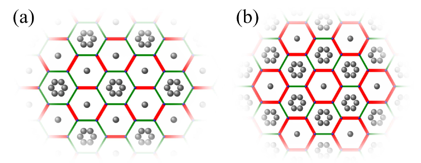
Figure 7: (Color online) Molecular graphene realized by decorating the Cu [111] surface with a triangular lattice of CO molecules: (a) $t_{1}>t_{0}$ generating topological state, (b) $t_{1}<t_{0}$ for trivial state. Gray balls are CO molecules decorated by STM techniques, and red thick bonds are shorter than green thin ones which generates the Kekulé hopping textures.

VI Discussions

Much effort has been devoted towards realizing the Dirac-like energy dispersion in artificial honeycomb lattices Polini2013 , ranging from optical lattices Tarruell2012 ; Wunsch2008 to 2D electron gases modulated by periodic potentials Gomes2012 ; GibertiniPRB2009 ; SGLouie2009 . All these systems provide promising platforms for realizing topological properties by detuning effective hopping energy among NN sites either by modulating muffin-tin potentials or bond lengthes periodically. To be specific, here we focus on how to achieve a topological state on the Cu [111] surface modulated by triangular gates of carbon monoxide (CO) molecules Gomes2012 . When extra CO molecules are placed at specific positions over the pristine molecular graphene, the bonds of the hexagons surrounding them are elongated since the CO clusters enhance local repulsive potentials and push electrons away from them, which reduces the corresponding electron hopping energies SGLouie2009 . It is extremely interesting from the present point of view that Kekulé hopping textures have already been achieved in experiments Gomes2012 . We propose to place extra CO atoms in the pattern displayed in Fig. 7(a), where the intra-hexagon hopping energy $t_{0}$ (green thin bonds) surrounding the CO clusters is reduced and the inter-hexagon hopping energy $t_{1}$ (red thick bonds) is enhanced relatively. According to the above discussions, the system displayed in Fig. 7(a) with $t_{1}>t_{0}$ should take a topological state. The Kekulé hopping texture in Fig. 7(b), dual to that shown in Fig. 7(a), was realized in experiments Gomes2012 , where the system takes a topologically trivial state because $t_{1}<t_{0}$.

The underlying idea of the present scheme for achieving the $\mathbb{Z}_{2}$ topological state is to create artificial orbitals carrying on opposite orbital angular momenta and parities with respect to spatial inversion symmetry, and to induce a band inversion between them by introducing a Kekulé hopping texture on honeycomb lattice. In the sense that it does not require SOC, the present state may be understood as a quantum orbital Hall effect. The topological properties can also be extended to photonic crystals Wu2015 , cold atoms, and even phonon systems where sound waves form band due to periodic configurations elastic materials.

VII Conclusion

We propose to derive topological properties by modulating electron hopping energy between nearest-neighbor sites of honeycomb lattice. Due to the Kekulé hopping texture with $C_{6}$ symmetry, atomic-like orbitals emerge, which carry a pseudospin degree of freedom characterizing a pseudo time-reversal symmetry and Kramers doubling. We reveal that the effective spin-orbit coupling associated with the pseudospin degree of freedom can be larger than the intrinsic one by orders of magnitude because of the pure electronic origin. The present work offers a new possibility for achieving topological properties and related novel quantum properties and functionalities at high temperatures.

- (1) P. R. Wallace, Phys. Rev. 71, 622 (1947).
- (2) K. S. Novoselov, A. K. Geim, S. V. Morozov, D. Jiang, Y. Zhang, S. V. Dubonos, I. V. Grigorieva, and A. A. Firsov, Science 306, 666 (2004).
- (3) M. I. Katsnelson, Graphene Carbon in Two dimensions (Cambridge University Press, 2012).
- (4) A. K. Geim, Science 324, 1530 (2009).
- (5) K. v. Klitzing, G. Dorda, and M. Pepper, Phys. Rev. Lett. 45, 494 (1980).
- (6) D. J. Thouless, M. Kohmoto, M. P. Nightingale, and M. d. Nijs, Phys. Rev. Lett. 49, 405 (1982).
- (7) F. D. M. Haldane, Phys. Rev. Lett. 61, 2015 (1988).
- (8) M. Z. Hasan and C. L. Kane, Rev. Mod. Phys. 82, 3045 (2010).
- (9) X.-L. Qi and S.-C. Zhang, Rev. Mod. Phys. 83, 1057 (2011).
- (10) C. L. Kane and E. J. Mele, Phys. Rev. Lett. 95, 226801 (2005).
- (11) C. L. Kane and E. J. Mele, Phys. Rev. Lett. 95, 146802 (2005).
- (12) F. Guinea, M. I. Katsnelson, and A. K. Geim, Nature Phys. 6, 30 (2010).
- (13) K. K. Gomes, W. Mar, W. Ko, F. Guinea, and H. C. Manoharan, Nature 483, 306 (2012).
- (14) B. Hunt et al., Science 340, 1427 (2013).
- (15) W. Yan, W.-Y. He, Z.-D. Chu, M. Liu, L. Meng, R.-F. Dou, Y. Zhang, Z. Liu, J.-C. Nie, and L. He, Nat. Commun. 4, 2159 (2013).
- (16) Z. Qiao, S. Yang, W. Feng, W.-K. Tse, J. Ding, Y. Yao, J. Wang, and Q. Niu, Phys. Rev. B 82, 161414 (2010).
- (17) Q.-F. Liang, L.-H. Wu, and X. Hu, New J. Phys. 15, 063031 (2013).
- (18) F. D. M. Haldane, and S. Raghu, Phys. Rev. Lett. 100, 013904 (2008).
- (19) L.-H. Wu, and X. Hu, Phys. Rev. Lett. 114, 223901 (2015).
- (20) L. Tarruell, D. Greif, T. Uehlinger, G. Jotzu, and T. Esslinger, Nature 483, 302 (2012).
- (21) L. Fu, Phys. Rev. Lett. 106, 106802 (2011).
- (22) T. H. Hsieh, H. Lin, J. Liu, W. Duan, A. Bansil, and L. Fu, Nat. Commun. 3, 982 (2012).
- (23) P. Dziawa et al., Nature Mater. 11, 1023 (2012).
- (24) S.-Y. Xu et al., Nat. Commun. 3, 1192 (2012).
- (25) J. J. Sakurai, Modern Quantum Mechanics (Addison Wesley, 1985).
- (26) A. H. Castro Neto, F. Guinea, N. M. R. Peres, K. S. Novoselov, and A. K. Geim, Rev. Mod. Phys. 81, 109 (2009).
- (27) B. A. Bernevig, T. L. Hughes, and S.-C. Zhang, Science 314, 1757 (2006).
- (28) L. Fu, and C. L. Kane, Phys. Rev. B 76, 045302 (2007).
- (29) T. Ando, Phys. Rev. B 44, 8017 (1991).
- (30) C. W. Groth, M. Wimmer, A. R. Akhmerov, and X. Waintal, New J. Phys. 16, 063065 (2014).
- (31) Y. Imry, and R. Landauer, Rev. Mod. Phys. 71, S306 (1999).
- (32) G. Tkachov, and E. M. Hankiewicz, Phys. Rev. Lett. 104, 166803 (2010).
- (33) M. König, S. Wiedmann, C. Brüne, A. Roth, H. Buhmann, L. W. Molenkamp, X.-L. Qi, and S.-C. Zhang, Science 318, 766 (2007).
- (34) M. Polini, F. Guinea, M. Lewenstein, H. C. Manoharan, and V. Pellegrini, Nature Nanotech. 8, 625 (2013).
- (35) B. Wunsch, F. Guinea, and F. Sols, New J. Phys. 10, 103027 (2008).
- (36) M. Gibertini, A. Singha, V. Pellegrini, and M. Polini, Phys. Rev. B 79, 241406 (2009).
- (37) C.-H. Park, and S. G. Louie, Nano Lett. 9, 1793 (2009).